Quadratic Curve Fitting-Based Image Edge Line Segment Detection: A Novel Methodology

Abstract

In the field of computer vision, edge line segment detection in images is widely used in tasks such as 3D reconstruction and simultaneous localization and mapping. Currently, there are many algorithms that primarily focus on detecting straight line segments in undistorted images, but they do not perform well in detecting edge line segments in distorted images. To address this quandary, the present study introduces a novel method of line segment identification founded on the principles of quadratic fitting. The method proposed utilizes the inherent property of a linear projection in a three-dimensional space, whereby it appears as a quadratic curve in a distorted two-dimensional image. This approach applies an iterative estimation process to ascertain the optimal parameters of the quadratic form that aligns with the edge contour. This process is facilitated by implementing an assumption and validation mechanism. Upon deriving the optimal model, it is then employed to identify the line segments that are encompassed within the edge contour. The experimental assessment of this novel method incorporates its application to both distorted and distortion-free image datasets. The method eliminates the necessity for preliminary processing to discarding distortions, thereby making it universally applicable to both distorted and non-distorted images. In addition to this, the experimental results based on the dataset indicate that the proposed algorithm in this paper achieves an average computational efficiency that is 27 times faster than traditional ones. Thus, this research will contribute to line segment detection in computer vision.

1. Introduction

Detecting line segments within images constitutes a significant challenge within the field of computer vision [1], and it has extensive ramifications across diverse applications such as camera calibration [2], pose estimation [3], image matching [4], image stitching [5], 3D object detection [6], and visual simultaneous localization and mapping (SLAM) [7].

Contemporary scholarly endeavors in the domain of edge line segment detection predominantly revolve around the identification of straight line segments within undistorted (or marginally distorted) images. Broadly, these techniques can be classified into the following categories: Hough transform [8], edge linking [9], and methodologies that are premised on gradient direction and magnitude [10]. The Hough transform technique translates image coordinates into a parameter space and identifies straight line segments through a process of accumulation voting, thereby delivering impressive accuracy and reliability. However, the technique necessitates parameter computation for each edge pixel within the image, leading to considerable computational load and compromising real-time efficiency. Furthermore, the Hough transform method relies solely on parameters to represent a line, rendering the precise localization of line segment endpoints challenging. In response to these shortcomings, Almazan et al. [11] implemented a perception grouping methodology based on the Hough transform technique to ascertain line segment endpoints and achieved commendable results. Conversely, edge linking methodologies extract initial line segments by pixel traversal, and are based on the substantial grayscale variations at image edges. The subsequent extension and merging of these initial segments are carried out using parameter fitting to yield reasonable and complete line segments. In comparison to the Hough transform method, edge linking techniques display superior noise resistance and computational efficiency. However, the quality of results obtained from edge linking methodologies heavily hinges on the reliability of the edge operator, potentially leading to a loss of some original image information. To counteract this issue, Dong et al. [12] introduced indicators of edge main direction and image gradient direction during the edge detection process, enhancing the line segment detection’s resistance to interference in edge linking methodologies. Lu et al. [13] proposed an adaptive parameter Canny operator to extract image edges, thereby enhancing the reliability of line segment detection in edge linking methodologies. Additionally, the gradient direction-based technique [14], unlike its counterparts, computes the gradient direction of pixels directly and groups pixels with similar gradients to establish regions for line segment detection. Yet, this method demands further refinement as it overlooks gradient magnitude information. Building upon the work of Burns et al. [14], Grompone et al. [10] proposed the classic line segment detector (LSD) method. This method considers both the gradient direction and the gradient magnitude of the image. By selecting pixels with extremum values of a gradient magnitude as seed points, it employs a region-growing approach to generate candidate line segment regions. Additionally, by combining hypothesis verification, it extracts the final line segments. The parameters of the LSD algorithm are adaptive, resulting in high accuracy and fast detection speed. Consequently, it has become a benchmark for modern line segment detection algorithms [15]. Extending the LSD algorithm, Salaun et al. [16] proposed a multiscale line segment detection algorithm, and Luo et al. [17] developed a line segment detection algorithm for high-resolution color images, delivering satisfactory results.

Based on the literature review presented above, it is evident that existing edge line segment detection methodologies are primarily designed for undistorted images. Hence, prior to employing these methodologies on distorted images, the pre-processing of these images would be required in addition to the standard denoising procedures [18]. This preliminary processing step not only amplifies the visual workload, especially for cameras with wide-angle lenses (such as fisheye lenses and spherical lenses), but also fails to effectively ensure the preservation of image information in wide-angle views. Consequently, detecting edge line segments and performing feature correction on the original distorted images presents a more effective approach for enhancing the speed of distortion correction, particularly for methods requiring high efficiency, such as the SLAM methods (e.g., ORB-SLAM [19] and VINS-MONO [20]). In response to these challenges, this paper presents a novel image edge line segment detection technique based on quadratic fitting, termed the QF-LSD method. Experimental outcomes demonstrate that, in comparison to mainstream line segment detection algorithms, the proposed method is capable of not only detecting edge lines in undistorted (or slightly distorted) images, but can also accurately and reliably identifying edge curve segments in highly distorted images. Additionally, the experiments demonstrate that the algorithm’s computational efficiency is 27 times faster than those in traditional approaches. The main contributions of this paper are as follows:

(1) This methodology leverages the property that a 3D straight line’s projection onto a distorted 2D image forms a quadratic curve. It iteratively estimates the quadratic curve model’s optimal parameters through hypothesis verification and uses this optimal model to find the longest and continuous pixel sequence as the edge line segment within the edge contour.

(2) To reliably extract the multiple edge line segments that potentially exist within the edge contour, each identified line segment within the contour is removed, and the remaining pixels in the contour form a new edge contour. The technique then re-estimates the quadratic curve model’s optimal parameters through hypothesis verification to extract new edge line segments, and this process is continued until no valid edge line segments can be extracted from the edge contour.

(3) Due to the edge detection method used in this article being independent of the camera’s distortion parameters, there is no need to preprocess the distorted images. This article conducts tests using image data from normal lenses, wide-angle lenses, and fisheye lenses, respectively.

The subsequent sections of this paper are structured as follows: Section 2 elucidates the mathematical derivations of the edge line segment model; Section 3 provides a detailed description of the edge line segment extraction algorithm based on quadratic fitting; Section 4 presents a performance comparison with the classical LSD algorithm using image data from normal lenses, wide-angle lenses, and fisheye lenses; and Section 5 concludes the paper.

2. Derivation and Parameter Solving of the Edge Line Segment Model

2.1. Construction of the Edge Line Segment Model

The straight edges in three-dimensional space possess collinearity during the imaging process, meaning that they remain straight when projected from a 3D space onto a two-dimensional image plane. Assuming the ideal equation of the projection of a 3D straight line edge onto a two-dimensional image plane is determined as follows:

$$a{x}_u+b{y}_u+c=0$$

(1)

where $(x_u,y_u)$ represents any arbitrary pixel point on the ideal projected straight line.

In the actual imaging process, camera lenses typically exhibit radial distortion, tangential distortion, and thin prism distortion due to manufacturing tolerances. However, the thin prism distortion and tangential distortion of the lens are typically negligible compared to radial distortion and can be ignored in practical applications. Therefore, the radial distortion of the camera lens can be represented using a single-parameter DM (division model) [21] as follows:

$$\left\{\begin{array}{c}{x}_u=\frac{x_d}{1+\lambda r_d^2}\hfill \\ y_u=\frac{y_d}{1+\lambda r_d^2}\hfill \end{array}\right.$$

(2)

where $(x_u,y_u)$ is the distortion-free image point, $(x_d,y_d)$ is the distortion image point corresponding to the distortion-free image, $\lambda$ is the distortion factor, and $r_d^2=x_d^2+y_d^2$. Bringing Equation (2) into Equation (1) we have the following:

$$a(\frac{x_d}{1+\lambda r_d^2})+b(\frac{y_d}{1+\lambda r_d^2})+c=0$$

(3)

Equation (3) is brought into $r_d^2=x_d^2+y_d^2$. After sorting, we have the following:

$$x_d^2+y_d^2+e{x}_d+f{y}_d+g=0$$

(4)

Among them, $e=\frac{a}{c\lambda }$, $f=\frac{b}{c\lambda }$, and $g=\frac{1}{\lambda }$. From (4), it can be seen that under the effect of lens distortion, the projection of a straight line segment in three-dimensional space in the two-dimensional plane is no longer an ideal straight line but a quadratic curve.

2.2. Solution of Edge Line Segment Model Parameters

From the derivation of Section 2.1, it is known that due to the distortion, each edge segment to be extracted in the actual image can be regarded as a quadratic curve, and the coefficients of the quadratic curve, i.e., the parameters of the image edge segment model, are calculated in this section.

Assuming that the extracted edge line segment consists of n pixel points, denoted as $\left\{\begin{array}{c}(x_{d,j},y_{d,j})|j=1,2,3,...,n\end{array}\right\}$, then it satisfies Equation (5):

$$x_{d,j}^2+y_{d,j}^2+e{x}_{d,j}+f{y}_{d,j}+g=0(j=1,2,3,...,n)$$

(5)

In order to obtain the exact coefficients e, f, and g of the quadratic curve, the error function is defined by (6):

$$F=\sum _n^{j=1}{(x_{d,j}^2+y_{d,j}^2+e{x}_{d,j}+f{y}_{d,j}+g)}^2$$

(6)

By solving the first-order partial derivative equation of Equation (6), i.e.,

$${\displaystyle \frac{\partial F}{\partial e}}=0;{\displaystyle \frac{\partial F}{\partial f}}=0;{\displaystyle \frac{\partial F}{\partial g}}=0$$

(7)

we can obtain the optimal solution of Equation (6). Then, by expanding and combining the like terms of Equation (7), we can have a matrix form as follows:

$$\begin{array}{cc}\hfill & \underset{A}{\underbrace{\left[\begin{array}{ccc}{\sum }_{j=1}^n{x}_{d,j}^2& {\sum }_{j=1}^n{x}_{d,j}{y}_{d,j}& {\sum }_{j=1}^n{x}_{d,j}\\ {\sum }_{j=1}^n{x}_{d,j}{y}_{d,j}& {\sum }_{j=1}^n{y}_{d,j}^2& {\sum }_{j=1}^n{y}_{d,j}\\ {\sum }_{j=1}^n{x}_{d,j}& {\sum }_{j=1}^n{y}_{d,j}& n\end{array}\right]}}\underset{X}{\underbrace{\left[\begin{array}{c}e\\ f\\ g\end{array}\right]}}=\hfill \\ \hfill & \underset{B}{\underbrace{\left[\begin{array}{c}-{\sum }_{j=1}^n(x_{d,j}^2+y_{d,j}^2)x_{d,j}\\ -{\sum }_{j=1}^n(x_{d,j}^2+y_{d,j}^2)y_{d,j}\\ -{\sum }_{j=1}^n(x_{d,j}^2+y_{d,j}^2)\end{array}\right]}}\Rightarrow AX=B\hfill \end{array}$$

(8)

The matrix containing the quadratic curve coefficients can be obtained by solving Equation (8) using the least squares method:

$$X={\left(A^{T}A\right)}^{-1}{A}^{T}B$$

(9)

3. Edge Line Segment Extraction Based on Quadratic Curve Fitting

From the derivation of the above mathematical equations, it is clear that each edge line segment to be extracted in the actual image should satisfy the quadratic curve model. The parameters of a quadratic curve model are calculated according to Equation (8) using at least three non-co-linear pixel points. Therefore, we can take the detected edge contour in the image, select three pixel points randomly from it, and estimate the optimal parameters of the quadratic curve model by continuously iterating. At the same time, this optimal model is used to find the continuous and longest image sequence in the edge contour, which is used as an edge segment of this contour. In addition, in order to avoid the problem that the edge contour contains multiple edge segments (as shown in Figure 1), which affects the reliability of subsequent detection, each edge segment extracted is removed from the edge contour, and the remaining pixel sequences constitute the new edge contour. Then, repeat the above steps of edge segment extraction until no more edge segments can be extracted from the edge contours. The above process is implemented as follows:

Step 1: The Canny operator [22] is used to detect the edge features in the input image, and the Moore-Neighbor algorithm [23] is used to find the edge contours. The edge contours whose length is smaller than ${\displaystyle \frac{1}{20}}$ of the image size are removed. Suppose M edge contours are extracted by the above steps (noted as the set $\left\{\begin{array}{c}{C}_i|i=1,2,3,...,M\end{array}\right\}$), where $C_i$ is any one edge contour.

Step 2: For the edge contour $C_i$, assume that it consists of n pixel points, and that it is denoted as $C_i=\left\{\begin{array}{c}(x_j,y_j)|j=1,2,3,...,n\end{array}\right\}$. From $C_i$, select three randomly non-co-linear pixel points $(x_1,y_1)$, $(x_2,y_2)$, and $(x_3,y_3)$ and bring them into Equation (9) to calculate the quadratic curve equation coefficients $e_k$, $f_k$, and $g_k$. Based on the current solution we obtain $e_k$, $f_k$, and $g_k$. Together with Equation (4), we define the error function as follows:

$$E=x_j^2+y_j^2+e_k{x}_j+f_k{y}_j+g_k$$

(10)

When the pixel points in $C_i$ satisfy Equation (10), then E’s value is smaller; otherwise, E’s value is larger. Therefore, by setting a threshold $\epsilon$ for the quadratic curve fitting error, it is possible to search for L from $C_i$ based on the magnitude of E, where L indicates the longest and continuous pixel sequence that satisfies Equation (10). In addition, this sequence can be recognized as an edge segment. The pseudocode for implementing the above process is illustrated by Algorithm 1:

Step 3: In Step 2, it is necessary to randomly select three non-collinear pixels from the edge contour set $C_i=\left\{\begin{array}{c}(x_j,y_j)|j=1,2,3,...,n\end{array}\right\}$. Therefore, pixel selection needs to be performed three times randomly. If there are a total of n pixels in the edge contour set $C_i$, and if the pixel length of one of the longest image sequences is denoted as L with a length of $len\left(L\right)$, then the probability that the selected pixels exactly fall on sequence L in a single random selection is (${\displaystyle \frac{len\left(L\right)}{n}}$). The probability that all three randomly selected pixels consecutively fall on sequence L is ${\left(\frac{len\left(L\right)}{n}\right)}^3$. The probability that none of the three sampled pixels fall on sequence L is

$$P=1-{\left(\frac{len\left(L\right)}{n}\right)}^3$$

(11)

In this algorithm, a threshold is set such that the probability of not selecting sequence L after K repeated samplings is less than 1%. If we want to obtain L in the set, it is necessary to repeat Step 2 K times, and the number of repetitions K is determined as follows:

$$P^K<0.01\Rightarrow K>ceil\left(\frac{lg0.01}{lgP}\right)$$

(12)

The function ceil(•) represents rounding up to the nearest integer. Therefore, as long as the number of iterations K is greater than the value in Equation (12), it is possible to reliably search for L in $C_i$. Furthermore, we define $D_i$ to store the continuous and longest edge segments. This means that the sequence L obtained from $C_i$ in Step 3 is added to the collection $D_i$ as an edge segment. After K iterations, if no L is found, $D_i$ remains empty, indicating that there are no satisfying edge segments in $C_i$.

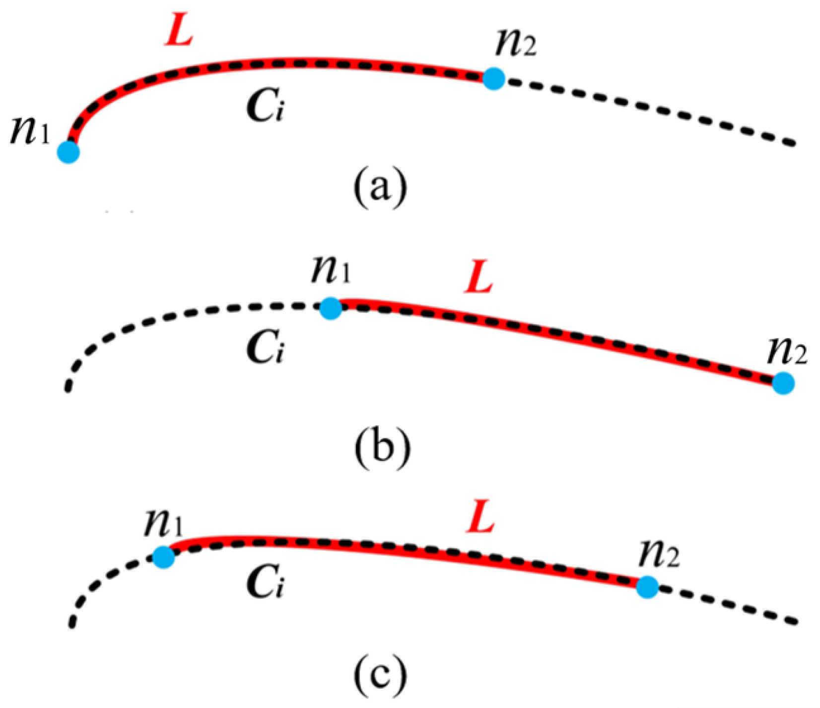
Step 4: After finding an edge line segment L in $C_i$, L is removed from $C_i$ and the remaining pixels form a new edge profile stored in R. Due to the three different distributions of L in the set $C_i$, deleting L corresponds to three different cases, as shown in Figure 2. The pseudocode for implementing the above process is illustrated by Algorithm 2:

As can be seen from Algorithm 2, the final R obtained either contains one edge contour, two edge contours, or is empty.

Step 5: Consider the edge contours in R as the new $C_i$, and repeat the steps from Step 2 to Step 4 until the contour set of R that can be formed by the remaining pixels is empty (which indicates that the edge segments in the initial $C_i$ that can satisfy the conditions in R are extracted).

Step 6: For the edge contours in the whole image $\left\{\begin{array}{c}{C}_i|i=1,2,3,...,M\end{array}\right\}$, Step 2 to Step 5 are repeated until the M contours are traversed to obtain the complete set of edge segments in the whole image $D=\left\{\begin{array}{c}{D}_i|i=1,2,3,...,M\end{array}\right\}$.

A complete representation of the algorithms in Step 1 to Step 6 above that use pseudocode are illustrated by Algorithm 3:

4. Experimental Analysis

The quadratic curve-based edge line segment detection algorithm (named the QR-LSD method) proposed in this paper is tested by real images and compared with the LSD straight line segment detection algorithm [10]. In order to make the algorithm more fair and reasonable in the experimental comparison, both the algorithm in this paper and the LSD algorithm are implemented in the same programming language. All codes were run on the same workstation with the following hardware configuration: i7-10700KF processor, 3.80 GHz main frequency, and 32 GB RAM.

The performance of the LSD algorithm and the proposed QF-LSD algorithm is depicted in Figure 3 and Figure 4a–x. The algorithms are tested on images from regular lenses (minor distortion), wide-angle lenses, and fisheye lenses to assess the edge line segment detection capabilities. Evidently, both the QF-LSD algorithm and the LSD algorithm can effectively and accurately extract edge line segments from images without distortion (or with minor distortion). However, the difference is that the LSD algorithm can detect more abundant edge detail information. From

Table 1. Evaluation metrics for line segment detection in undistorted images (unit: number of line segments).

Algorithm	Number of Line Segments									(a–h) Average Precision	(a–h) Average Recall
LSD method	Serial Number	a	b	c	d	e	f	g	h	0.465	0.381
	True Positive	67	133	130	194	190	161	569	154
	False Positive	74	139	154	230	201	183	620	223
	False Negative	109	207	223	329	295	268	887	257
QF-LSD method	Serial Number	a	b	c	d	e	f	g	h	0.878	0.218
	True Positive	49	103	80	115	103	70	123	105
	False Positive	13	10	13	11	6	14	12	17
	False Negative	127	237	273	408	382	359	1333	306

, we can see that its recall rate is high. This is because the LSD algorithm uses gradient direction and gradient magnitude information during the edge line segment detection process. On the other hand, the QF-LSD algorithm proposed in this paper is dependent on edge detection results; hence, the extracted edge segments are not as rich as those extracted by the LSD algorithm.

In images captured using wide-angle lenses (i–p) and fisheye lenses (q–x), the LSD algorithm can still detect richer edge details. Nevertheless, as the LSD algorithm is designed for straight line segment extraction in distortion-free images, it is incapable of accurately and completely describing edge arc segments in images with significant distortion. For example, in Figure 3q, the arc curve at the junction of the wall and ceiling extracted by LSD is formed by connecting multiple straight-line segments of different colors, whereas in Figure 4q the curve segment extracted by the QF-LSD algorithm is represented by a complete green curve segment. It can only approximate these segments using smaller straight line segments, thus leading to reduced accuracy in detection. To improve the LSD algorithm’s accuracy in aberrated images, a pre-correction of these images is necessary. This requires precise knowledge of the camera’s distortion parameters, which is often challenging for some online vision tasks. In contrast, the QF-LSD algorithm proposed in this paper is independent of the camera’s distortion parameters. It does not require a pre-processing of the distorted images. It can accurately and completely extract the edge arc segments in large distorted images. In vision tasks that typically rely on edge segments (e.g., visual pose measurement, visual SLAM, autonomous driving), the accuracy of the edge segment detection algorithm is more important than the amount that is detected. As long as accurate edge segments are extracted, the reliable implementation of corresponding vision tasks can be ensured. On the other hand, a low accuracy but high recall rate can only introduce more disturbing factors and larger errors in such vision tasks.

Table 2. Running time comparison (unit: seconds).

Algorithm	Serial Number									(a)–(x) Average Processing Time
LSD method	Regular lens images	a	b	c	d	e	f	g	h	18.90
		0.89	1.56	2.93	6.22	4.40	5.11	19.18	5.39
	Wide-angle lens image	i	j	k	l	m	n	o	p
		1.03	1.90	2.30	135.19	2.76	1.25	1.22	4.91
	Fisheye lens image	q	r	s	t	u	v	w	x
		1.25	26.14	64.19	157.43	2.07	0.78	2.86	2.78
QF-LSD method	Regular lens images	a	b	c	d	e	f	g	h	0.7
		0.39	0.49	0.70	0.81	0.72	0.69	0.94	0.82
	Wide-angle lens image	i	j	k	l	m	n	o	p
		0.36	0.41	0.65	1.28	0.57	0.32	0.55	0.68
	Fisheye lens image	q	r	s	t	u	v	w	x
		0.39	0.94	1.17	1.82	0.56	0.30	0.67	0.61

displays the time taken by both the LSD algorithm and the proposed QF-LSD algorithm to process each image. It can be observed that the operational efficiency of both algorithms is closely related to the image size and texture richness within the image. The larger the image size and the richer the texture information in the image, the longer both algorithms take to process the image. In comparison, the computational time of the QF-LSD algorithm presented in this paper is generally much smaller than that of the LSD algorithm.This is because the LSD algorithm not only calculates gradient direction and amplitude information when extracting straight line segments, but also employs region growth combined with hypothesis verification to obtain complete straight line segments, making the whole process more complex and time-consuming. Conversely, the QF-LSD algorithm proposed in this paper removes the edge segments from the contour after extraction, which improves the algorithm’s efficiency in identifying new edge segments within the remaining pixels. These measures effectively reduce the time cost of the QF-LSD algorithm.

In conclusion, compared to traditional straight line segment detection algorithms, the QF-LSD algorithm proposed in this paper is highly suitable for edge segment extraction from images with substantial distortion. It does not depend on the camera’s distortion parameters during edge detection, and it does not require a pre-processing of the distorted images. In addition, from the overall running time tested on the dataset, it is evident that the algorithm proposed in this paper achieves an average efficiency that is 27 times faster than traditional algorithms. Therefore, compared to traditional algorithms, it exhibits greater competitiveness and advantages in terms of real-time performance.

5. Conclusions

In this research, we introduced a method for image edge line segment detection that is founded on quadratic curve fitting. This approach capitalizes on the principle that a straight line in a three-dimensional space projects as a quadratic curve in a two-dimensional distorted image. The experiments demonstrate that, in addition to excellent detection accuracy, the method proposed in this paper is independent of camera distortion parameters and does not require a pre-correction of distorted images, thus exhibiting good practicality. Moreover, the algorithm’s computational efficiency is 27 times faster than those of the traditional approaches. We firmly believe that this algorithm will contribute to improving the real-time performance of vision-based autonomous driving technologies.