Amortized Bayesian Meta-Learning with Accelerated Gradient Descent Steps

Abstract

Recent meta-learning models often learn priors from observed tasks using a network optimized via stochastic gradient descent (SGD), which usually takes more training steps to convergence. In this paper, we propose an accelerated Bayesian meta-learning structure with a stochastic inference network (ABML-SIN). The proposed model aims to solve the training procedure of Bayesian meta-learning to improve the training speed and efficiency. Current approaches of meta-learning hardly converge within a few descent steps, owing to the small number of training samples. Therefore, we introduce an accelerated gradient descent learning network based on teacher–student architecture to learn the meta-latent variable ${\theta }_t$ for task t. With this amortized fast inference network, the meta-learner is able to learn the task-specific latent ${\theta }_t$ within a few training steps; thus, it improves the learning speed of the meta-learner. To refine the latent variables generated from the transductive amortization network of the meta-learner, SIN—followed by a conventional SGD-optimized network—is introduced as the student–teacher network to online-update the parameters. SIN extracts the local latent variables and accelerates the convergence of the meta-learning network. Our experiments on simulation data demonstrate that the proposed method provides generalization and scalability on unseen samples, and produces competitive/superior uncertainty estimations on few-shot learning tasks on two widely adopted 2D datasets with fewer training epochs compared to the state-of-the-art meta-learning approaches. Furthermore, the parameters generated by SIN act as perturbations on latent weights, enhancing the probability of accelerating the training efficiency of the meta-learner. Extensive qualitative experiments show that our method performs well across different meta-learning tasks in both simulated and real-world circumstances.

1. Introduction

The hallmark of human intelligence is the ability to learn quickly. For example, humans can recognize objects or make decisions quickly based on a few learning examples or minutes of experience. They can use learned skills to handle new cases that have never occurred before. We believe that our artificial agents should have the same capability to learn and adapt quickly from a few training examples, and should continue to learn as more data become available. This has generated vast interest in few-shot learning [1], which enhances data efficiency through shared information. The notion of “learning to learn” (or meta-learning) should be applied to train tasks and meet the computational requirements.

Meta-learning attempts to bestow machine learning models with the ability to train a meta-learner to perform well on a variety of training tasks [2]. For any unseen task, the meta-learner can learn to solve it efficiently by forming a task distribution similar to the one used for training. Though performances on few-shot learning have greatly increased in the past few years [3,4,5,6], it is still unclear how well these methods would perform in real-world tasks, where the evaluation tasks are different from the training dataset. Moreover, there is a lack of general-purpose tools for flexible and data-efficient learning [7], and there is still room for optimization in the meta-training process.

In addition to improving predictive accuracy for general tasks, it is also important for meta-models to provide good uncertainty predictions with a fast training process. Thus, we adopt the Bayesian method as a principled framework to provide uncertainty prediction. Approximate Bayesian methods are widely used to provide uncertainty prediction for deep learning models [8,9]. Bayesian meta-learning methods output a posterior distribution that correctly indicates the confidence level for unseen samples [2]. Researchers formulate the notion of the hierarchical Bayes (HB) model or empirical Bayes (EB) model, with the EB model restricting the learning of meta-parameters to point estimates. In our work, we consider EB model variational inference for meta-learning to simplify the training process without the HB formulation strength. This work focuses on the efficient usage of amortized variational inference for the Bayesian model with fast training steps. As such, we propose a synthetic inference network (SIN) combined with transduction for meta-learning, where the synthetic network produces the learned latent features over the neural network. During the training process, SIN refines the output of the transductive network that accelerates network convergence. We also propose a teacher–student network structure for the online training of SIN, where the conventional SGD-optimized network is treated as the teacher network. If not specified, we will denote the regular network optimized by SGD as the SGD network in the contents hereafter. The proposed method can converge a few steps after knowing the overall direction of the gradient descent. As illustrated in Figure 1, with collaborative training through the teacher–student network, the meta-training process is accelerated and the latent weights are optimized. Moreover, our method combines the generalization and scalability of the meta-learning model with uncertainty quantification, and it is robust to unseen datasets, owing to its posterior inference optimization. Our contributions are summarized as follows: (i) We propose a novel meta-learning model that utilizes a transductive amortization network to reduce the computational costs by optimizing the task-specific and global variables; (ii) the proposed synthetic inference network refines the output from the transductive network, significantly reducing the necessary training epochs compared with state-of-the-art methods; (iii) our method achieves quantitatively competitive performance on the Mini-ImageNet and Omniglot datasets, and superior visual performance on the ShapeNet dataset.

2. Related Work

The meta-learning literature usually interprets the meta-learning problem as Bayesian inference in a hierarchical graphical model, where ideas of HB or EB models for meta-learning have been widely used in the past few years. For example, Ref. [2] considered an HB model that improved MAML [5] to compute posteriors via amortized variational inference. Ref. [10] proposed a gradient-based algorithm, which minimized the objective function of meta-learning based on the HB model using the PAC-Bayesian Analysis. Ref. [11] introduced a new and rigorously formulated PAC-Bayes few-shot meta-learning algorithm, which implicitly learns a prior distribution of the model of interest. Ref. [12] used the EB model to construct a variational posterior by introducing a transduction network with a synthetic gradient. Other similar Bayesian VI-based HB methods are referred to [7,13,14]. Moreover, the empirical risk minimization (ERM) perspective has been successfully applied to a variety of few-shot learning models [15,16,17]. However, the HB model lacks the ability to handle large complex models or high-dimensional datasets due to its high computational costs for inference. Recent research developments have been used to scale Bayesian meta-learning into large datasets. For instance, Ref. [4] inferred episode-specific latent variables, and Ref. [10] learned the separated posterior weights for each task.

Other works focused on few-shot or one-shot learning-based Bayes methods proposed different perspectives. For instance, Ref. [18] proposed a Gaussian process, like the uncertainty neural process, which can be trainable by gradient descent. Ref. [2] proposed a method that efficiently amortizes hierarchical variational inference across tasks, learning a prior distribution over neural network weights so that a few steps of Bayes by Backprop will produce a good task-specific approximate posterior. Ref. [19] proposed a novel method that can adapt a pre-trained neural network to novel categories by directly predicting the parameters from the activations, which is regarded as amortized mean average precision (MAP) inference derived from the hyper-network [20]. Ref. [21] adapted the Bayesian decision theory to formulate the use of an amortization network for meta-learning so that it improves the state-of-the-art results.

Recent literature studies on PAC-Bayes meta-learning methods have focused on optimizing the generalization bounds for predictors with prior distributions. In [11], the authors extended previous bounds by optimizing the shared prior through the expectation–maximization (EM) algorithm. Rothfuss et al. [22] proposed a class of PAC optimal meta-learning algorithms with performance guarantees and a principled meta-level regularization by introducing Gaussian process priors with the SVGD [23] approximate optimization method. Other works [24,25] focused on improving generalization performance by introducing gradient augmentation or the regulation method at the inner level. Although these efforts strive to improve generalization performance, there are significant challenges in generalization on unseen tasks for meta-learning. Moreover, optimization of the meta-learning training procedure is also important and challenging as a means of improving training efficiency.

3. Meta-Learning with Amortized Bayesian Inference

As previously depicted, the goal of meta-learning is to train a model that suits a collection of tasks; such a meta-model works well on any task from this collection. Assume we are given T tasks for training, and the data are denoted as $\mathcal{D}=\{d^{\left(t\right)}:={(x^{\left(t\right)},y^{\left(t\right)}\}}_{t=1}^T$. Inputs are denoted as x and outputs as y. $\mathcal{D}$ can be elaborated as training data ${\mathcal{D}}_S^{\left(t\right)}={\left\{(x_n^{\left(t\right)},y_n^{\left(t\right)})\right\}}_{n=1}^{N_t}$ and test data ${\tilde{\mathcal{D}}}_Q^{\left(t\right)}={\left\{({\tilde{x}}_m^{\left(t\right)},{\tilde{y}}_n^{\left(t\right)})\right\}}_{m=1}^{M_t}$. According to [3], we denote the training samples as the support set and the test samples as the query set. For each task $i=1\cdots T$, ${\mathcal{D}}^{\left(i\right)}={\mathcal{D}}_S^{\left(i\right)}\bigcup {\tilde{\mathcal{D}}}_Q^{\left(i\right)}$. We revisit the classical hierarchical variational Bayes probabilistic model in this section, and propose using the amortized Bayesian meta-learning scheme by implementing a function of $x_t$ as the variational posterior.

3.1. Probabilistic Model

According to the classical hierarchical variational Bayes theory discussed in [10], the marginal likelihood of a hierarchical Bayes model is written in Equation (1) as follows:

$$p_f\left(\mathcal{D}\right)={\int }_{\theta }{p}_f\left(\mathcal{D}\right|\theta )p\left(\theta \right)={\mathit{\int }}_{\theta }\left[\prod _{t=1}^T{\mathit{\int }}_{\psi }{p}_f\left(d_t\right|{\psi }_t)p\left({\psi }_t\right|\theta )\right]p\left(\theta \right).$$

(1)

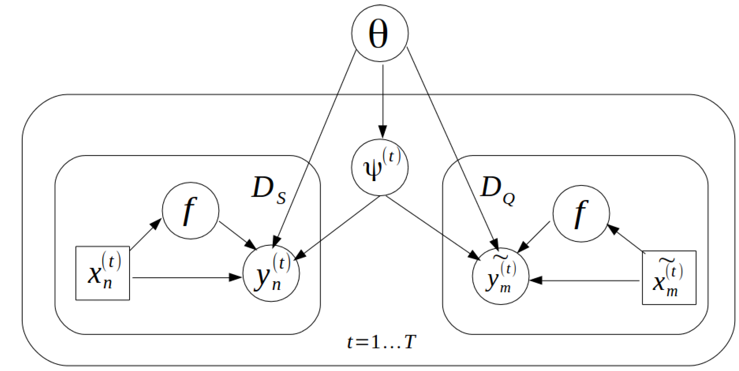
Its generative process is shown as a directed graphical model in Figure 2, where $\theta$ is denoted as the global latent variable. For each task t, a task-specific parameter ${\psi }_t$ is sampled from its priority $p\left({\psi }_t\right|\theta )$. Hierarchical variational inference can be used to estimate the lower bound of the likelihood in Equation (2) as follows:

$$\begin{array}{cc}\hfill & log{p}_f\left(\mathcal{D}\right)\hfill \\ \hfill & \ge {\mathbb{E}}_{q_{\theta }}\left[\sum _{t=1}^{T}log\left({\mathit{\int }}_{\psi }{p}_f\left(d_t\right|{\psi }_t)p\left({\psi }_t\right|\theta )\right)\right]-\mathrm{KL}\left(q\left(\theta \right)\right|\left|p\left(\theta \right)\right)\hfill \\ \hfill & \ge \sum _{t=1}^T\left[{\mathbb{E}}_{q_{{\theta }_t}}[log{p}_f\left(d_t\right|{\psi }_t)]-\mathrm{KL}(q_{{\theta }_t}\left({\psi }_t\right)\left|\right|p\left({\psi }_t\right|\theta ))\right]-\mathrm{KL}\left(q\left(\theta \right)\right|\left|p\left(\theta \right)\right),\hfill \end{array}$$

(2)

where $log{p}_f\left(\mathcal{D}\right)$ is denoted as the evidence lower bound (ELBO) on the log version. $q_{{\theta }_t}\left({\psi }_t\right)$ is the introduced variational distribution with parameter ${\theta }_t$. Given ${\theta }_t(0\le t\le T)$, variational inference solves the following optimization problem:

$$\begin{array}{cc}\hfill & \underset{\theta ,f,{\theta }_1,\cdots ,{\theta }_T}{argmin}{\mathbb{E}}_{q_{\theta }}\left[\sum _{t=1}^T-{\mathbb{E}}_{q_{{\theta }_t}}[log{p}_f\left(d_t\right|{\psi }_t)]+\mathrm{KL}(q_{{\theta }_t}\left({\psi }_t\right)\left|\right|p\left({\psi }_t\right|\theta ))\right]\hfill \\ & +\mathrm{KL}\left(q\right(\theta \left)\right|\left|p\right(\theta \left)\right)\hfill \\ \hfill & =\underset{\theta ,f,{\theta }_1,\cdots ,{\theta }_T}{argmin}\frac{1}{T}\sum _{t=1}^T\left[{\mathbb{E}}_{q_{{\theta }_t}}[-log{p}_f\left(d_t\right|{\psi }_t)]+\mathrm{KL}(q_{{\theta }_t}\left({\psi }_t\right)\left|\right|p\left({\psi }_t\right|\theta ))\right]\hfill \\ \hfill & +\mathrm{KL}\left(q\right(\theta \left)\right|\left|p\right(\theta \left)\right).\hfill \end{array}$$

(3)

Note that the optimization process in (3) results in heavy computational costs since it has to optimize T-different variational distributions $q_{{\theta }_t}(0\le t\le T)$ when T is large. To overcome this shortcoming, we introduce a transductive amortization network $\varphi$ that takes $x_n^{\left(t\right)}\in {\mathcal{D}}_S^{\left(t\right)}$ as input, and it outputs the variational distribution $q_{\varphi \left(d_t^S\right)}$. Here, we use $d_t^S$ to represent samples in ${\mathcal{D}}_S^{\left(t\right)}$ for short. The idea of amortized variational inference (AVI) was first introduced in [26] as a trainable autoencoder that produces variational parameters for each data point, and has been extended to Bayesian variational inferences [27]. Assume that $q_{\varphi \left(d_t^S\right)}$ follows the Dirac delta distribution (e.g., $q\left(\theta \right)=\mathbb{I}\{\theta ={\theta }^{*}\}$), where $\varphi \left(d_t^S\right)={\theta }_t^0$. For the k-th stochastic gradient descent iterate:

$${\theta }_t^{k+1}={\theta }_t^k+\eta {\nabla }_{{\theta }_t}\mathrm{KL}(q_{{\theta }_t^k}\left({\psi }_t\right)\left|\right|p_{f,\theta }\left({\psi }_t\right|d_t))\mathrm{with}{\theta }_t^0=\varphi ,$$

(4)

where $\eta$ denotes the descent step size. By conducting this optimization process up to the K-th step, such that ${\theta }_t^K={\varphi }^K\left(d_t^S\right)$, this guarantees that ${\theta }_t^K$ is a good approximation to its optimal value ${\theta }_t^{*}$. In summary, the optimization process contains the following two steps:

• initialize ${\theta }_t^0=\varphi \left(d_t^S\right)$
• for $k=0,\cdots ,K-1$, update ${\theta }_t^{k+1}$ via (4)

Let ${\ell }_t$ denote the loss function between the ground truth $y_t$ and the predicted value ${\hat{y}}_t$ for task t; we provide the gradient decomposition as follows:

$$\begin{array}{cc}\hfill & {\nabla }_{{\theta }_t}\mathrm{KL}(q_{{\theta }_t}\left|\right|p_{f,\theta })=\frac{1}{N}\sum _{i=1}^N\frac{\partial {\ell }_t(y_{t,i},{\hat{y}}_{t,i})}{\partial {\hat{y}}_{t,i}}\frac{{\hat{y}}_{t,i}}{\partial {\psi }_t}\frac{\partial {\psi }_t}{\partial {\theta }_t}\hfill \\ \hfill & +{\nabla }_{{\theta }_t}\mathrm{KL}(q_{{\theta }_t}\left|\right|p_{\theta }).\hfill \end{array}$$

(5)

Next, replacing each $q_{{\theta }_t}$ in (3), the optimization problem now becomes:

$$\begin{array}{cc}\hfill & \underset{\theta ,f,\varphi }{min}\frac{1}{T}\sum _{i=0}^T\left[{\mathbb{E}}_{q_{\varphi \left(d_t^S\right)}}[-log{p}_f\left(d_t\right|{\psi }_t)]+\mathrm{KL}(q_{\varphi \left(d_t^S\right)}\left({\psi }_t\right)\left|\right|p\left({\psi }_t\right|\theta ))\right]\hfill \\ \hfill & +\mathrm{KL}\left(q\right(\theta \left)\right|\left|p\right(\theta \left)\right).\hfill \end{array}$$

(6)

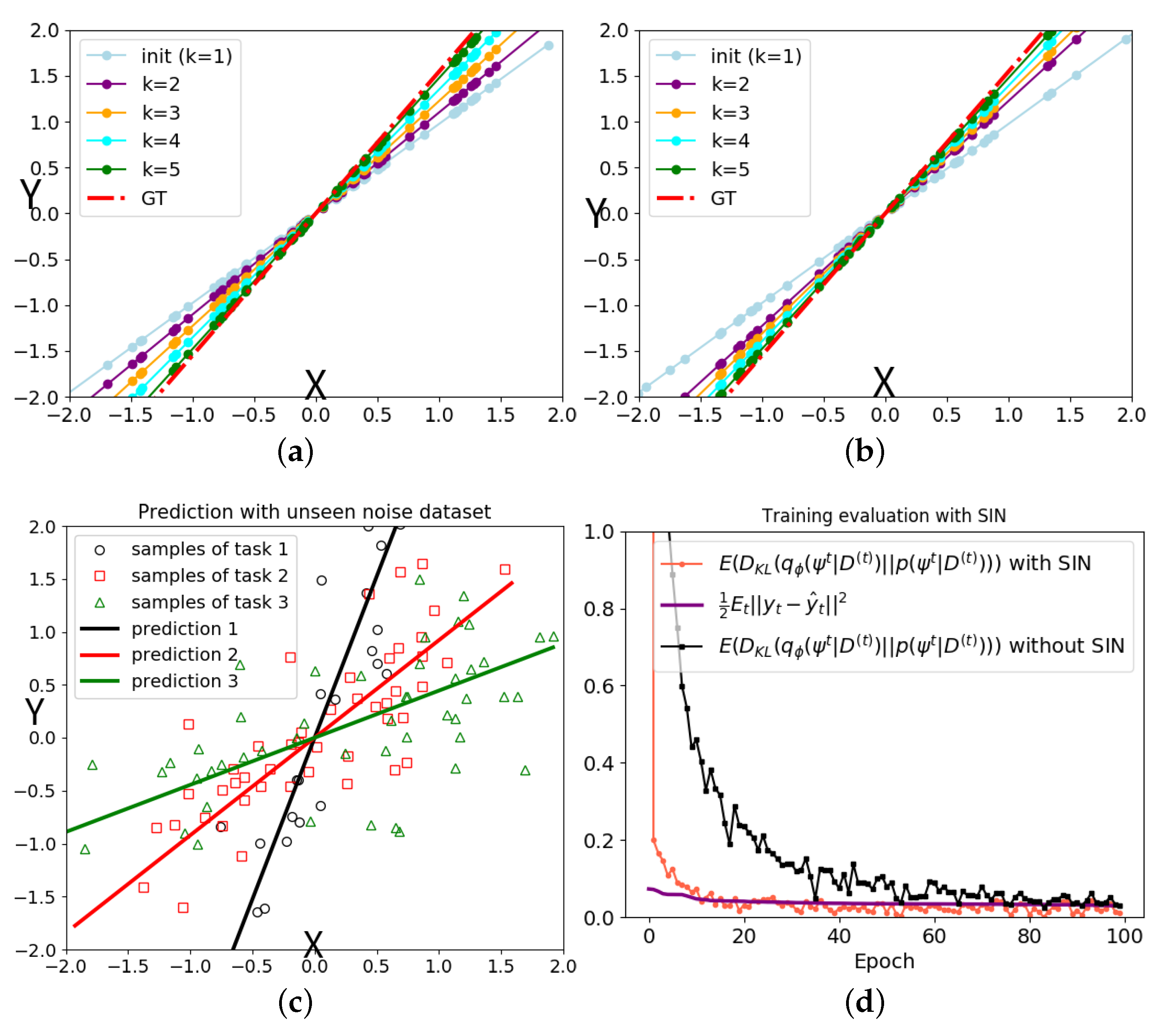
In conclusion, the meta-model is optimized with the feature network f and the hyperparameter $\theta$ from the Bayes formulation, together with the transductive amortization network $\varphi$.

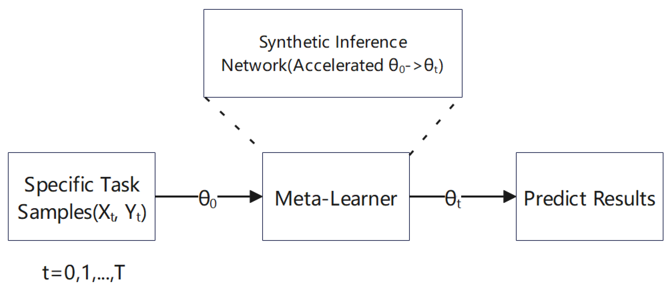
3.2. Fast Transductive Inference with the Synthetic Inference Network

We now introduce the proposed synthetic neural network for fast transductive inference. A side-by-side comparison between MAML and our method is displayed in Figure 3. In MAML, the global parameter $\theta$ is given an initialization according to its previous update, and it optimizes for a representation of $\theta$ that can quickly adapt to new tasks. In our method, we first introduce a transductive neural network $\varphi$ that outputs an initial distribution ${\theta }_t^0$ for different tasks t. Next, we propose a trainable synthetic inference network (SIN), which takes features of ${\theta }_t^0$ as the input and outputs its inferred parameters $\mathcal{I}$ for the refined variational distribution $q_{\varphi \left(d_t^S\right)}^{\prime }$. Then, the refined latent variable ${\theta }_t^{\prime }$ is formed by sampling from $\mathcal{I}$. With a few iteration steps, ${\theta }_t^{\prime }$ can reach ${\theta }_t^K$, converging to ${\theta }_t^{*}$.

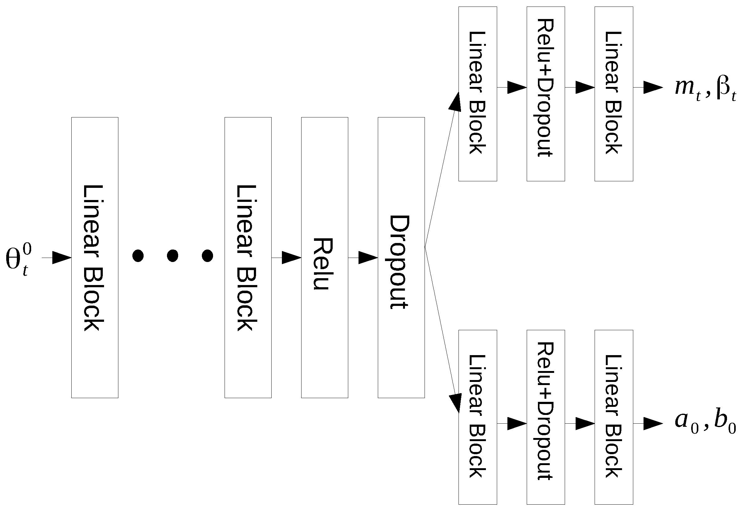
The details of SIN are given below. We let meta-parameter $\theta =\{{\mathbf{\mu }}_{\mathbf{\theta }},{\mathbf{\sigma }}_{\mathbf{\theta }}^{\mathbf{2}}\}$, where ${\mathbf{\mu }}_{\mathbf{\theta }}\in {\mathbb{R}}^D$, ${\mathbf{\sigma }}_{\mathbf{\theta }}^{\mathbf{2}}\in {\mathbb{R}}^D$ represent the mean and variance, respectively. For task-specific parameter ${\psi }_t$, its weight follows the normal distribution in Equation (7):

$$p\left({\psi }_t\right|\theta )=\mathcal{N}\left({\psi }_t|{\mathbf{\mu }}_{\mathbf{\theta }},{\mathbf{\sigma }}_{\mathbf{\theta }}^{\mathbf{2}}\mathbf{I}\right),$$

(7)

and the prior $p\left(\theta \right)$ is written in Equation (8):

$$p\left(\theta \right)=\mathrm{Dir}\left(\mathbf{\pi }\right|{\mathbf{\alpha }}_{\mathbf{0}})\prod _{t=1}^T\mathcal{N}\left({\mathbf{\mu }}_t\right|{\mathbf{m}}_0^{\left(t\right)},{\left({\beta }_0^{\left(t\right)}{\Lambda }_t\right)}^{-1})\mathrm{Wi}\left({\Lambda }_t\right|{\mathbf{L}}_0^{\left(t\right)},{\nu }_0^{\left(t\right)}),$$

(8)

where $\mathbf{\pi }=[{\pi }_1,\cdots ,{\pi }_t]$ follows the Dirichlet distribution with a symmetric prior ${\mathbf{\alpha }}_0={\alpha }_0\mathbf{I}$. ${\mathbf{m}}_0$, ${\beta }_0{\Lambda }_t$ denote the mean and precision matrix for the normal distribution, and ${\mathbf{L}}_0$ and ${\nu }_0$ represent the scale matrix and its freedom degree for the Wishart distribution. Note that when $dim\left({\theta }_t\right)=1\times N$, Wishart reduces to the Gamma distribution in Equation (9):

$$\mathrm{Wi}\left(\lambda \right|s^{-1},\nu )=\mathrm{Ga}\left(\lambda \right|\frac{\nu }{2},\frac{s}{2}).$$

(9)

Note that the exact posterior $p(\psi ,\theta |\mathcal{D})$ is a mixture of T distributions. We use the standard variational Bayes (VB) approximation to the posterior:

$$p(\theta ,{\mathit{\psi }}_{1:T}|\mathcal{D})\simeq q\left(\theta \right)\prod _{t=1}^{T}q\left({\psi }_t\right).$$

(10)

Meanwhile, it attempts to maximize the following lower bound:

$$\mathcal{L}=\sum _{\psi }\mathit{\int }q(\psi ,\theta )log\frac{p\left(f\right(x),\psi ,\theta )}{q(\psi ,\theta )}d\theta \le logp\left(\mathcal{D}\right)$$

(11)

For a detailed overview of the proposed meta-training with the SIN framework, we show a computational graph in Figure 1. A teacher–student network architecture is proposed for the fast convergence training of ${\theta }_t$. SIN is treated as an online trainable neural network with the stochastic gradient descent (SGD) network as its teacher network. Note that the learnable parameter of SIN is the inference parameter $\mathcal{I}$ for distribution $q_{\varphi \left(d_t^S\right)}^{\prime }$, where $\mathcal{I}=\{\mathit{m},\beta ,\mathbf{L},\nu \}$ denote parameters for the normal and Wishart distributions in (8). In fact, when ${\theta }_t^0\in {\mathbb{R}}^{1\times N}$, the Wishart distribution reduces to the Gamma distribution. Hence,

$$p\left(\theta \right)=\mathrm{Dir}\left(\mathbf{\pi }\right|{\mathbf{\alpha }}_{\mathbf{0}})\prod _{t=1}^T\mathcal{N}\left({\mu }_t\right|m_0^{\left(t\right)},{\left({\beta }_0^{\left(t\right)}{\tau }_t\right)}^{-1})\mathrm{Gamma}\left({\tau }_t\right|a_0,b_0),$$

(12)

where ${\beta }_0^{\left(t\right)}{\tau }_t=\frac{1}{{\sigma }_t^2}$ and $a_0$ and $b_0$ are the alpha and beta parameters for the gamma distribution. Note that $a_0=\frac{\nu }{2}$, $b_0=\frac{S}{2}$, where $S=1/N_t{\sum }_i{r}_{it}{(x_i-\overline{x})}^2$.

In our work, ${\theta }^0=\varphi \left(d^S\right)\in {\mathbb{R}}^{(T\times N)}$ represent T-way meta parameters as learnable initializations. The neural network $\varphi (·)$ takes the feature network output $f(x_n\in {\mathcal{D}}_S)$ as input, and $\varphi (·)$ is treated as the weight initialization network. Each task-specific parameter ${\theta }_t^0$ is passed through SIN to acquire $\mathcal{I}$. The proposed network structure is displayed in Figure 4 as a brief overview. It follows a multi-task learning structure, where the common network layers are denoted as the shared layers, while the last two separate layers output the two predicted groups of $\mathcal{I}$. Observe that SIN follows the online supervised learning scheme, where its training data ${\mathcal{D}}_{SIN}=\{{\theta }_t^0,\mathcal{M}\}$. In Figure 1, one can find that $\mathcal{M}$ is acquired through the variational Bayes inference with expectation maximization (VBEM). The EM method is introduced to maximize the lower bound of $\mathrm{KL}\left(q\left({\theta }^K\right)\right|\left|p\left({\theta }^K\right)\right)$, where ${\theta }^K$ is obtained from the SGD network with K-descent steps. As for the loss function, we use the simple MSE loss:

$$\begin{array}{cc}\hfill \mathcal{L}& =\gamma {\mathcal{L}}_0+(1-\gamma ){\mathcal{L}}_1,\hfill \end{array}$$

(13)

where ${\mathcal{L}}_0=\Vert {\hat{m}}_t-m_t{\Vert }_2+{\Vert {\hat{\beta }}_t-{\beta }_t\Vert }_2$ and ${\mathcal{L}}_1=\Vert {\hat{a}}_t-a_t{\Vert }_2+{\Vert {\hat{b}}_t-b_t\Vert }_2$. $\gamma$ is the weight factor whose value is set to $0.5$ as default.

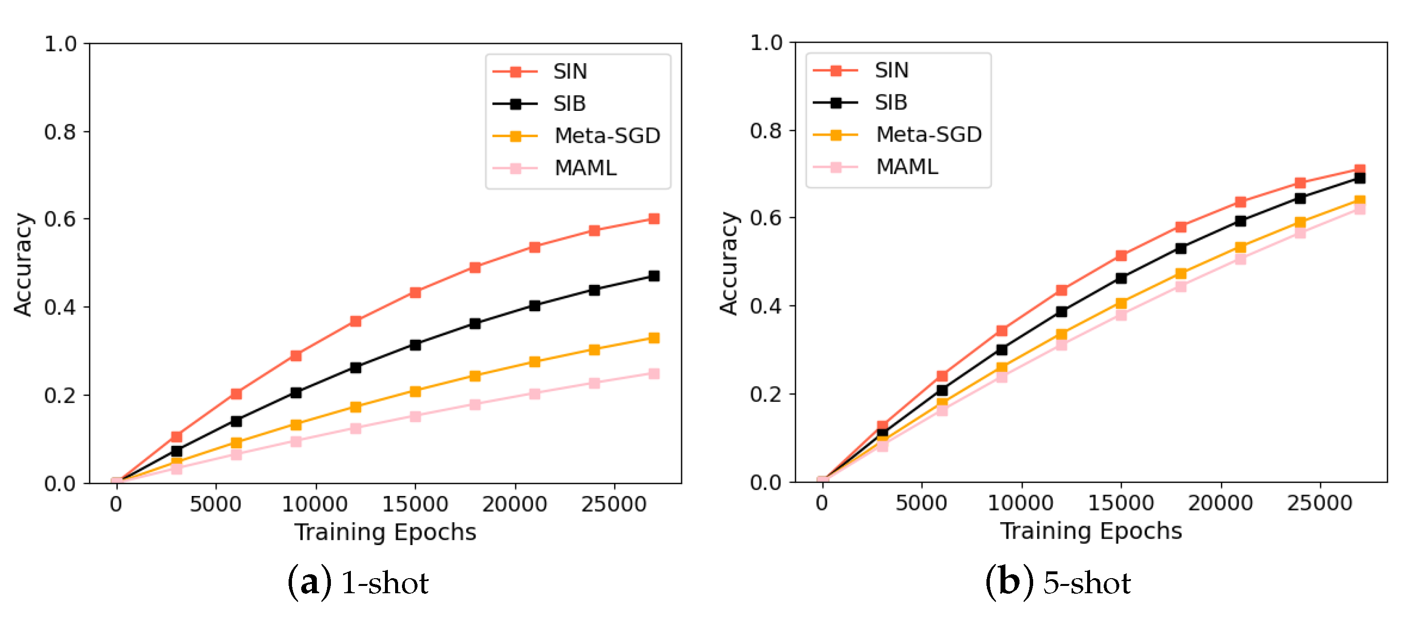
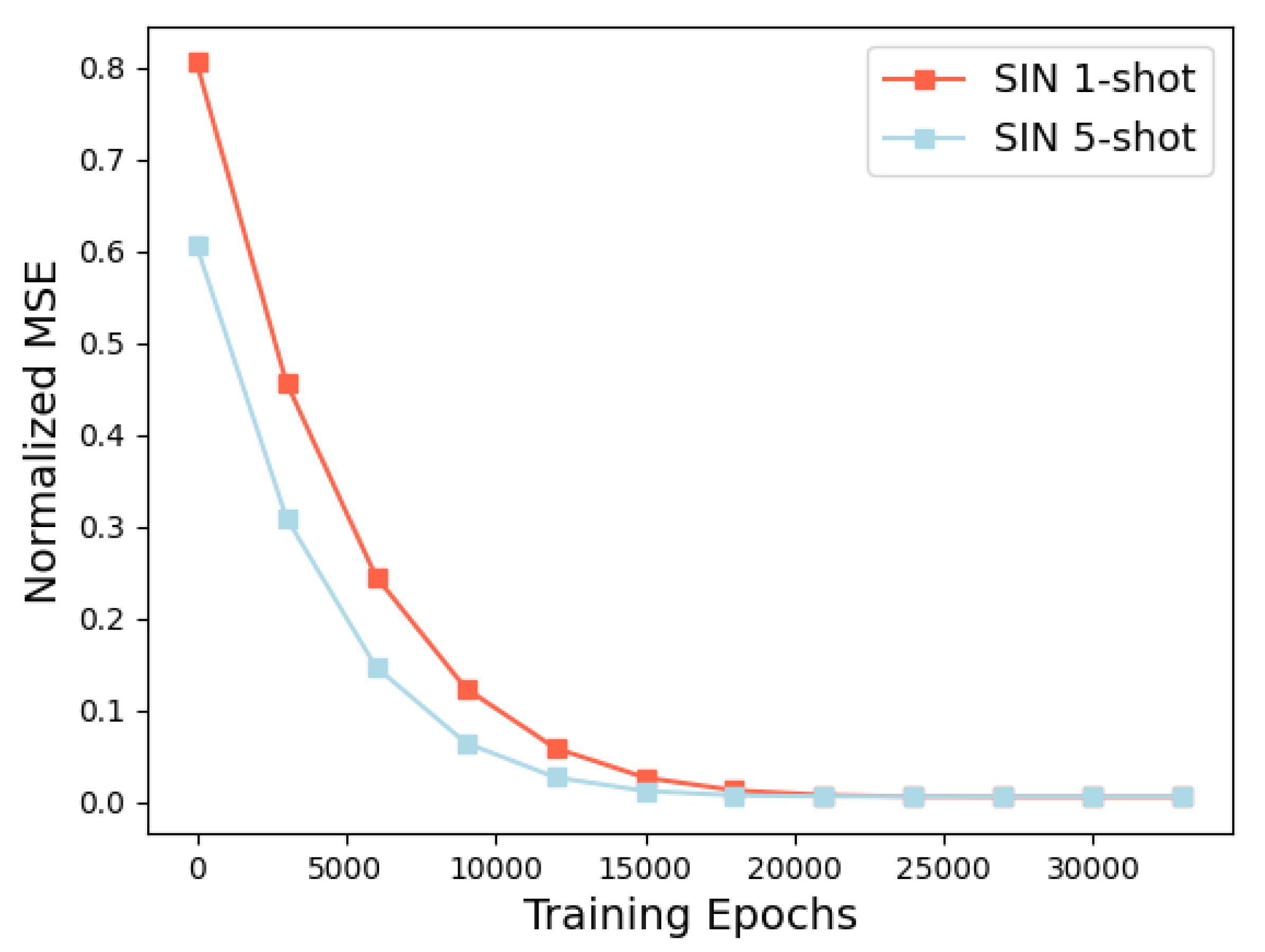
A detailed description of the proposed amortized Bayesian meta-training is depicted in Algorithm 1. The algorithm starts with the initializations of some meta-models, such as $\varphi \left(d^S\right)$, $\varphi \left(d^S\right)$, and f. For each task t, it computes ${\theta }_t^k$ via fast gradient descent steps, mixing SIN with the SGD network. It first uses the standard SGD network to obtain ${\theta }_t^k$. Meanwhile, the SGD network is used as a teacher network for training SIN. When the training process is valid, the output variable ${\theta }_t^{\prime }$ sampled from SIN can reach ${\theta }_t^{*}$ through fewer descent steps. After T training tasks are processed as the epoch, the transductive amortization network $\varphi$ is updated with the feature network f that has been fine-tuned. Notice that $\xi$ denotes an online training loss threshold, which indicates that the model can use the learned amortized network output ${\theta }_t^{\prime }$ for fast training. When the training process begins, SIN introduces a teacher–student network architecture for the prediction of ${\theta }_k$ (after k steps, the gradient descent of SGD). It uses a linear artificial neural network (ANN) to learn the specific latent parameters $\mathcal{I}$ related to ${\theta }_k$. The parameter set $\mathcal{I}=\{\mathit{m},\beta ,\mathbf{L},v\}$ represents parameters for normal and Wishart distributions in Equation (8). Note that we use these latent parameters to represent the posterior distribution of $q\left(\theta \right)$, which maximizes the following lower bound given in Equation (11). We first train both teacher and student networks in $K^{\prime }$ steps ($K^{\prime }\ll K$), after the student network learns the representation of the teacher network, then we use the inference of the student network directly to output $\mathcal{I}$. Note that $\mathcal{I}$ is obtained by the VBEM method of ${\theta }_t^k$. We generate the new ${\theta }_t’$ sampled from $\mathcal{I}$ and then assign it to ${\theta }_0$ for a middleware descent output. By applying a modest number of descent steps, where $K_0<<K$, the learned latent variable ${\theta }_t$ of the meta-learner can converge to the optimal point.

Algorithm  1 Amortized Bayesian meta-training with SIN.

Require:  the dataset $\mathcal{D}$; learning rate $\eta$; iteration number K;    number of tasks T. 1:  Initialize meta-model $\theta =\{{\mathbf{\mu }}_{\theta },{{\mathbf{\sigma }}_{\mathbf{\theta }}}^2\}$, $p\left(\theta \right)\sim$ (8). 2:  Initialize the transductive amortization network $\varphi \left(d^S\right)$ and the pre-trained feature network f. 3:  Initialize loss function ${\mathcal{L}}^{\left(t\right)}=inf$ for T tasks of SIN. 4:  while not converged do 5:     for  t = 1 to T do 6:         Sample a task t’s data ${\mathrm{x}}^t$ with its related support set ${\mathcal{D}}_S^{\left(t\right)}$ and query set ${\hat{\mathcal{D}}}_Q^{\left(t\right)}$. 7:         Compute ${\theta }_0^t=\varphi \left(f\left({\mathbf{x}}^t\right)\right)$, where $x^t\in {\mathcal{D}}_S^{\left(t\right)}$. 8:       if  ${\overline{\mathcal{L}}}^{\left(t\right)}<\xi$ then 9:           Compute ${\theta }_t^{\prime }$ sampled from the output $\hat{\mathcal{I}}$ of SIN, assign ${\theta }_t^0={\theta }_t^{\prime }$ sampled from $\hat{\mathcal{I}}$. 10:         for  $k=1,\cdots ,K^{\prime }(K^{\prime }\ll K)$ do 11:             Compute ${\theta }_t^k$ via (4) with learning rate $\eta$ 12:         end for 13:       else 14:         for $k=1,\cdots ,K$ do 15:           Compute ${\theta }_t^k$ via (4) with learning rate $\eta$ 16:         end for 17:       end if 18:       Implement the VBEM method for ${\theta }_t^k$ to compute the inferred parameter ${\mathcal{I}}^{\left(t\right)}$. 19:       Update $\mathrm{w}\leftarrow \mathrm{w}-\eta {\nabla }_{\mathrm{w}}\mathcal{L}\left({\mathcal{I}}^{\left(t\right)}\right)$ with $K_0$ ($K_0<K$) iterations, where $\mathit{w}$ denotes the weight of SIN. 20:     end for 21:     Update $\mathit{\varphi }\leftarrow \mathit{\varphi }-{\eta }_{\mathit{\varphi }}\mathrm{KL}(q_{\varphi \left(d^S\right)}\left(\psi \right)\left|\right|p\left(\psi \right|\theta ))$. 22:     Optionally, fine-tune $f\leftarrow f+\eta {\nabla }_{f}log{p}_f\left(d_t\right|{\psi }_t)$. 23: end while

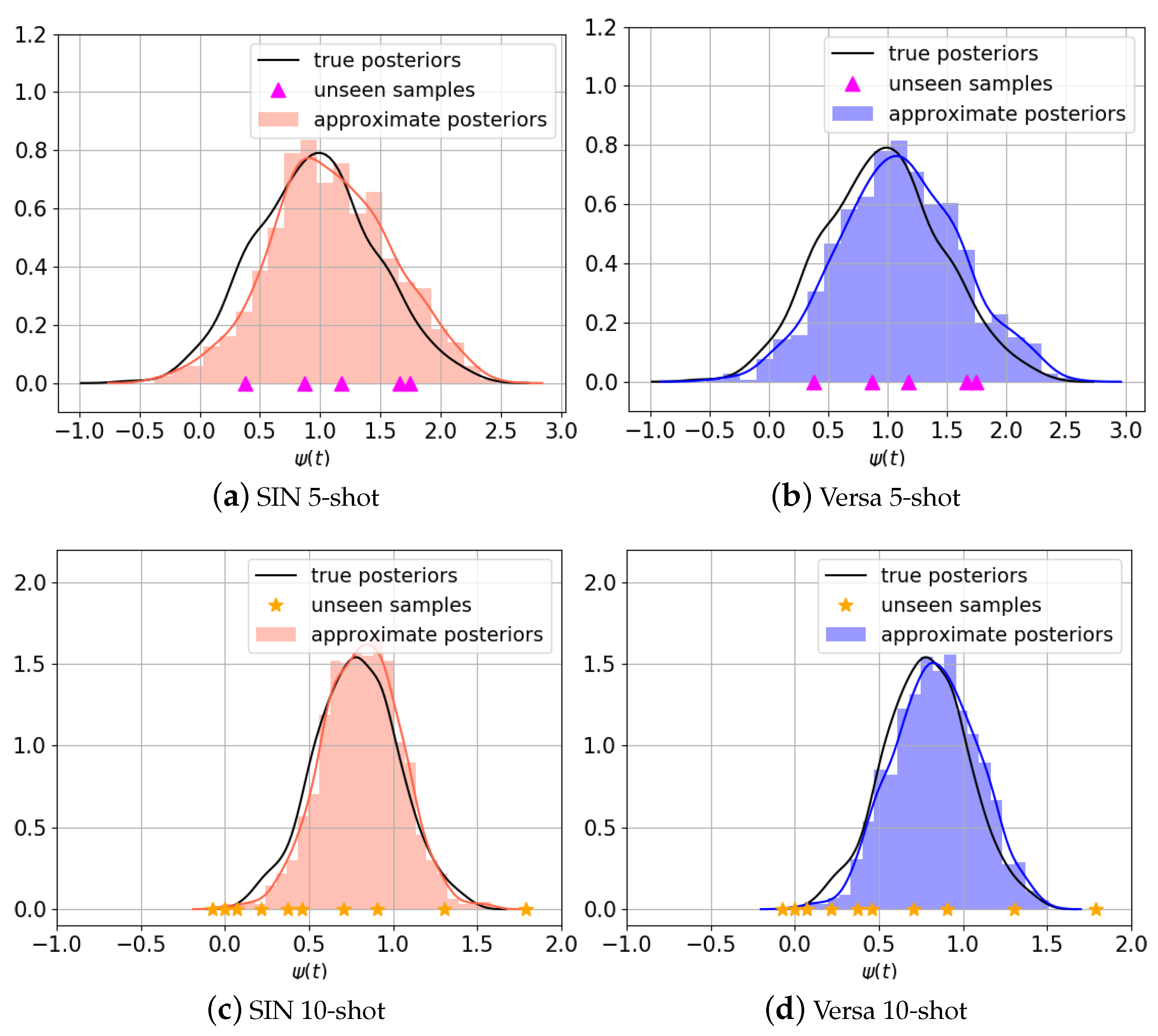
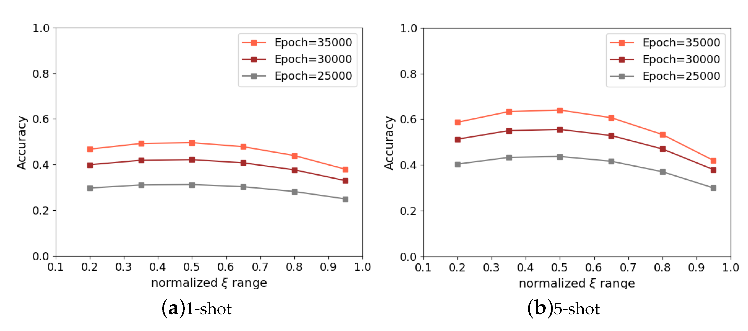
To summarize the architecture of the proposed ABML-SIN model, we provide a clear learning structure of our model, depicted in Figure 5. We can see that the architecture of ABML-SIN is embedded into the meta-learner module. It helps the meta-learner to quickly infer the learned latent posterior ${\theta }_t$ for task t based on the prior ${\theta }_0$. ABML-SIN provides an amortized synthetic inference network (ASIN) to use the pre-trained student network for fast ${\theta }_t$ output. For different task numbers $t=0,\cdots ,T$, the inference network outputs different posterior values ${\theta }_t$ related to the prediction results.

4. Experiments

To evaluate the proposed amortized Bayesian SIN meta-learning model on several few-shot learning tasks, we begin with simulation experiments for posterior inference to investigate the performance of the proposed amortized inference network (SIN). We then test few-shot classification results based on Omniglot and Mini-ImageNet datasets. Also, the performance of our method is analyzed based on accuracy, inference speed, and convergence time, varying in ways and shots, compared with other state-of-the-art meta-learning methods.

4.1. Data Posterior Inference Examples

We begin the posterior inference example with emulated data generated from a Gaussian distribution whose mean value is different from the task in Equation (14):

$$\left\{\begin{array}{cc}\hfill & p\left({\psi }^{\left(t\right)}\right|\theta )=\mathcal{N}({\psi }^{\left(t\right)};\mu ,{\sigma }^2)\hfill \\ \hfill & p\left(x_n^{\left(t\right)}\right|{\psi }^{\left(t\right)})=\mathcal{N}(x_n^{\left(t\right)};{\psi }^{\left(t\right)},{\sigma }_x^2),\hfill \end{array}\right.$$

(14)

where $p\left(\theta \right)$ follows the delta distribution $\delta \left(\theta \right)$. According to Gordon et al. [7], we set the sample number $N\in \{5,10\}$ for the support set and $N^{\prime }=15$ for the query set. The transductive amortized neural network $\varphi$ is defined as follows:

$$\left\{\begin{array}{cc}\hfill & {\mu }^{\left(t\right)}=\sum _{n=1}^N{x}_n^{\left(t\right)}{\omega }_{\mu }^n+b_{\mu }\hfill \\ \hfill & log{\sigma }^{\left(t\right)}=\sum _{n=1}^N{x}_n^{\left(t\right)}{\omega }_{\sigma }^n+b_{\sigma },\hfill \end{array}\right.$$

(15)

where parameter sets ${\theta }^0=\{{\mathbf{\omega }}_{\mathbf{\mu }},{\mathbf{\omega }}_{\mathbf{\sigma }},b_{\mu },b_{\sigma }\}$ are trained parameters for $\varphi$, and $q_{\varphi }\left(\psi \right|D^{\left(t\right)})=\mathcal{N}(\psi ;{\mu }^{\left(t\right)},{\sigma }^{\left(t\right)2})$. In this case, since the dimensions of these trainable parameters are low, it is unnecessary to use VI to inference the refined parameters $\mathcal{I}$ in SIN. Instead, we use a simple encoder–decoder network that takes ${\theta }^0$ as the input and outputs ${\theta }_t^{\prime }$ directly since few parameters with low dimensions are easy to converge. The objective log-likelihood function for optimization is given in Equation (16):

$$\mathcal{L}(\theta ,\varphi )=\frac{1}{T}\sum _{T}log\frac{1}{N}\sum _{n=1}^{N}p\left(x_n^{\left(t\right)}\right|{\psi }^{\left(t\right)},\theta ),{\psi }^{\left(t\right)}\sim q_{\varphi }\left(\psi \right|{\mathcal{D}}^{\left(t\right)},\theta )$$

(16)

For implementation details, we generate $T=250$ tasks with 5 shots and 10 shots for training observations. The teacher network (SGD) and the student network (SIN) are both trained to convergence by using the Adam [28] optimizer, and the generated data samples are rearranged as mini-batches of tasks for training input. To generate this dataset, we use N random variables for $\mu$ and $\sigma$ to generate the support set (small training samples) and query set (unseen samples of $\mu$ and $\sigma$). After the loss function is converged, $q_{\varphi }\left(\psi \right|\mathcal{D})$ is inferred by SIN with the learned amortization parameters. Figure 6 shows the approximate posterior distributions inferred from unseen test samples and the true posteriors for two-shot cases. We compare the output of SIN with Versa [7], where Versa uses an end-to-end stochastic training that optimizes the likelihood function corresponding with $\varphi$ and $\theta$. We can see that SIN can output the approximate posterior that closely resembles its true posterior, and its inference results are close to the standard amortization network.

Another simulation example is made for spinning-line regression of zero-shot learning. Denote $\mathcal{D}={\left\{(x_n,y_n)\right\}}_{n=1}^N$, the output for $x_n$ is $y_n=w·x_n$. Similar to the previous example, we set ${\theta }^0=\{\mathbf{\omega },b\}$ and $q_{\varphi }\left(\psi \right|D^{\left(t\right)})=\mathcal{N}(\psi ;{\mu }_{\psi }^{\left(t\right)},{\sigma }_{\psi }^{\left(t\right)2})$. Specifically, we have ${\mu }_{\psi }^{\left(t\right)}={\sum }_n{x}_n^{\left(t\right)}{\omega }_n+b$. To generate the dataset, we first sample i.i.d. Gaussian random variables $x_n\sim \mathcal{N}(\mu ,\sigma )$. Next, we sample slope $w=\frac{1}{N}{\sum }_n{x}_n+\mathcal{N}({\mu }_w,{\sigma }_w^2)$ from $p\left(\psi \right|\mathcal{D})$. The posterior distribution $p\left(\psi \right|\mathcal{D})\sim \mathcal{N}(\overline{x_n}+{\mu }_{\psi },{\sigma }_{\psi }^2)$, and the log-likelihood function is defined in Equation (17):

$$\mathcal{L}(\theta ,\varphi )=\frac{1}{T}\sum _{T}log\frac{1}{N}\sum _{n=1}^{N}p\left(y_n^{\left(t\right)}\right|x_n^{\left(t\right)},{\psi }^{\left(t\right)},\theta ),$$

(17)

where ${\psi }^{\left(t\right)}\sim q_{\varphi }\left(\psi \right|{\mathcal{D}}^{\left(t\right)},\theta )$. In this example, we initialize $n=32,\mu =0,\sigma =1,{\mu }_w=1,$${\sigma }_w=0.1$. The number of tasks T is set to 240 for both the train and test sets, and the learning rate is given as 0.001 with the mini-batch size of 8. We also use a simple encoder–decoder network for SIN, which takes ${\theta }_t^0$ as the input and outputs ${\theta }_t^{\prime }$. Figure 7 shows some experimental results for spinning-line zero-shot learning. We trained our model over 100 epochs by using the ADAM optimizer. From Figure 7a,b, we see that ${\theta }_t^k(k=\{1\cdots 4\})$ steps gradually toward the ground truth. Also, when SIN converges, it outputs an appropriate value ${\theta }_t^{\prime }$, which is close to ${\theta }^{*}$, and only a few iteration steps can make ${\theta }_t^k$ close to the ground truth.

Figure 7c shows the performance of SIN for the unseen test dataset with extra noise points. In this case, we set $x_n\sim \mathcal{N}(\mu ,\sigma )+\epsilon$, where $\epsilon \sim \mathcal{N}(0,{\sigma }_{\epsilon })$ denotes Gaussian white noise. The test data are generated from $x_n$ with noise components. We find that the proposed method can predict the regression line clearly given the unseen samples under the task of zero-shot learning. Figure 7d displays the value of the loss function and KL divergence of $q_{\varphi }\left(\psi \right|\mathcal{D})$ and $p\left(\psi \right|\mathcal{D})$ during the training process, which indicates that SIN is able to accelerate the training convergence process and identify the descent direction after meta-learning.

We provide another simulation example of posterior latent inference based on the MNIST dataset. In this case, dataset $\mathcal{D}={\{{\mathbf{x}}_n,y_n\}}_{n=1}^N$, where ${\mathbf{x}}_n$ denotes the image’s gray pixels and $y_n$ denotes its label. The latent variable $\mathbf{z}\in {\mathbb{R}}^{1\times 2}$ has two-dimensional values. We aim to find the implicit distribution for z, where $z\sim q_{\varphi }\left(\psi \right|\mathcal{D},\theta )$, which one can sample from, but the density cannot be evaluated. We set the prior distribution $p\left(z\right)\sim \mathcal{N}(0,{\sigma }^{\left(t\right)2})$, and its unnormalized posterior follows:

$$p\left(z\right|\mathcal{D})\propto log(\mathcal{Q})-T(\mathrm{x},y)/\mathcal{Q}$$

(18)

where $\mathcal{Q}={\beta }_0+{\beta }_1(\mathrm{ReLu}{\left(x_1\right)}^3+\mathrm{ReLu}{\left(x_2\right)}^3)$ denotes the exponential random variable with parameter $\beta$, $T(\mathrm{x},y)\Rightarrow \mathcal{D}\to \mathbb{R}$ is the mapping function that maps $\{\mathrm{x},y\}$ into a real value. We rearrange the KL divergence of $p\left(z\right|\mathcal{D})$ and $q_{\varphi }\left(z\right|\mathcal{D})$ in a discrete form:

$$\begin{array}{cc}\hfill & \frac{1}{N}\sum _{n=1}^N\mathrm{KL}[q_{\varphi }\left(z\right|\mathcal{D})\left|\right|p\left(z\right|\mathcal{D})]=\frac{1}{N}\sum _{n=1}^N\mathrm{KL}[q_{\varphi }\left(z\right|\mathcal{D})\left|\right|p\left(z\right)]-\hfill \\ \hfill & \frac{1}{N}\sum _{n=1}^N{\mathbb{E}}_{z\sim q_{\varphi }\left(z\right|\mathcal{D})}logp\left(\mathcal{D}\right|z)+p\left(\mathcal{D}\right).\hfill \end{array}$$

(19)

In this sub-experiment, the training samples are collected from the MNIST dataset and manually create $T(\mathrm{x},y)$, which maps 0–9 into a monotone nonlinear set $\mathbb{T}$. We let $\mathbb{T}=\{-10,0,4,8,12,\cdots ,150\}$, and generate the ground-truth posterior of z from $p\left(\psi \right|\mathcal{D},\theta )$. As shown in Figure 8, the samples from the MNIST dataset correspond to the posterior distribution $p\left(z\right|\mathcal{D})$ one by one. We use the pre-trained CNN network for the MNIST feature network by removing the last sigmoid layer. Hence, ${\theta }_t^0=\varphi \left(d_t^S\right)\in {\mathbb{R}}^{(T\times N)}$, whereas $T=10$ and $N=1024$. The network structure of SIN is given in Figure 4, where four linear dense layers are used followed by a ReLu and a dropout layer as the shared backbone. For each ${\theta }_t^0$, the output of SIN $\mathcal{I}=\{m_t,{\beta }_t,a_0,b_0\}$ and the threshold $\xi$ of the loss function ${\mathcal{L}}^{\left(t\right)}$ is set to 0.75 empirically. We use 5-shot learning with a batch size of 8 as the mini-batch, and the learning rate is given as 0.001 for 150 epochs with 4000 steps per epoch.

Figure 9 shows the true posterior distribution $p\left(\psi \right|\mathcal{D})$ together with the inference distribution $q_{\varphi }\left(\psi \right|\mathcal{D})$ for selected test samples of different meta-VI approaches. We compare our method with AVB [29] and BiGAN [30], where AVB uses the adversarial variational Bayes model to train VAE for arbitrary inference models and BiGAN introduces feature networks of inverse mapping, using the learned feature representation for inference tasks. In this experiment, the feature network used in BiGAN is chosen as the same one used in SIN. We find that the proposed method achieves a good learning representation of $q_{\varphi }\left(\psi \right|\mathcal{D})$ toward ground truth, even though this is a challenging learning task since $p\left(\psi \right|\mathcal{D})$ shows the unobvious differences between the adjacent number samples.

4.2. Mini-ImageNet and Omniglot Dataset Performances

Compared with other state-of-the-art meta-learning methods, we test the few-shot image classification performance of SIN on the Mini-ImageNet and Omniglot datasets in this subsection. Following [12], the feature network f is chosen as a four-layer convolution network with 64 filter channels (Conv4-4-64). Each layer in f consists of four sub-blocks: Convolution + BatchNormalized + ReLu + MaxPooling, and f is pre-trained as a standard classification task on the Mini-ImageNet and Omniglot datasets. The amortization network $\varphi$ is designed as an MLP network with two hidden layers. We trained our model using the Adam optimizer with a learning rate of 0.003 and batch size of 8 for 35,000 steps. By default, the size of the query set ${\tilde{\mathcal{D}}}_Q^{\left(t\right)}$ is set at $15k$, where k is the shot number. We predict the labels of the query set during training, and the evaluation metric is the average classification accuracy over tasks.

Table 1. Average classification accuracies on the Mini-ImageNet dataset among different methods (five-way one-/five-shot).

Method	Backbone	1-Shot	5-Shot	Epochs
Matching Nets [15]	Conv-4-64	44.2%	57%	30,000
MAML [5]	Conv-4-64	$48.7\pm 1.8\%$	$63.1\pm 0.9\%$	60,000
Meta-SGD [31]	Conv-4-64	$50.5\pm 1.8\%$	$64.0\pm 0.9\%$	50,000
Prototypical-Nets [16]	Conv-4-64	$46.6\pm 0.8\%$	$65.7\pm 0.7\%$	40,000
Versa [21]	Conv-5-64	$53.4\pm 1.8\%$	$67.3\pm 0.8\%$	60,000
SIB [12]	Conv4-4-64	$56.0\pm 0.6\%$	$70.7\pm 0.4\%$	50,000
SIN (Ours)	Conv4-4-64	$\mathbf{57}.\mathbf{9}\pm \mathbf{0}.\mathbf{7}\%$	$\mathbf{71}.\mathbf{3}\pm \mathbf{0}.\mathbf{6}\%$	35,000

and

Table 2. Average classification accuracies on the Omniglot dataset among different methods (five-way one-/five-shot).

Method	Backbone	1-Shot	5-Shot	Epochs
Matching Nets [15]	Conv-4-64	97.3%	98.6%	30,000
MAML [5]	Conv-4-64	$98.7\pm 0.4\%$	$99.8\pm 0.9\%$	60,000
Meta-SGD [31]	Conv-4-64	$99.53\pm 0.2\%$	$99.7\pm 0.1\%$	50,000
Prototypical-Nets [16]	Conv-4-64	$97.4$	$99.3$	40,000
Versa [21]	Conv-5-64	$98.7\pm 0.2\%$	$99.5\pm 0.1\%$	60,000
SIB [12]	Conv4-4-64	$99.4\pm 0.1\%$	$99.7\pm 0.1\%$	50,000
SIN (Ours)	Conv4-4-64	$\mathbf{99}.\mathbf{5}\pm \mathbf{0}.\mathbf{1}\%$	$\mathbf{99}.\mathbf{8}\pm \mathbf{0}.\mathbf{1}\%$	35,000

provide a comparison between the state-of-the-art approaches and our method in classification accuracy. With fewer training epochs, SIN shows a clear improvement in obtaining better variational posterior results, as expected. Moreover, the training of the teacher–student network is effective and it can avoid the latent weight from falling into the local optimum. Moreover, when ${\theta }_0^t$ is close to a local minimum, the ${\theta }_t^{\prime }$ resample from SIN can converge to ${\theta }^{*}$ in a few descent steps. However, when ${\theta }_0^t$ is close to the global minimum, the resample from SIN may decrease the accuracy if the descent step is not enough.

Since ABML-SIN introduces an amortized neural network (SIN) to predict specific parameters ($\mathcal{I}$) during the training process. The generated latent variable ${\theta }_t’$ is sampled from $\mathcal{I}$ based on the Wishart distribution. After implementing the few-step gradient descent, the model is able to converge at an optimal point. Moreover, ${\theta }_t’$ is also denoted as a “re-sampling” process, whose weight follows the Wishart distribution, which indicates that the descent procedure starts from a good point. To provide a convincible example of this hypothesis, we add another experiment to the Mini-ImageNet dataset, which records the accuracy factor with the increasing number of training epochs (in the 1-shot and 5-shot meta-learning). As shown in Figure 10, we observe that the proposed method outperforms other state-of-the-art methods in terms of uncertainty estimations (accuracy factor) during the training process. It converges to the optimal point after 30 k epochs, while others do not converge.

The impacts of different hyperparameters on the performance of ABML-SIN should be thoroughly investigated and discussed. One of the important hyperparameters of the proposed method is threshold $\xi$ in algorithm 1. This threshold indicates whether to accept SIN to generate ${\theta }_t’$ or use the teacher network to train through the SGD method. To provide a sensitivity analysis on robustness, we added a new experiment by changing the normalized value of $\xi$ during the training process. We used the Mini-ImageNet dataset for unseen image classification tasks. Figure 11 displays the accuracy factor with different normalized values of $\xi$, it shows the trend that the accuracy factor increases first and then decreases when the value of $\xi$ grows. This performance evaluation also provides a sensitivity analysis to show the robustness of the proposed method.

4.3. ShapeNet Dataset View Reconstruction

In this sub-experiment, we use ShapeNet [32] as a 3D-object database, which covers 55 common object categories, including view reconstruction tests. According to the experiment by Gordon et al., we pruned this big dataset by concatenating from 12 categories with nearly 30,000 objects; 70% of the objects were chosen for training, 10% for validation, and the rest for testing. Each object contains 36 views spaced every 10 degrees in the azimuth rotation.

We designed the structure of the feature network $f(·)$ and the amortization network $\varphi (·)$, as displayed in

Table 3. The structure of feature network f with amortization network $\varphi$ for ShapeNet with few-shot learning.

Output Size	Layers
$32\times 32\times 1$	input image
$16\times 16\times 64$	conv2d ($3\times 3$, stride = 1, padding = SAME), pool
$8\times 8\times 64$	conv2d ($3\times 3$, stride = 1, padding = SAME), pool
$4\times 4\times 64$	conv2d ($3\times 3$, stride = 1, padding = SAME), pool
$2\times 2\times 64$	conv2d ($3\times 3$, stride = 1, padding = SAME), pool
$d_{\varphi },256\times 1$	full connection layer, activation=ReLu
$d_{\varphi },256\times 1$	input layer
$256\times 128$	dense, activation = Tanh
$128\times 64$	dense, activation = Tanh
${\theta }_0^t,64\times 1$	full connection layer, activation = ReLu

. Since the size of the input image is $32\times 32$ with one channel, a simple convolution network is formed for feature extraction. Then, we used an MLP neural network with two hidden dense layers and an fc layer as the structure of $\varphi$. The structure of the SIN network is shown in Figure 4. We trained our network with a batch size of 16, a learning rate of 0.003 in 1k epochs, and a task number of 12 with 5 shots per category. For the comparison experiment, we evaluated Versa [7] with the conditional variational autoencoder (C-VAE) model [33]. The network structure of Versa was designed by referring to the author’s paper, with specific training parameters; the C-VAE network was trained in batch mode, at once, on all 12 category objects. Note that all the models were trained to reconstruct the view from a single orientation; the rest were treated as unseen samples. Figure 12 shows the reconstruction results of unseen objects from these test samples, varying in azimuth orientations. It can be seen that all of the algorithms are able to capture the orientations of the objects among the generated images; both Versa and SIN provided much more details, while SIN produced images that were visually sharper than Versa. Objects generated from Versa provided smooth details whereas SIN occasionally generated particle noises as reconstruction errors.

Table 4. View reconstruction test results. (MSE and SSIM comparisons between different methods).

Method	MSE	SSIM
C-VAE [33] 1-shot	0.0277	0.5923
C-VAE 5-shot	0.0265	0.5639
Versa [7] 1-shot	0.0108	0.7893
Versa 5-shot	0.0069	0.8483
SIN 1-shot	0.0065	0.8492
SIN 5-shot	0.0061	0.8521

shows MSE and SSIM comparisons for view reconstruction results, where MSE denotes the mean square error (the lower the better) and SSIM denotes the structural similarity index (the higher the better). We observe that the measurements show improvements for both SIN and Versa as the shot number increases to 5. To provide a qualitative analysis for the ShapeNet dataset, we plot the normalized MSE with the increase in training epochs in Figure 13. Observe that there is a descending MSE trend as the training epochs grow, which shows the convergence of the proposed method for both 5-shot and 1-shot learning. This also validates the fast convergence principle of ABML-SIN.

Table 4 displays the details of the training performance comparisons of different meta-learning approaches. We used a personal computer with a 4-core Intel i5-8200 CPU and a NVIDIA-GTX 1060 6 GB GPU. The training epochs were set to 20,000 and 35,000 separately. The support size and query size for meta-training were set at (1, 15) and (2, 25) for memory and training time comparisons, respectively. We used five-way, one-shot for accurate recording. Our method (SIN) exhibits top-tier accuracy among the compared methods after 20k and 30k epochs (Figure 14). However, it costs a little more in terms of GPU memory usage and training parameters since it uses the knowledge distillation approach with the ’teacher and student’ architecture introduced. In conclusion, our method achieves better performance with fast gradient descent steps, owing to the optimized training architectural designs.

To further see the performance metrics of the training time and computational resources of these meta-learning methods, they were based on PyTorch/TensorFlow architectures. We recorded the training time and GPU memory consumption through memory probe tools. Model parameters were recorded through PyTorch/TensorFlow. Also, the accuracy factor was recorded via training epochs and training time.

Table 5. Details of training performance comparisons among different meta-learning approaches.

Method	Config	Acc (5way-1shot)	Epochs	Training Time	GPU Memory	Model Params
MAML [5]	supp-sz = 1, query-sz = 15	31.1%	20,000	1 h 45 min	1.8 GB	4.2 MB
Versa [21]	supp-sz = 1, query-sz = 15	37.5%	20,000	2 h 15 min	2.1 GB	15.4 MB
SIB [12]	supp-sz = 1, query-sz = 15	40.5%	20,000	3 h 21 min	3.2 GB	88.1 MB
SIN (Ours)	supp-sz = 1, query-sz = 15	45.5%	20,000	1 h 03 min	3.4 GB	45.2 MB
MAML [5]	supp-sz = 2, query-sz = 25	44.3%	35,000	3 h 03 min	2.2 GB	4.2 MB
Versa [21]	supp-sz = 2, query-sz = 25	49.1%	35,000	3 h 55 min	2.4 GB	15.4 MB
SIB [12]	supp-sz = 2, query-sz = 25	52.5%	35,000	5 h 49 min	3.8 GB	88.1 MB
SIN (Ours)	supp-sz = 2, query-sz = 25	56.9%	35,000	2 h 22 min	4.1 GB	45.2 MB

shows the details of the training performance comparisons in different meta-learning approaches. Observe that the proposed method performs competitively among the compared methods. It requires the least training time to meet the target epoch with the best accuracy.

5. Conclusions

We presented a novel meta-learning framework with fast training steps. To achieve efficient variational inference and provide uncertainty predictions, we adopted the amortized Bayesian method as a principled theory, together with a transductive scheme for constructing the variational posterior. To optimize the training process of meta-learner, we developed a synthetic inference network, which takes the output of the amortization network as input, and it produces the refined latent variables for meta-training. We also used a student–teacher network architecture as an online learning structure for cooperative training of the synthetic inference network. The training process of the meta-network converges faster due to the proposed mechanism. The proposed method showed generalization and scalability on unseen samples, and it produced competitive/superior uncertainty estimations on few-shot learning tasks on two widely adopted 2D datasets with 30%∼41% fewer training epochs compared with the state-of-the-art. It also improved learning accuracy by 3%∼5% on unseen samples on the Mini-ImageNet dataset for classification tasks. These outcomes indicate that our method is effective for few-shot learning tasks, providing uncertainty predictions for the meta-learning model, together with flexibility and scalability, which means it is suitable for unseen cases through a fast learning process. In future work, we will consider optimizing the learning structure of the meta-learner, deriving more theoretical proof to propose the optimized bound for PAC-Bayesian meta-learning theories with hyper priors and posteriors.

References

1. Li, F.-F.; Fergus, R.; Perona, P. One-shot learning of object categories. IEEE Trans. Pattern Anal. Mach. Intell. 2006, 28, 594–611. [Google Scholar] [CrossRef] [Green Version]
2. Ravi, S.; Beatson, A. Amortized Bayesian Meta-Learning. In Proceedings of the ICLR, New Orleans, LA, USA, 6–9 May 2019. [Google Scholar]
3. Ravi, S.; Larochelle, H. Optimization as a Model for Few-Shot Learning. In Proceedings of the ICLR, Toulon, France, 24–26 April 2017. [Google Scholar]
4. Edwards, H.; Storkey, A. Towards a Neural Statistician. arXiv 2017, arXiv:1606.02185. [Google Scholar]
5. Finn, C.; Abbeel, P.; Levine, S. Model-Agnostic Meta-Learning for Fast Adaptation of Deep Networks. In Proceedings of the 34th International Conference on Machine Learning, Sydney, NSW, Australia, 6–11 August 2017; Volume 70, pp. 1126–1135. [Google Scholar]
6. Lake, B.M.; Salakhutdinov, R.; Gross, J.; Tenenbaum, J. One shot learning of simple visual concepts. Cogn. Sci. 2011, 33, 2568–2573. [Google Scholar]
7. Gordon, J.; Bronskill, J.; Bauer, M.; Nowozin, S.; Turner, R. Meta-Learning Probabilistic Inference for Prediction. arXiv 2019, arXiv:1805.09921. [Google Scholar]
8. Louizos, C.; Welling, M. Multiplicative Normalizing Flows for Variational Bayesian Neural Networks. In Proceedings of the 34th International Conference on Machine Learning, Sydney, NSW, Australia, 6–11 August 2017; Volume 70, pp. 2218–2227. [Google Scholar]
9. Gal, Y.; Ghahramani, Z. Dropout as a Bayesian Approximation: Representing Model Uncertainty in Deep Learning. In Proceedings of the 33rd International Conference on International Conference on Machine Learning, New York, NY, USA, 19–24 June 2016; Volume 48, pp. 1050–1059. [Google Scholar]
10. Amit, R.; Meir, R. Meta-Learning by Adjusting Priors Based on Extended PAC-Bayes Theory. arXiv 2017, arXiv:1711.01244. [Google Scholar]
11. Nguyen, C.; Do, T.T.; Carneiro, G. PAC-Bayesian Meta-learning with Implicit Prior and Posterior. arXiv 2020, arXiv:2003.02455. [Google Scholar]
12. Hu, S.X.; Moreno, P.G.; Xiao, Y.; Shen, X.; Obozinski, G.; Lawrence, N.D.; Damianou, A. Empirical Bayes Transductive Meta-Learning with Synthetic Gradients. arXiv 2020, arXiv:2004.12696. [Google Scholar]
13. Kim, T.; Yoon, J.; Dia, O.; Kim, S.; Bengio, Y.; Ahn, S. Bayesian Model-Agnostic Meta-Learning. arXiv 2018, arXiv:1806.03836. [Google Scholar]
14. Finn, C.; Xu, K.; Levine, S. Probabilistic Model-Agnostic Meta-Learning. In Proceedings of the Advances in Neural Information Processing Systems 31: Annual Conference on Neural Information Processing Systems 2018, NeurIPS 2018, Montréal, Canada, 3–8 December 2018; Neural Information Processing Systems Foundation, Inc. (NeurIPS): La Jolla, CA, USA, 2018; pp. 9537–9548. [Google Scholar]
15. Vinyals, O.; Blundell, C.; Lillicrap, T.; Kavukcuoglu, K.; Wierstra, D. Matching Networks for One Shot Learning. arXiv 2016, arXiv:1606.04080. [Google Scholar]
16. Snell, J.; Swersky, K.; Zemel, R.S. Prototypical Networks for Few-shot Learning. arXiv 2017, arXiv:1703.05175. [Google Scholar]
17. Mishra, N.; Rohaninejad, M.; Chen, X.; Abbeel, P. A Simple Neural Attentive Meta-Learner. arXiv 2017, arXiv:1707.03141. [Google Scholar]
18. Garnelo, M.; Rosenbaum, D.; Maddison, C.; Ramalho, T.; Saxton, D.; Shanahan, M.; Teh, Y.W.; Rezende, D.; Eslami, S.M.A. Conditional Neural Processes. In Proceedings of the Machine Learning Research, Stockholm, Sweden, 10–15 July 2018; Volume 80, pp. 1704–1713. [Google Scholar]
19. Qiao, S.; Liu, C.; Shen, W.; Yuille, A. Few-Shot Image Recognition by Predicting Parameters from Activations. arXiv 2017, arXiv:1706.03466. [Google Scholar]
20. Ha, D.; Dai, A.; Le, Q.V. HyperNetworks. arXiv 2016, arXiv:1609.09106. [Google Scholar]
21. Gordon, J.; Bronskill, J.; Bauer, M.; Nowozin, S.; Turner, R.E. Decision-Theoretic Meta-Learning: Versatile and Efficient Amortization of Few-Shot Learning. arXiv 2018, arXiv:1805.09921. [Google Scholar]
22. Rothfuss, J.; Fortuin, V.; Josifoski, M.; Krause, A. PACOH: Bayes-optimal meta-learning with PAC-guarantees. In Proceedings of the International Conference on Machine Learning, Virtual, 18–24 July 2021; pp. 9116–9126. [Google Scholar]
23. Liu, Q.; Wang, D. Stein variational gradient descent: A general purpose bayesian inference algorithm. Adv. Neural Inf. Process. Syst. 2016, 35, 29. [Google Scholar]
24. Wang, R.; Sun, H.; Wei, Q.; Nie, X.; Ma, Y.; Yin, Y. Improving Generalization in Meta-Learning via Meta-Gradient Augmentation. arXiv 2023, arXiv:2306.08460. [Google Scholar]
25. Wang, L.; Zhou, S.; Zhang, S.; Chu, X.; Chang, H.; Zhu, W. Improving Generalization of Meta-Learning with Inverted Regularization at Inner-Level. In Proceedings of the IEEE/CVF Conference on Computer Vision and Pattern Recognition, Vancouver, Canada, 18–22 June 2023; pp. 7826–7835. [Google Scholar]
26. Kingma, D.P.; Welling, M. Auto-Encoding Variational Bayes. arXiv 2013, arXiv:1312.6114. [Google Scholar]
27. Garnelo, M.; Schwarz, J.; Rosenbaum, D.; Viola, F.; Rezende, D.J.; Eslami, S.M.A.; Whye Teh, Y. Neural Processes. arXiv 2018, arXiv:1807.01622. [Google Scholar]
28. Kingma, D.P.; Ba, J. Adam: A Method for Stochastic Optimization. In Proceedings of the 3rd International Conference on Learning Representations, ICLR 2015, San Diego, CA, USA, 7–9 May 2015. [Google Scholar]
29. Mescheder, L.M.; Nowozin, S.; Geiger, A. Adversarial Variational Bayes: Unifying Variational Autoencoders and Generative Adversarial Networks. In Proceedings of the 34th International Conference on Machine Learning, ICML 2017, Sydney, NSW, Australia, 6–11 August 2017; Volume 70, pp. 2391–2400. [Google Scholar]
30. Donahue, J.; Krähenbühl, P.; Darrell, T. Adversarial Feature Learning. arXiv 2016, arXiv:1605.09782. [Google Scholar]
31. Li, Z.; Zhou, F.; Chen, F.; Li, H. Meta-SGD: Learning to Learn Quickly for Few-Shot Learning. arXiv 2017, arXiv:1707.09835. [Google Scholar]
32. Chang, A.X.; Funkhouser, T.; Guibas, L.; Hanrahan, P.; Huang, Q.; Li, Z.; Savarese, S.; Savva, M.; Song, S.; Su, H.; et al. ShapeNet: An Information-Rich 3D Model Repository. arXiv 2015, arXiv:1512.03012. [Google Scholar]
33. Zenati, H.; Romain, M.; Foo, C.; Lecouat, B.; Chandrasekhar, V. Adversarially Learned Anomaly Detection. In Proceedings of the 2018 IEEE International Conference on Data Mining (ICDM), Singapore, 17–20 November 2018; pp. 727–736. [Google Scholar]
Figure 1. The computation graph of the ELBO computation for meta-training with the proposed synthetic inference network (SIN), where SIN is regarded as an online trainable student network and the conventional SGD network is treated as the teacher network.
Applsci 13 08653 g001
Figure 2. Directed graphical model for the Bayesian meta-learning framework. The meta-learners learn the transductive amortization function f from the task-specific latent variables ψ and the global variables θ .
Applsci 13 08653 g002
Figure 3. A flow comparison between MAML and our method (SIN). (a) MAML meta-learning diagram; (b) our method, which introduces the synthetic inference network (SIN).
Applsci 13 08653 g003
Figure 4. The proposed multi-task learning network structure of SIN.
Applsci 13 08653 g004
Figure 5. Basic learning structure of the proposed ABML-SIN meta-learning method.
Applsci 13 08653 g005
Figure 6. True posteriors p ( ψ | D ) and the approximate q ϕ ( ψ | D ) for unseen test sets in the experiment.
Applsci 13 08653 g006
Figure 7. (a) The predicted y = θ t k x for k = 0 , , 4 inferenced by the teacher network (SGD). (b) The predicted y = θ t k x for k = 0 , , 4 inferenced by SIN. (c) Spinning-line regression results given unseen test data samples with noise. (d) Loss function and KL divergence curve analysis with training epochs.
Applsci 13 08653 g007
Figure 8. Selected samples from the MNIST dataset with the generated posterior distribution p ( z | D ) .
Applsci 13 08653 g008
Figure 9. True posteriors p ( ψ | D ) and its approximate q ϕ ( ψ | D ) for test samples in the experiment.
Applsci 13 08653 g009
Figure 10. Accuracy performances for unseen samples among state-of-the-art meta-learning methods, with the increasing number of training epochs on the Mini-ImageNet dataset (image classification tasks). (a) One-shot learning. (b) Five-shot learning.
Applsci 13 08653 g010
Figure 11. Qualitative analysis of the normalized MSE with the increase in the training epochs on the ShapeNet dataset.
Applsci 13 08653 g011
Figure 12. Results for ShapeNet view reconstruction for unseen test objects. (I)–(VI) represents six categories: plane, lamp, bench, car, metal box, chair. Top row: The ground truth. (a) C-VAE [33]. (b) Versa [21]. (c) SIN.
Applsci 13 08653 g012
Figure 13. Sensitivity analysis on the accuracy factor of hyperparameter ξ in Algorithm 1 based on the Mini-ImageNet dataset (image classification tasks); (a) one-shot learning; (b) five-shot learning.
Applsci 13 08653 g013
Figure 14. The comparison between the proposed model and the baseline (SGD) on the MINI-ImageNet dataset. Purely running the baseline network results in a slower convergence speed and worse accuracy performance at the same epochs, compared with the combined model using SIN.
Applsci 13 08653 g014