1. Introduction
Cyberattacks pose a growing problem in today’s world, affecting organizations, businesses, and individuals and increasing exponentially year after year [
1]. This increase is directly related to technological advancements in the field of computer science and affects applications in different areas such as healthcare or industrial control systems [
2,
3]. Cybersecurity emphasizes the importance of seeking solutions to protect against security problems. For this reason, before being able to block or eliminate any threat posed by an attack, it is necessary to have a system that can detect and warn of its presence. Intrusion detection systems are designed to perform this function, searching for any anomalies produced by new or known cyberattacks within networks. To accomplish this, IDS need to predict, based on network data, whether an incoming pattern of traffic hides a new threat, using various computer techniques to recognize patterns. One particularly useful field for this type of recognition is Artificial Intelligence (AI). Thanks to the tools provided by this area, numerous threats can be detected in real-time with a high degree of reliability, integrating the capacities of AI into intrusion detection systems and allowing affected parties to block, identify, and record the possible cyberattacks received.
The incorporation of AI comes at a price, mainly the opacity of AI decisions. An example applied to this situation is when a cybersecurity expert or technician who does not have a working knowledge of AI manages an intrusion detection system that utilizes these tools to analyze a network space to identify possible cyber-attacks. These technicians may not be able to understand why the model is taking a particular instance of a network flow as an attack or even identify if the network is under attack. This lack of explanation generates a lack of understanding, which ultimately may lead to distrust of the tool. Several proposals have been developed in the field of AI to determine responses, predictions, or solutions based on input data [
4,
5,
6]. For this reason, explainable artificial intelligence (XAI) is gaining relevance thanks to its great power and simplicity when developing a specific solution for a user knowledgeable in the area where it is applied to solve a particular problem.
The proposal of this research article is the design of an intrusion detection system (IDS) using machine learning and explainable techniques that allows for proper functioning in real-time classification of various detected attacks, optimizing the result, and offering the user a simple and visual visualization. The model proposed uses machine learning techniques to recognize patterns in network information, classifying and detecting normal or anomalous traffic, along with possible types of attacks received in real time. Additionally, to address trust and reasoning issues, the incorporation of a new field called XAI is proposed, providing a reasonable explanation for the chosen rationale behind a particular classification.
The research work presented in [
7] is based on a dynamic model for risk management focused on cybersituational awareness. In this way, the system presented in this research article is designed as part of the sensor components of [
7], with a special focus on traffic analysis.
Furthermore, to assess the tool, we use the UNSW-NB15 network dataset, a traffic dataset characterization proposed in [
8]. Additionally, we use network traffic tools such as BroIDS and Zeek for optimal functionality, Apache Kafka [
9] to interconnect the different elements of the application [
9], and Spark [
10], which offers the capability to analyze each network trace in real-time with machine learning technology using Spark streaming and Spark SQL modules. Specialized libraries for this field, such as Scikit-learn, or those for displaying explanations, like SHAP, are employed to train different models and learn about different attacks using the UNSW-NB15 [
8] dataset.
Therefore, the main objective of this proposal is to design an intrusion detection system using machine learning and explainable techniques. This system provides a configurable network sensing system to classify received attacks in real time and present the results in a customizable, user-friendly, visual manner. This customizable and scalable system allows for easy improvements or customization to cater to specific use cases. Additionally, several other approaches are introduced, such as comparing the performance of different ML models available in the Apache Spark library, evaluating the outcomes in terms of multiclass and binary classification, and analyzing the results of the explainable model for the dataset features. As previously mentioned, this system forms part of [
7], serving as the censoring and explainable component.
This way, we provide transparent and understandable reasoning behind the classifications generated by the machine learning models. This proposal focuses on developing multiple machine learning models with high-quality metrics to ensure the reliability and security of the system’s performance. Finally, to represent the results of each network trace analyzed by the system, we have designed and implemented a simple and intuitive user interface to display the analyzed network trace results, enhancing the overall user experience. The end goal is to create a fully functional intrusion detection system that supports user-driven modifications and updates, enabling continuous improvement and adaptation to ever-evolving cybersecurity threats.
For that purpose, in
Section 2, we introduce the background and related works; in
Section 3, we analyze in detail the proposal, presenting the experimentation and evaluation in
Section 4. Then, in
Section 5, we present the interface visualization as the result of the proposed system. Finally, in
Section 6, we present some conclusions and future lines.
2. Background and Related Works
IDS Models Approaches
Currently, a wide variety of related works to IDS using ML techniques have been presented in the state of the art. At the same time, some works have focused on XAI, comparing different technologies, and solving different problems due to the growing need in this field to create more comprehensive systems that allow predicting or describing problems with comprehensible explanations for any user specialized in the issue to be resolved. Explaining the decisions of AI can help to improve the system in the potential event of a false positive, and false positives always happen in automatic classifiers. Explainability is an important driver of user confidence in a system. Consequently, we opt to sacrifice a bit of accuracy in favor of explainability.
This section is divided into research focused on IDS using ML techniques and, finally, works that utilize XAI techniques (especially SHAP) to address various challenges.
Most IDS proposals with ML algorithms have the primary goal of selecting the appropriate dataset that allows up-to-date attacks and provides good results when conducting practical evaluations of real attacks on the system. These studies usually also use benchmark datasets such as KDD99 or UNSW-NB15 [
11]. Following these considerations, we have analyzed different research works such as [
12] that employ a SVM algorithm with the KDD dataset [
13] for attack and anomaly classifications, obtaining optimal metrics with an accuracy of 99.92%, a true positive rate (TPR) of 99.93%, and a false positive rate (FPR) of 0.14%. The objective of this research is to improve the quality of the mentioned dataset by increasing features (using the LMDRT technique) for this transformation.
There are other research articles, such as [
14], that focus on comparing the results of multiple algorithms and studying how the percentage of dataset usage affects them, i.e., using all available samples, half, or a quarter of them, always referring to 80% of the total used for training. The dataset used is NSL-KDD [
15], comparing the SVM, random forest, and extreme learning machine (ELM) algorithms, demonstrating that the ELM model obtained the best results in terms of accuracy (99.5%), precision (98.6%), and recall (98.6%) when the entire dataset is used. Meanwhile, SVM achieves the best results when it uses half of it (98.4%, 98.9%, and 98.7%) and a quarter of it (99.3%, 98.6%, and 98.6%). These research articles are focused on anomaly detection.
Other approaches introduce the application of Apache SPARK in the field of IDS based on ML [
14,
16,
17]. These models were tested using the NSL-KDD and KDD99 datasets without creating a real software implementation. The study is conducted with the SVM and GB trees models for binary classification and logistic regression, Naive Bayes, random forest, and MLP for multiclass classification. The best results obtained with the NSL-KDD dataset correspond to an accuracy and recall of 95.56% in both cases for multiclass classification. The study also analyzes the application of random forest (RF), which obtained a 99.96% precision metric for binary classification.
The application of real-time classification and multi-class classification is implemented in [
17]. It performs packet monitoring and inspection for information extraction, creates connection logs, and updates them at a determined interval (2 s). These associations, formed by records of a specific size, are sent for processing and classified as a specific type of attack according to the majority of the associations. It uses various models for multiclass classification, highlighting the decision tree with an accuracy of 99% and a recall of 99%.
IDS and machine learning techniques with optimal metrics focus on the importance of feature extraction for the UNSW-NB15 dataset [
18]. It uses the XGBoost extraction technique and tests different algorithms, concluding that the most optimal for binary classification in terms of accuracy of 90.85%, recall of 98.38%, and precision of 80.33% is the decision tree model.
As for research with the same purpose but featuring the explanatory component of this work, there is not currently a wide variety. One of them [
19] deals intensively with the importance of feature extraction using Shapley values but does not focus on optimizing results. The results obtained with the NSL-KDD dataset for multiclass classification are 83% precision and 80.3% recall. Furthermore, another research work [
20] uses the same XAI algorithms and achieves considerably better results. This research explores feature extraction using various methods, including an IoT-focused dataset, for detecting anomalous traffic. The results were presented with an AUC of 97% using the proposed decision tree model.
Further advances in the fields of XAI and IDS [
21] do not only use the SHAP library but also conduct the results with the application of the LIME library. They present some differences, such as the use of the KDD dataset and binary classification for the study; the model employed is a neural network with precision results of 96.4%. It concludes that LIME is a less precise tool than SHAP, which is more comprehensive but has a significantly higher computational time in some cases.
3. Proposed Method
This research focuses on the development of a real-time intrusion detection system primarily built upon the architecture delineated in [
22]. An additional module incorporating XAI is introduced, which is specifically designed for anomaly detection and multi-class classification within the system initially proposed in [
22]. This system is built in accordance with the network traffic sensor for risk management focused on cyber situational awareness [
7]. The structure of the proposed system in this research adheres to a distributed and modular framework, guaranteeing the autonomy of each primary component.
This article introduces an additional module utilizing XAI based on anomalies and multiclass classification for the system mentioned before in [
22]. The proposed system is mainly based on the system architecture proposed in [
22] and presented in this research, which is based on a distributed and modular structure, ensuring each primary component maintains autonomy. The proposed system proposes a classification in real-time of network flow as either normal or anomalous traffic and types of attacks based on a multiclass classification according to the attacks defined in the UNSW-NB15 dataset. Consequently, an evaluation of the performance of machine learning algorithms developed within this research and supported by the framework of Spark [
7].
An additional objective is to enhance user customization of the software by facilitating the incorporation of proprietary artificial intelligence algorithms without component alteration, preserving the explanatory aspect of the work, and allowing modifications to the traffic monitoring mechanism without systemic disruption. This component is based on a real-time acquisition and transmission of network traces.
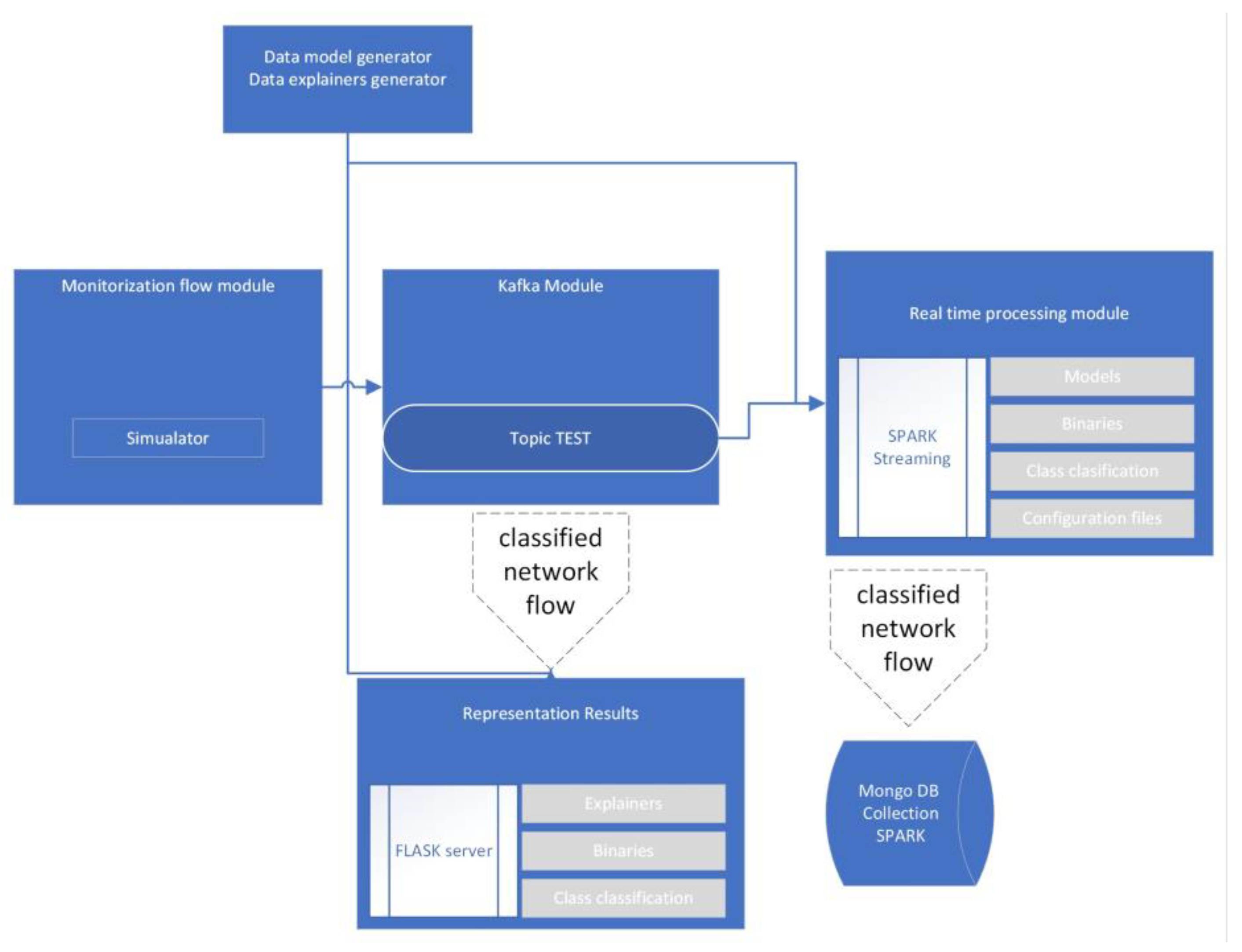
Concurrently, this research additionally introduces a system with the capabilities to utilize an artificial intelligence module for real-time analysis and transmission of received traces, along with their results, for graphical representation and historical recording in a database. The visualization component is designed to display classified data along with their explanations, the aforementioned database, and system customization settings for user personalization.
The system architecture is defined by four primary blocks. These blocks are categorized as trace monitoring, data transmission, real-time processing, and result representation.
3.1. Trace Monitoring
This block is responsible for obtaining and monitoring network traces in real-time based on the UNSW-NB15 data flows. SQL Dataframe objects are compatible with Spark structured streaming dataframes. It captures and preprocesses the network traffic, extracting relevant features and preparing the data for further analysis. The monitoring component ensures that the system can effectively detect and analyze potential intrusions or anomalies in network traffic.
3.2. Data Transmission
This block focuses on the efficient transmission of data between the different components of the system. It facilitates the flow of information from the trace monitoring component to the real-time processing component and then to the result representation component. This block ensures that the data is communicated effectively and securely throughout the system. This block was developed using Kafka [
9].
3.3. Real-Time Processing
This block is responsible for analyzing the network traces in real-time using machine learning algorithms and XAI techniques. It processes the data received from the data transmission component, classifies it as normal traffic or anomalies, and identifies the type of anomaly based on the attacks studied in the UNSW-NB15 dataset. The real-time processing component ensures that the system can accurately and quickly detect intrusions and anomalies in the network traffic.
3.4. Result Representation
This block is responsible for displaying the classified data along with its explanation, allowing users to visualize the detected intrusions and anomalies as presented in
Figure 1. It is based on Mongo DB due to its real-time data storage capacity. Furthermore, a Flask server was utilized for result representation. This database stores historical data and has a configuration interface for user customization. The result representation component ensures that the system’s findings are presented in an understandable and actionable manner for users.
4. Experimentation and Evaluation
In this section, we evaluate the performance of the entire software, beginning with a study conducted to optimize the algorithms of each implemented model type. From the various candidates of each model type, we select the one considered optimal, subsequently verifying the developed explainer generator. After completing this process with all model types. The models were compared for binary and multiclass classification. Finally, the complete functionality was tested using models in the data processing block and their respective explainers in the results representation block.
4.1. Feature Selection Methodology
To compare model types as described in this chapter, it is first necessary to detail the common feature selection methodology based on preprocessing. We have divided it into two stages: first the data normalization and then the data balancing method.
4.1.1. Data Preparation
Initially, for the training dataset, records containing an unknown service, written as “-”, were removed. Next, the features were transformed into their corresponding types, resulting in three categorical features: “proto”, “service”, and “state”. OneHotEncoder [
4] encoding was chosen for these categories.
After preprocessing, we observe different anomaly and non-anomaly distributions for binary classification (
Table 1) and attack distributions for multiclass classification (
Table 2).
4.1.2. Data Balancing Method
Then, the distributions of classes are evaluated. The significant disparity between them indicates that the dataset is unbalanced. An unbalanced dataset implies a substantial difference in the number of records to classify and can negatively impact the model, primarily by causing overfitting. This may mean that our models tend to learn to classify the majority class or classes, ignoring the rest and not affecting metrics such as accuracy. Therefore, the study in the following subchapters is conducted with the unbalanced or non-balanced (SB) dataset and the balanced (B) dataset to observe which models perform more effectively.
To balance the dataset, we opted for oversampling, which involves duplicating samples from minority classes to match those of the majority classes. For this process, multiple methods based on mathematical correlations of the attributes with the target label were analyzed, such as Kendall, Pearson, or Spearman correlation. Kendall correlation was used, which is a non-parametric method that utilizes the ranking of observations. It is similar to Pearson’s correlation but is more commonly employed when parameters are not standardized, making it important to highlight the following information:
The correlation result ranged between 1 and −1 (perfect positive correlation and perfect negative correlation);
They were used as a measure of the strength of association between two variables, meaning they quantified the effect size. It can be said that a value of 0 is a null correlation, between 0.1 and 0.3 a (0.1–0.3) small association, between 0.3 and 0.5 a (0.3–0.5) medium correlation, between 0.5 and 0.7 a (0.5–0.7) moderate association, and higher a high or very high association. Using the Pandas library, correlation matrices were obtained for the four possible combinations by selecting the associated features from the proposed ranges.
Upon applying the previously mentioned methodology, coefficients greater than 0.45 were selected for both balanced and unbalanced datasets for binary classification. For the multiclass classification approach, a coefficient greater than 0.75 was chosen for the unbalanced dataset due to the high correlation factor between the features. Moreover, for the balanced dataset, a coefficient greater than 0.22 was selected due to a low correlation factor between the features. The selected metrics are the following for each of the mentioned datasets:
Binary class (B): dinpkt, ct_dst_src_ltm, sbytes, dpkts, dbytes, ct_src_dport_ltm, dmean, ct_dst_sport_ltm, dload, state, sttl, ct_state_ttl;
Binary class (SB): dbytes, dpkt, ct_dst_sport_ltm, dmean, state, dload, ct_state_ttl, sttl;
Multiclass (B): sload, dloss, dload, dbytes, response_body_len, dmean, sttl;
Multiclass (SB): dmean, ct_state_ttl, state_FIN, service_dns, swin, dwin, proto_tcp, proto_udp, dttl, state_INT.
4.2. Algorithms under Study
4.2.1. Decision Tree
The decision tree model was created by modifying various hyperparameters, which affected the different results and training times. In this research, only the max_depth parameter was altered, influencing the number of depth nodes the model could have. Therefore, to have an adequate number of models of this type for comparison, decision trees with 10, 15, 20, and 25 nodes were chosen for each dataset type. The following figures show the results obtained by the no-balanced (B) and no-balanced (SB) datasets. As (SB) and a balanced dataset as (B).
Binary Classification
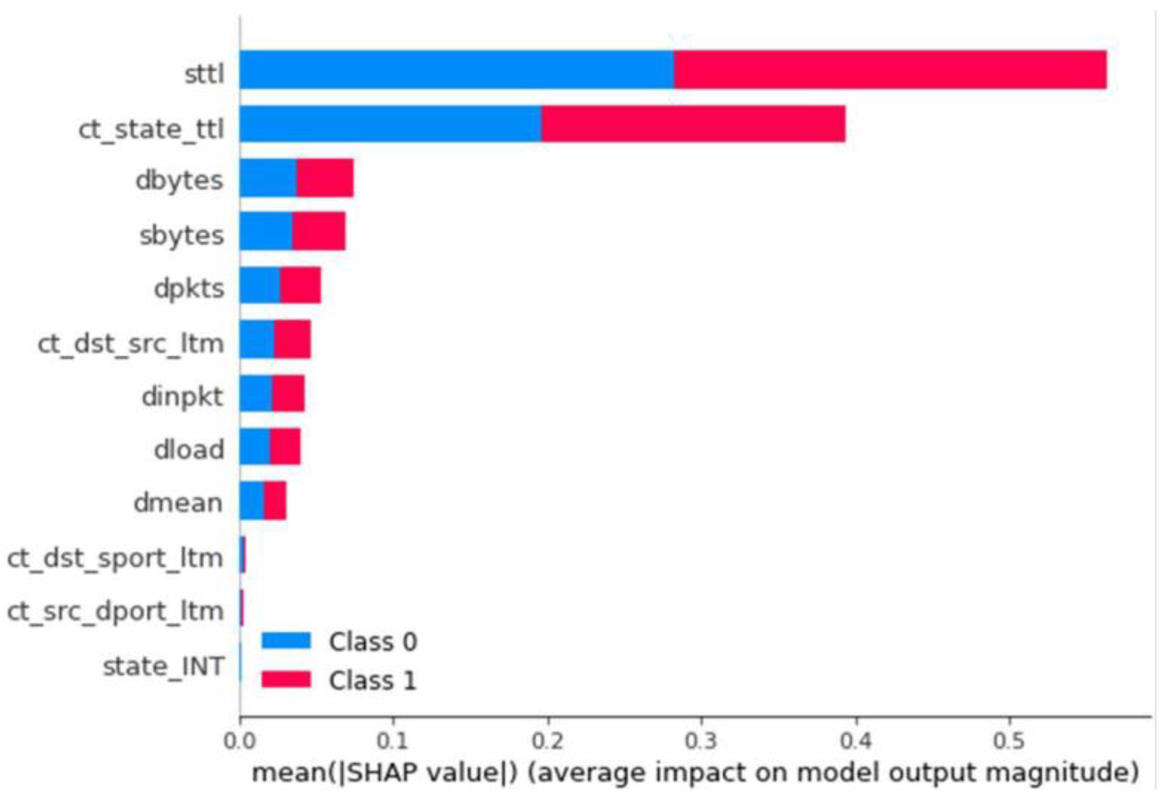
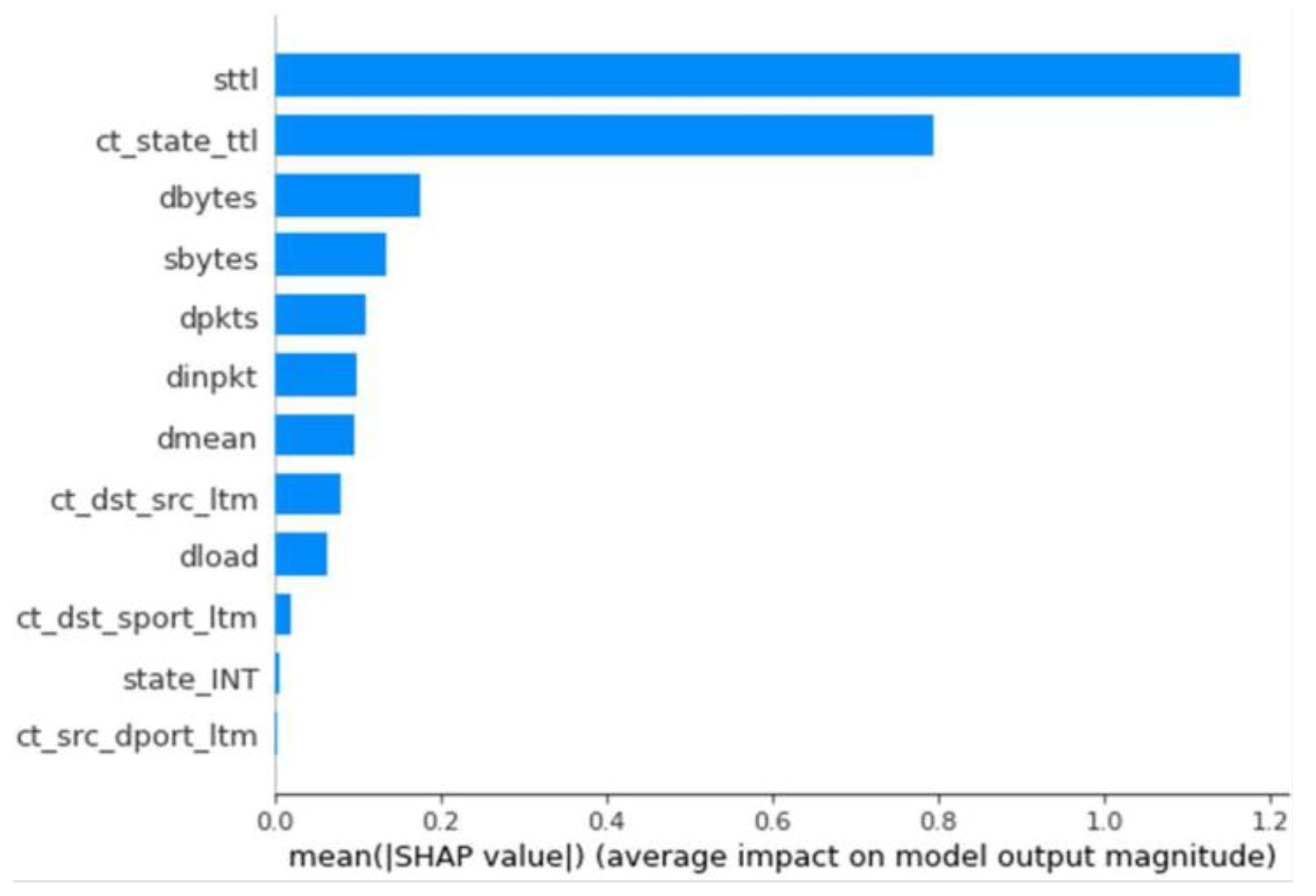
The results for all combinations of parameters and dataset types were found to be quite evenly matched. If we consider the F1 metric as the most important, as it indicates the success rate for anomaly detection combined with the precision for classifying it, several models could be chosen. However, the best model is deemed to be the one configured with a maximum of 25 layers and trained on a balanced dataset due to the number of data points used for attacks. Having chosen this model, it is saved and stored in the real-time processing block under the name “DT”. Once stored, we use the developed explainer generator to create its SHAP value generator. This is saved on the result representation server under the name “DT.” After generating the model, the importance of each feature for classifying anomalies is observed, as represented in
Figure 2. Upon analysis, we can determine the correspondence with the correlation values calculated earlier.
Multiclass Classification
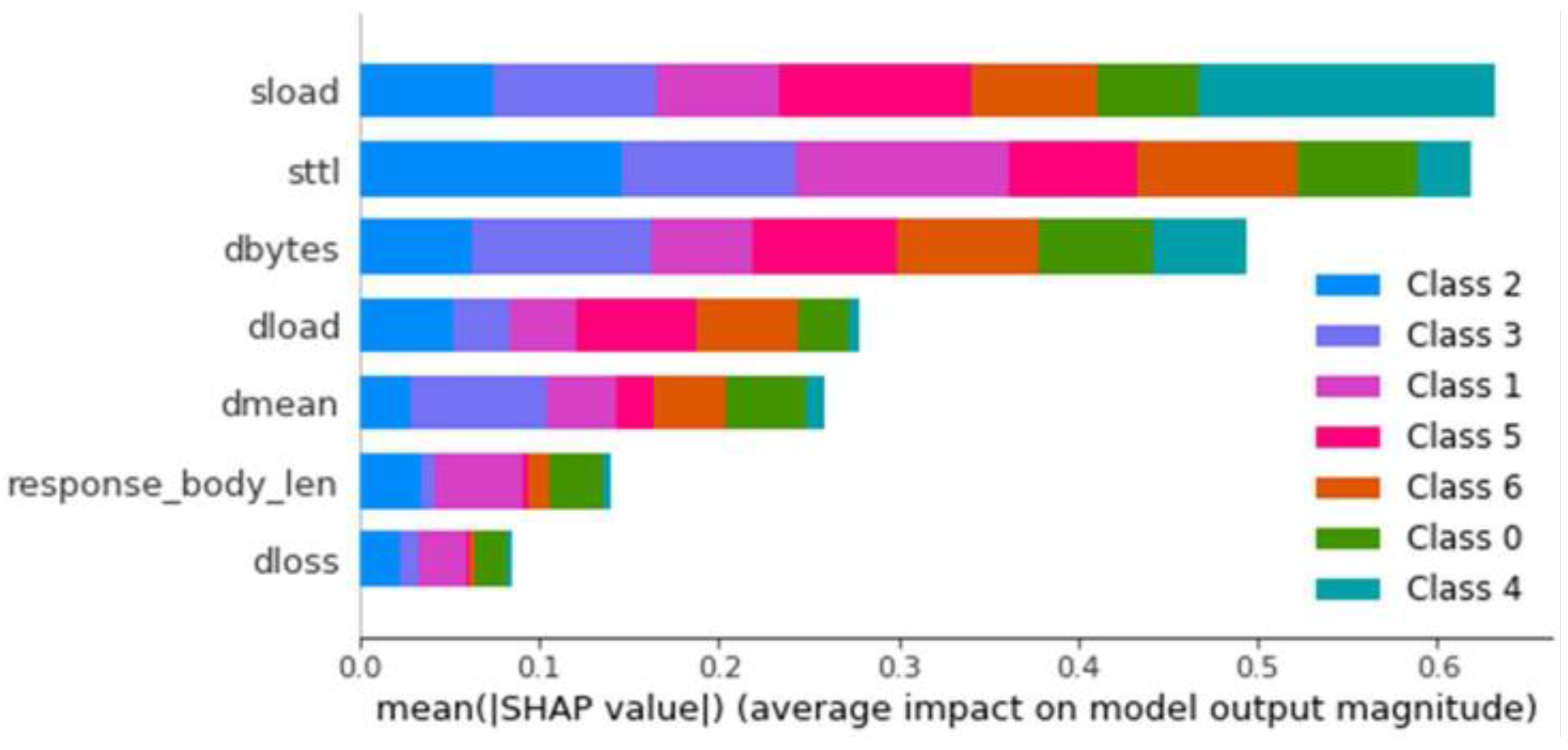
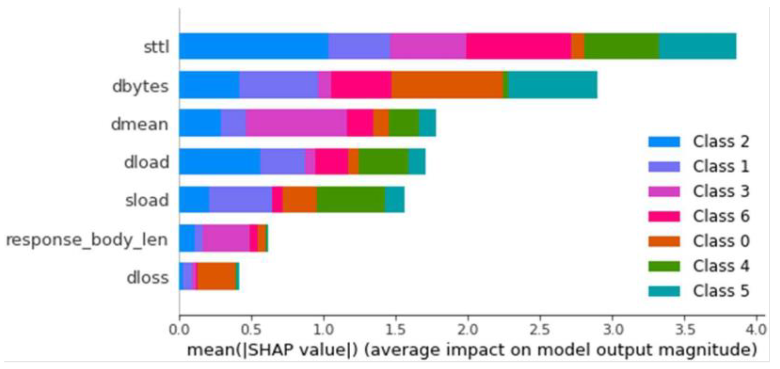
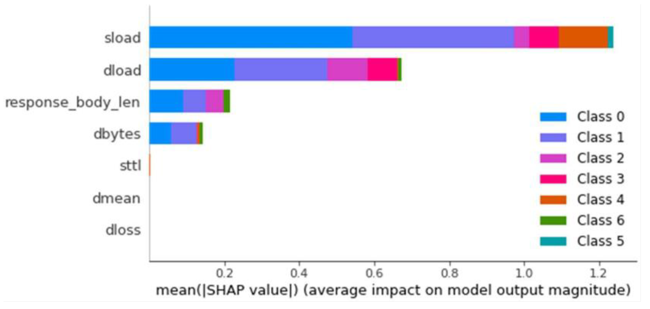
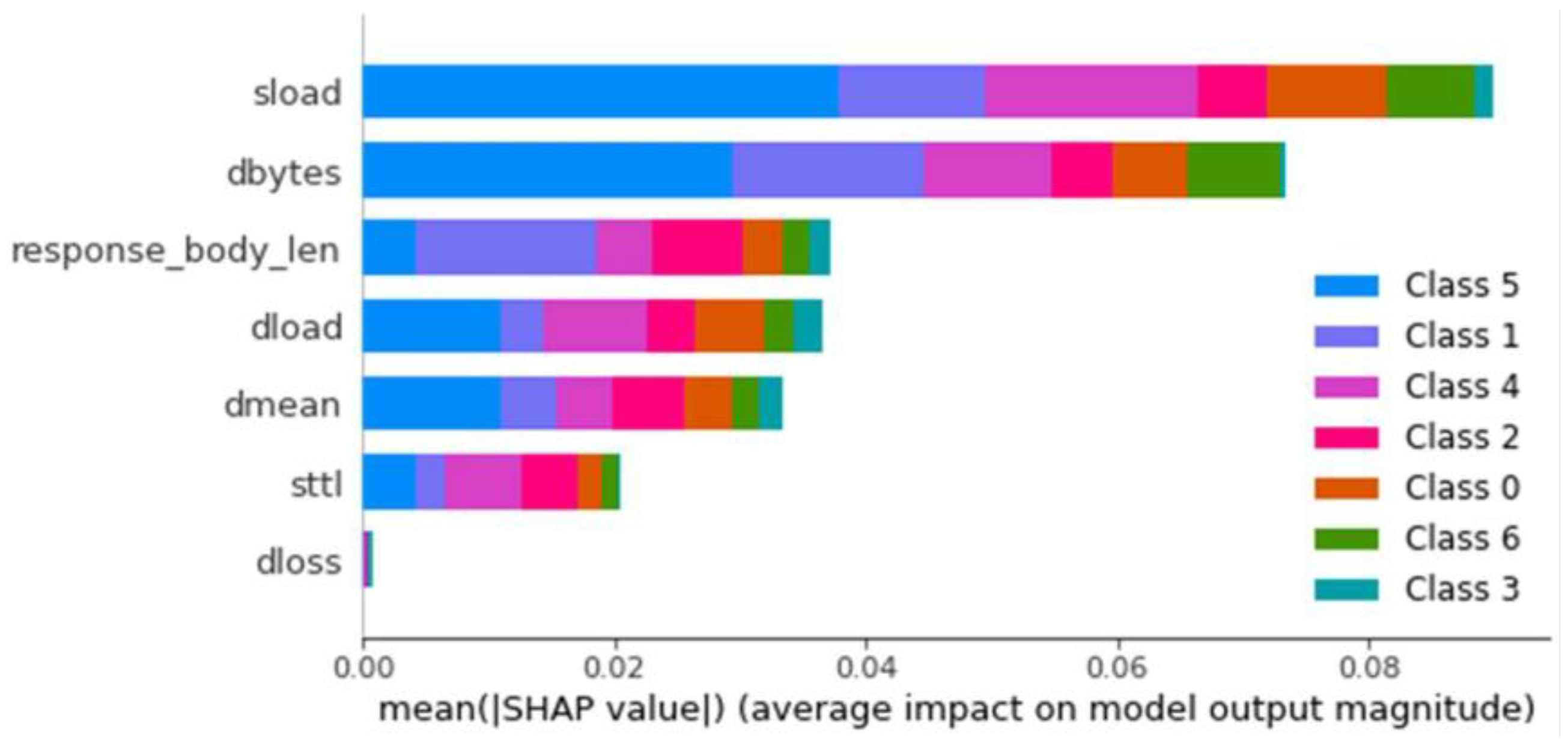
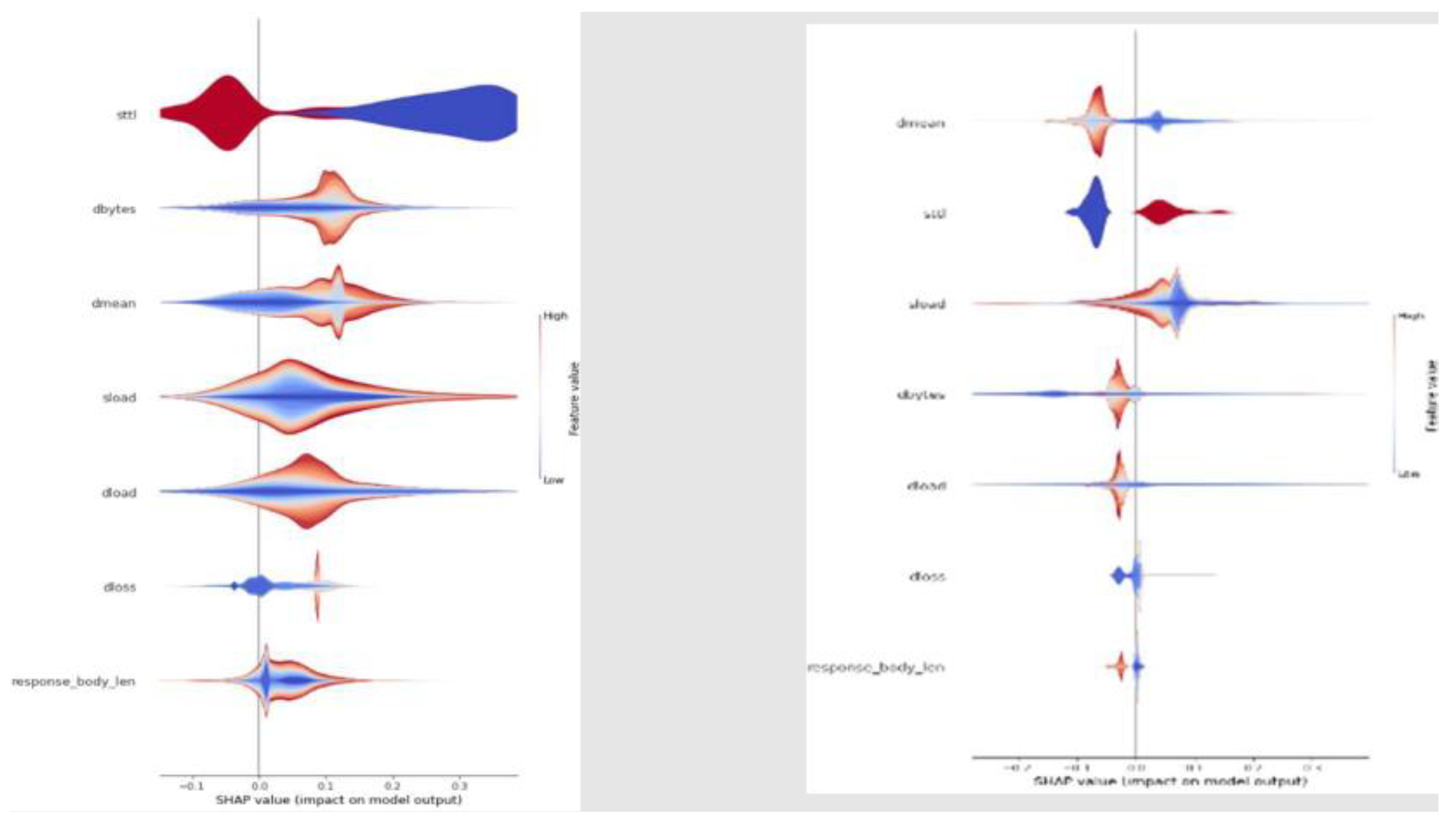
For multiclass classification, the model was also applied to the balanced and unbalanced datasets. To determine the optimal configuration, the average TPR and FPR of all classes were calculated, scoring proportionally from 1 to 0 for the best and worst results, adding the scores obtained for the TPR and subtracting those obtained for the FPR. The models trained with the balanced dataset stand out for their significant advantage in multiclass classification, with the best model being the one created with a maximum depth of 20 layers. The same process as in binary classification is performed, saving the model and generating the explainer. Once generated, it is loaded and observed for this model. The importance of each feature for classifying each type of anomaly is shown in
Figure 3.
4.2.2. XGBoost
The different hyperparameters for the XGBoost model that were analyzed for this model are as follows:
Objective: customize the learning task of the algorithm. Logistic and pairwise were used for binary classification, and Softmax for multiclass classification;
Max_depth: maximum depth of decision trees. The values used are 25 and 20;
N_estimators: number of decision trees within the boosting. The values used were 10, 15, and 40.
Binary Classification
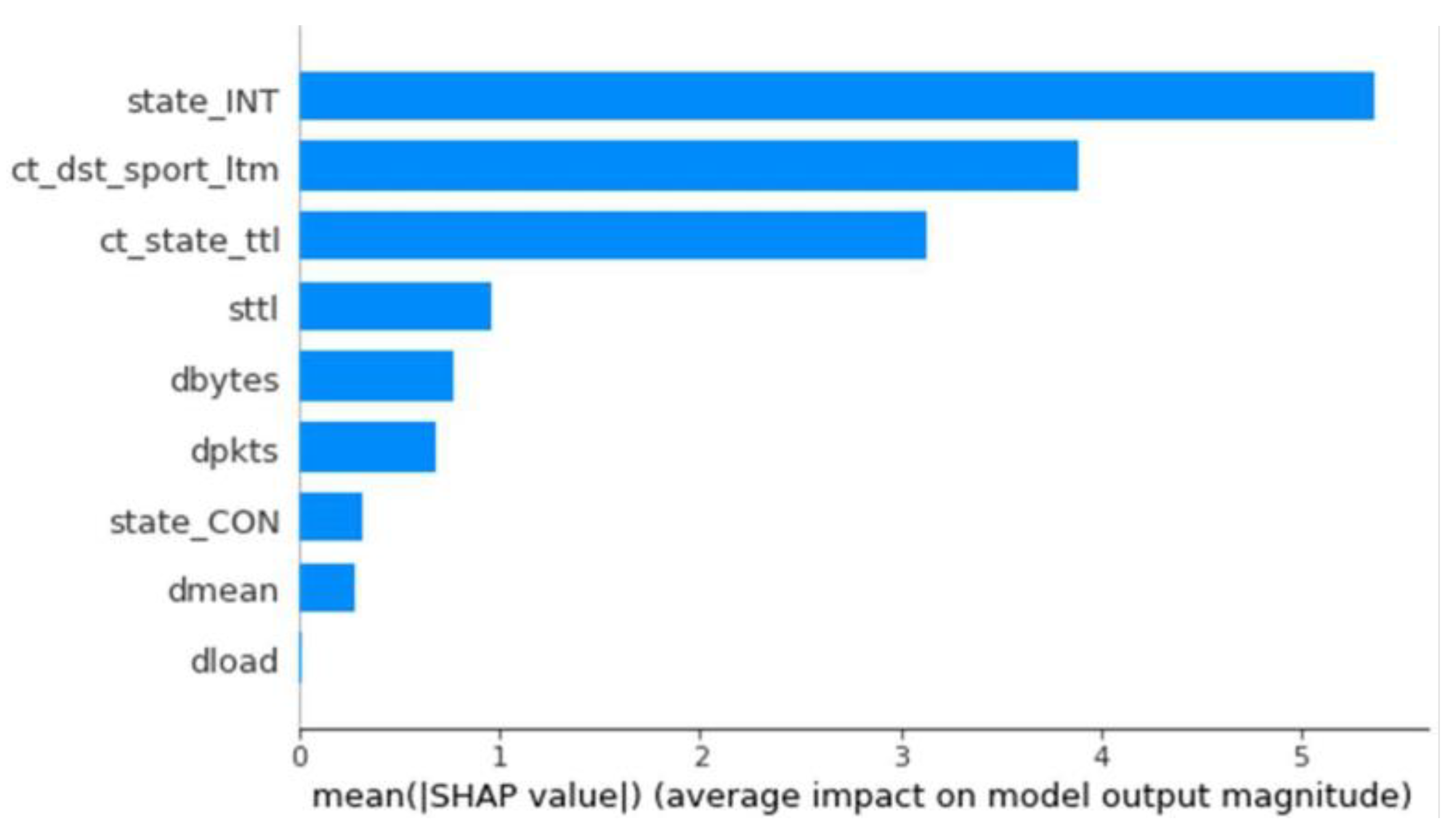
Due to the high average values achieved for binary classification because of the similarity of the metrics in F1, Precision, and Recall, both the model with 15 and 40 estimators with a balanced dataset could be chosen as the best. For simplicity, the model with 15 estimators was selected. Once stored, we use the developed explainer generator to generate its SHAP values. It is saved on the results display server with the name XGB. The influence of each feature for this model is generated for classifying a trace as an anomaly, i.e., with a value of 1 (
Figure 4).
Multiclass Classification
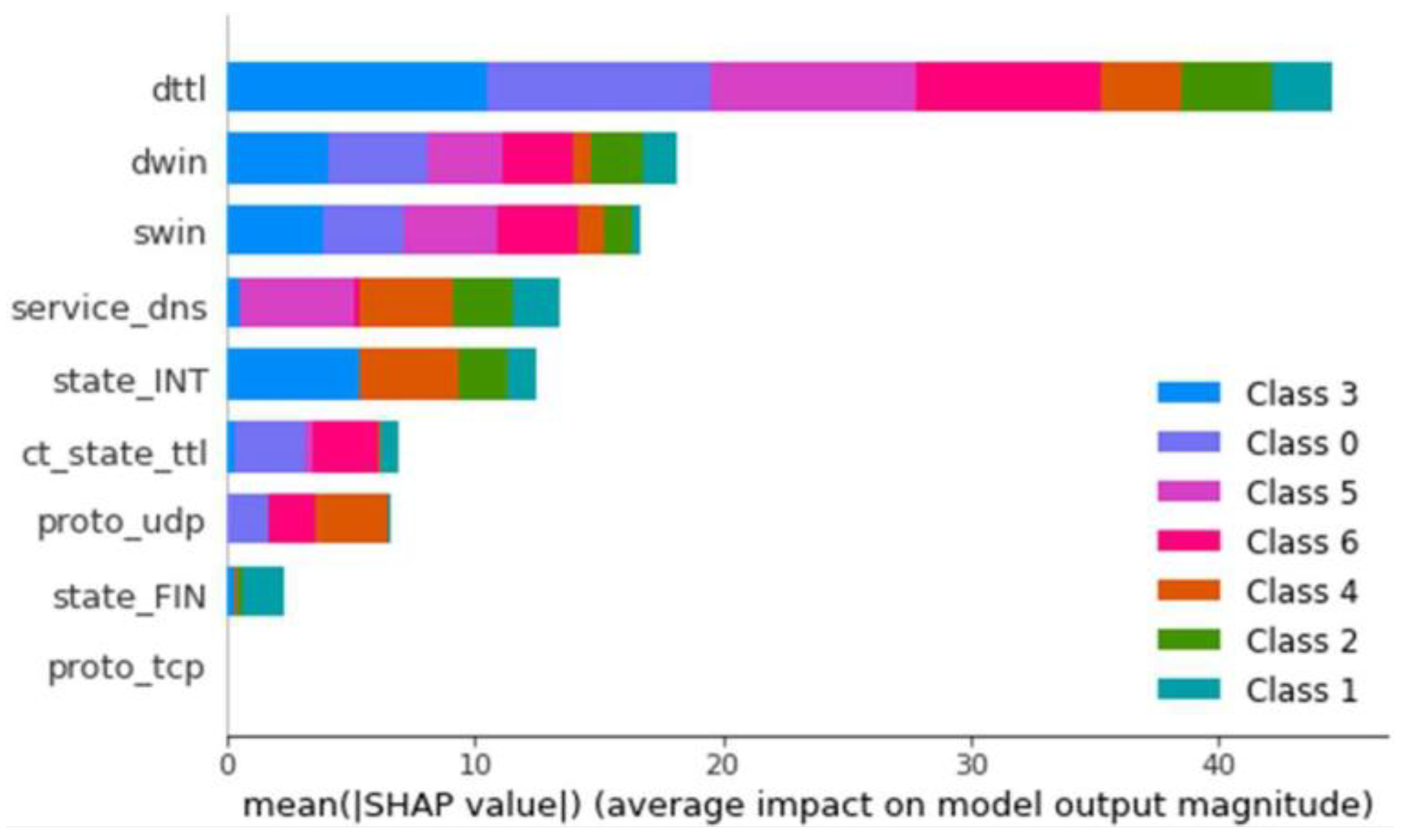
The TPR and FPR values measured for multiclass classification and the balanced and unbalanced datasets for each class in this type of model were analyzed. Using the balanced dataset, much better results were shown for these models, with a primary equality between the models with 40 and 30 estimators. As in the previous case, the model with 30 estimators was chosen for simplicity in training times and model structure. Continuing with the same process as in binary classification, saving the model and generating the explainer, we load and observe for this model the importance of each feature for classifying each type of anomaly (
Figure 5).
4.2.3. Logistic Regression
For the logistic regression model, only two types of models were created, varying the penalty hyperparameter between L1 and L2.
Binary Classification
In this case, the unbalanced model with L1 penalty stands out among the rest with an F1 score of 0.98, an almost perfect Recall, and a Precision value considerably higher than the rest. Once stored, we used the developed explainer generator to generate its SHAP values. It was saved on the results display server under the name LogR (
Figure 6).
Multiclass Classification
The TPR and FPR values measured for multiclass classification and the balanced and unbalanced datasets for each class in this type of model were analyzed. The results were not optimal, but like in the binary case, the best model is the one with the L1 penalty and the unbalanced dataset. Continuing with the same process as in binary classification, the model was saved and the explainer generated. We then loaded and observed the importance of each feature for classifying each type of anomaly for this model (
Figure 7).
4.2.4. KNN
For the KNN model, the number of neighbors ranges between 5, 15, 35, and 75.
Binary Classification
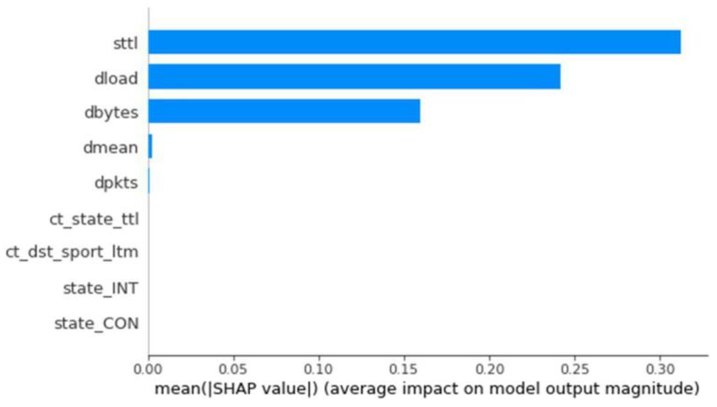
The results for the different combinations and binary classifications were analyzed. In this case, optimal results for F1, Recall, and Precision were obtained for all models, ultimately choosing the model with KNN equal to 5, which displays the highest metrics. Once stored, we used the developed explainer generator to generate its SHAP values. The influence of each feature for this model on classifying a trace as an anomaly was generated, revealing that most features for this model do not have a significant influence, except for Sttl, Dload, and Dbytes (
Figure 8).
Multiclass Classification
The TPR and FPR values measured for multiclass classification and the balanced and unbalanced datasets for each class in this type of model were also analyzed. As in binary training, the best model is one with K equal to 5, but this time with a balanced dataset, significantly outperforming the other options with the highest TPR and the lowest FPR. Continuing with the same process as in binary classification, the model was saved and the explainer generated. We observed the importance of each feature for classifying each type of anomaly in this model. In this case, Dmean, Dloss, and Sttl do not have great relevance for classification despite the relevance these features provide in the Kendall linear relationship (
Figure 9).
4.2.5. Random Forest
The random forest (RF) model was developed by modifying different hyperparameters, which vary the results and training times. In this experimentation, we adjusted the max_depth parameter, which influences the number of depth nodes that the model can have, and the criterion parameter, alternating between Gini and Entropy. Therefore, to have enough models of this type for comparison, random forest models with 50, 100, 150, and 200 nodes were tested for each type of dataset.
Binary Classification
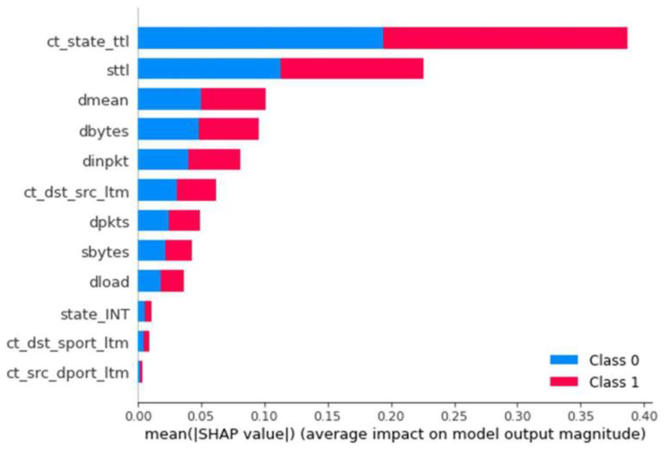
The results for all parameter combinations and dataset types are very similar. Considering the F1 metric as the most important, all models have similar values in the other metrics as well. However, due to the precision, accuracy, and simplicity of the number of nodes, the model with 50 nodes and the entropy criterion was chosen. Once stored, we used the developed explainer generator to generate its SHAP values. The importance of each feature for classifying an anomaly or not was loaded and observed for this model (
Figure 10).
Multiclass Classification
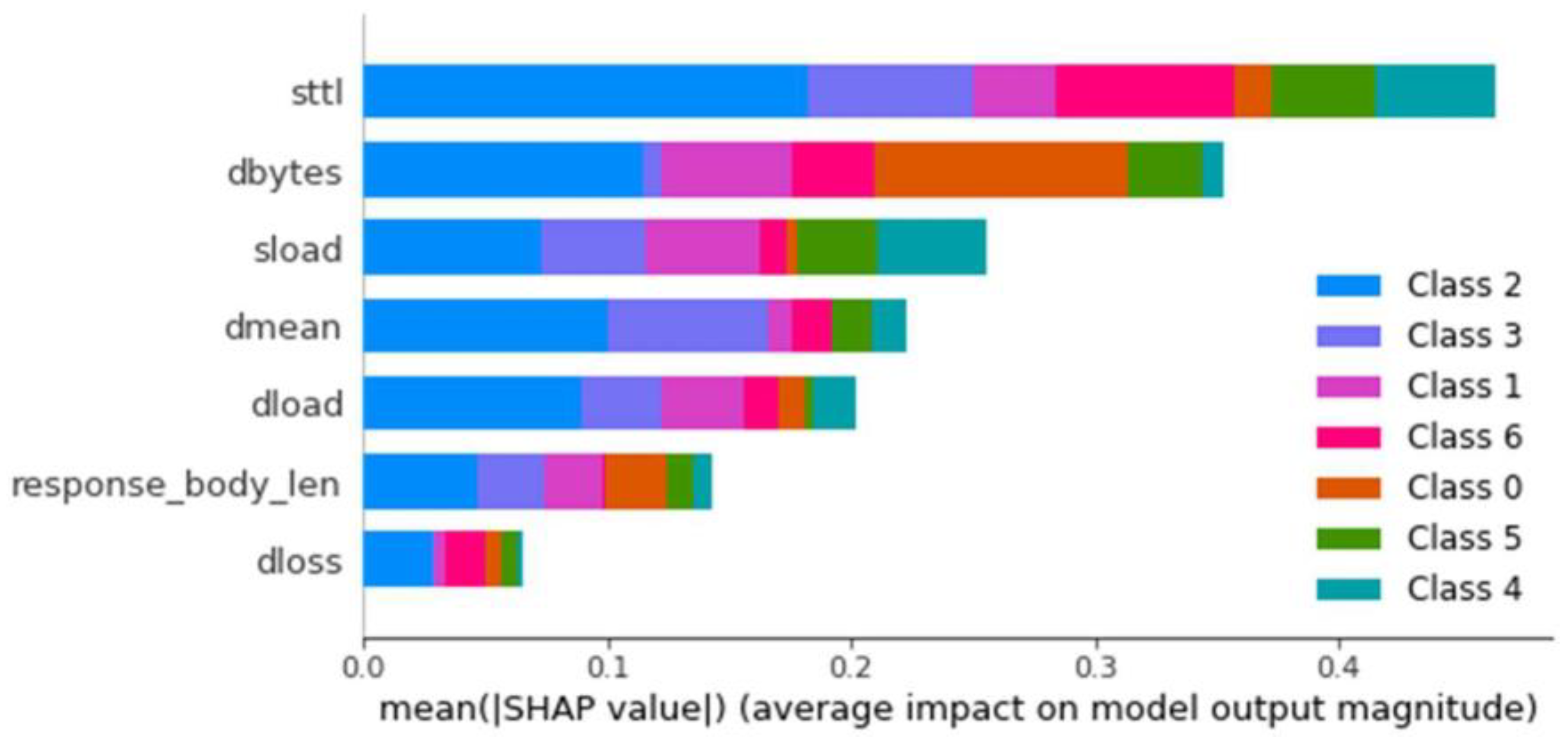
In this case, it is noteworthy that the models trained with the balanced dataset show a significant advantage in multiclass classification. All the tests done presented similar values, and therefore, following the same criterion as in binary classification, the model with 100 nodes and the Gini criterion was chosen for simplicity. The same process as in binary classification was carried out, saving the model and generating the explainer. Once generated, the importance of each feature for classifying each type of anomaly was loaded and observed for this model (
Figure 11).
4.2.6. Multi-Layer Perceptron
For the multi-layer perceptron (MLP) model, the configuration of essential hyperparameters primarily involves defining the model’s layer structure. Mathematical equations and layer numbers observed in various works were employed, and different combinations were tested. The structure defined in the work [
23] was followed, using architectures with four hidden layers in some cases and the following neuron calculations:
Hidden Layer 1: 0,75 · Input Neurons + Output Neurons;
Hidden Layer 2: (Input Neurons + Output Neurons)/2;
Hidden Layer 3: 70% Input Neurons;
Hidden Layer 4: 90% Input Neurons.
Binary Classification
For binary classification, two models with proper functioning were used for both balanced and unbalanced datasets: one with a single hidden layer of 100 neurons and another with two hidden layers of 50 neurons. Following the calculations previously explained, it is essential to recall that binary models with unbalanced datasets have nine input features and balanced datasets have 12. Consequently, two additional models were calculated for each type, varying the rounding given by the equation results.
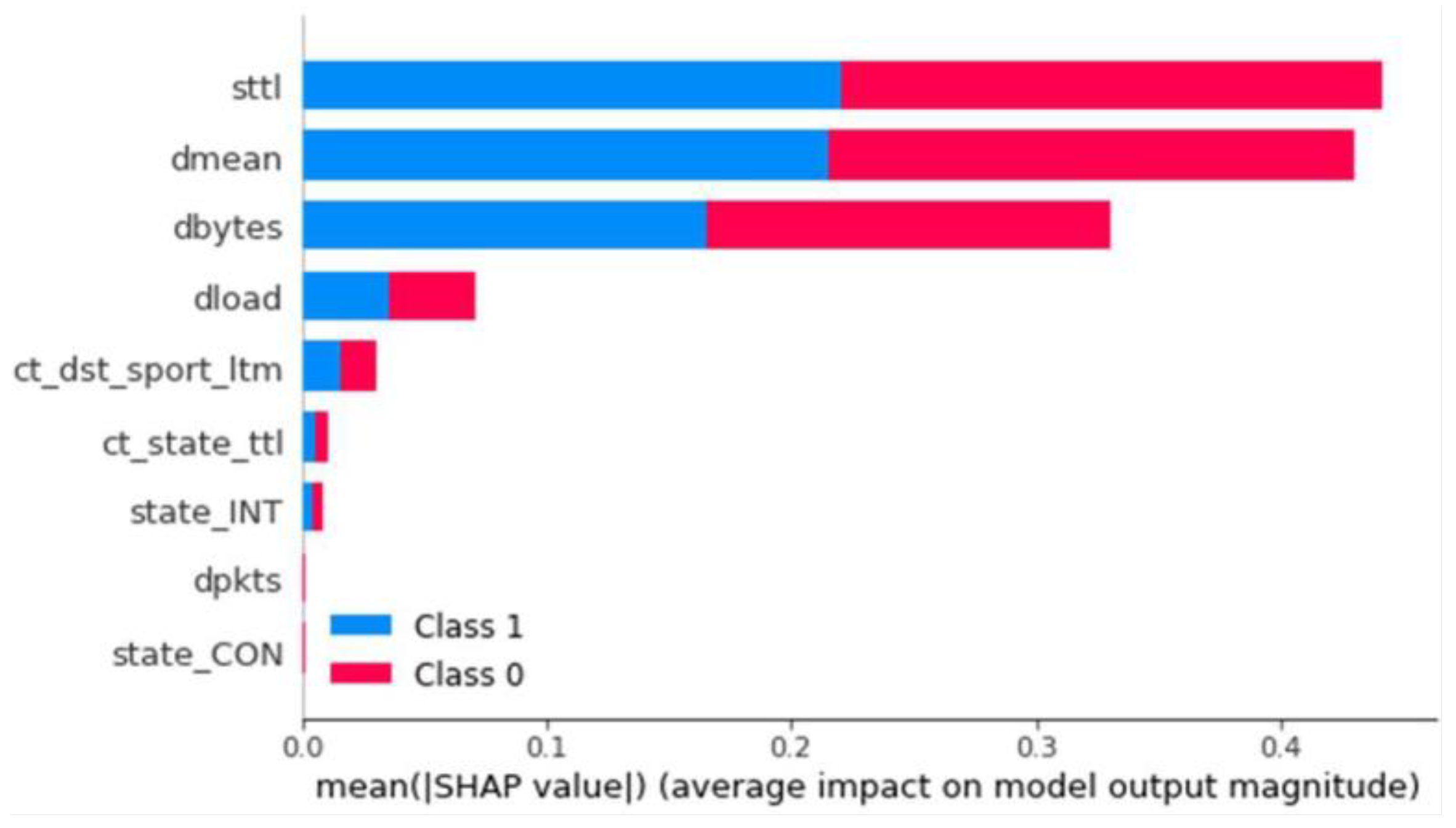
On this occasion, optimal F1, Recall, and Precision results were obtained for all models. However, there was a significant dispersion in most cases when one metric was very high compared to the others. The model trained with the unbalanced dataset with two hidden layers of 50 neurons maintained the highest values for all three measures. Once stored, the explainer generator was used to generate the SHAP value generator for the model. It was saved on the result representation server under the name MLP. The influence of each feature for this model in classifying a trace as an anomaly or not was generated. It can be observed that Sttl, Dmean, and Dbytes have a significant impact (
Figure 12).
Multiclass Classification
For multiclass classification, two models with proper functioning were used for both balanced and unbalanced datasets, similar to binary classification. Following the calculations previously explained, it is essential to recall that multiclass models with unbalanced datasets have ten input features and balanced datasets have seven. Consequently, two additional models were calculated for each type, varying the rounding given by the equation results. According to the scoring system, there is a clear advantage to the balanced model with a single hidden layer of 100 neurons. Continuing with the same process as in binary classification, the model was saved, and the explainer was generated. The importance of each feature for classifying each type of anomaly was loaded and observed for this model (
Figure 13).
Table 3 summarizes the configuration of the neural networks for the different models. Each row represents a model, and the columns provide information on the number of hidden layers and neurons in each layer.
In summary, the various combinations and results for both binary and multiclass classifications were analyzed, and the most effective models were identified. The influence of different features on the classification was also examined, highlighting key features that significantly impact the classification’s performance. The selected models and their corresponding explainers were saved and implemented for further use in the application.
4.2.7. Choice of the Best Model
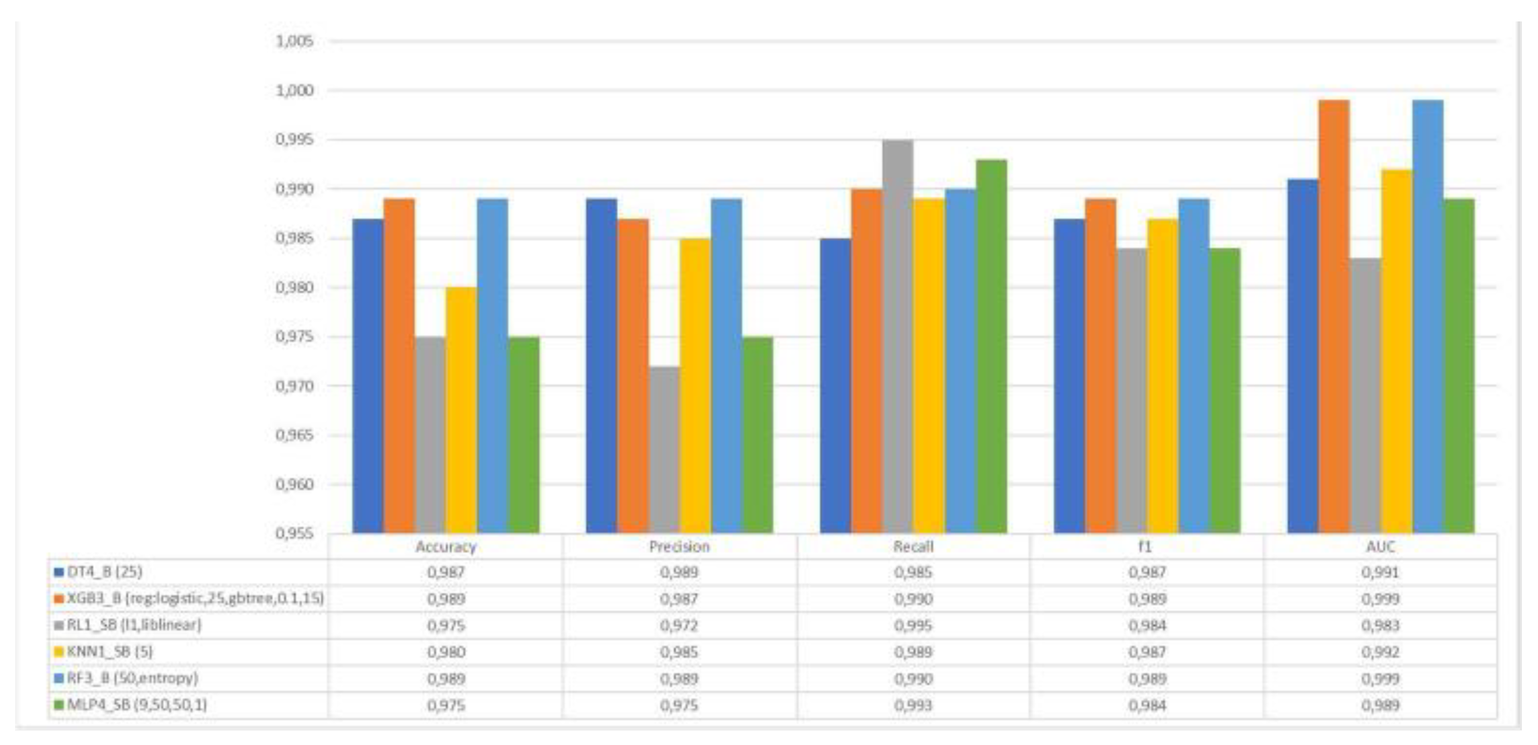
Once the analysis was completed and the best model of each type was chosen, an evaluation was performed to determine the optimal model for binary and multiclass classification. Furthermore, a comparison of the SHAP values of the models was conducted to observe the relationships and conclusions of the various attributes used. As for binary classification, a comparison of the models can be seen in
Figure 14.
Upon analyzing the results, similar values were observed for most metrics. However, the model with the highest values in Precision, Recall, and F1 was the random forest, which was subsequently chosen for the XAI model. Continuing with the SHAP values observed in previous sections, models with the same characteristics were compared, specifically those trained with the balanced dataset. These models were decision tree and XGBoost, both of which had nearly identical SHAP values, with significant importance placed on the
Sttl and
ct_state_ttl features. On the other hand, the SHAP values for anomaly classification in the random forest model showed a different importance, with very high and even values among the
Dbytes, Dmean, Dintpkt, ct_state_ttl, Sbytes, and
dload features. This result could indicate that the model is more stable due to the greater influence of multiple features, meaning it uses more information from the traces and does not primarily depend on two fields of information. This is illustrated in
Figure 2,
Figure 4, and
Figure 10.
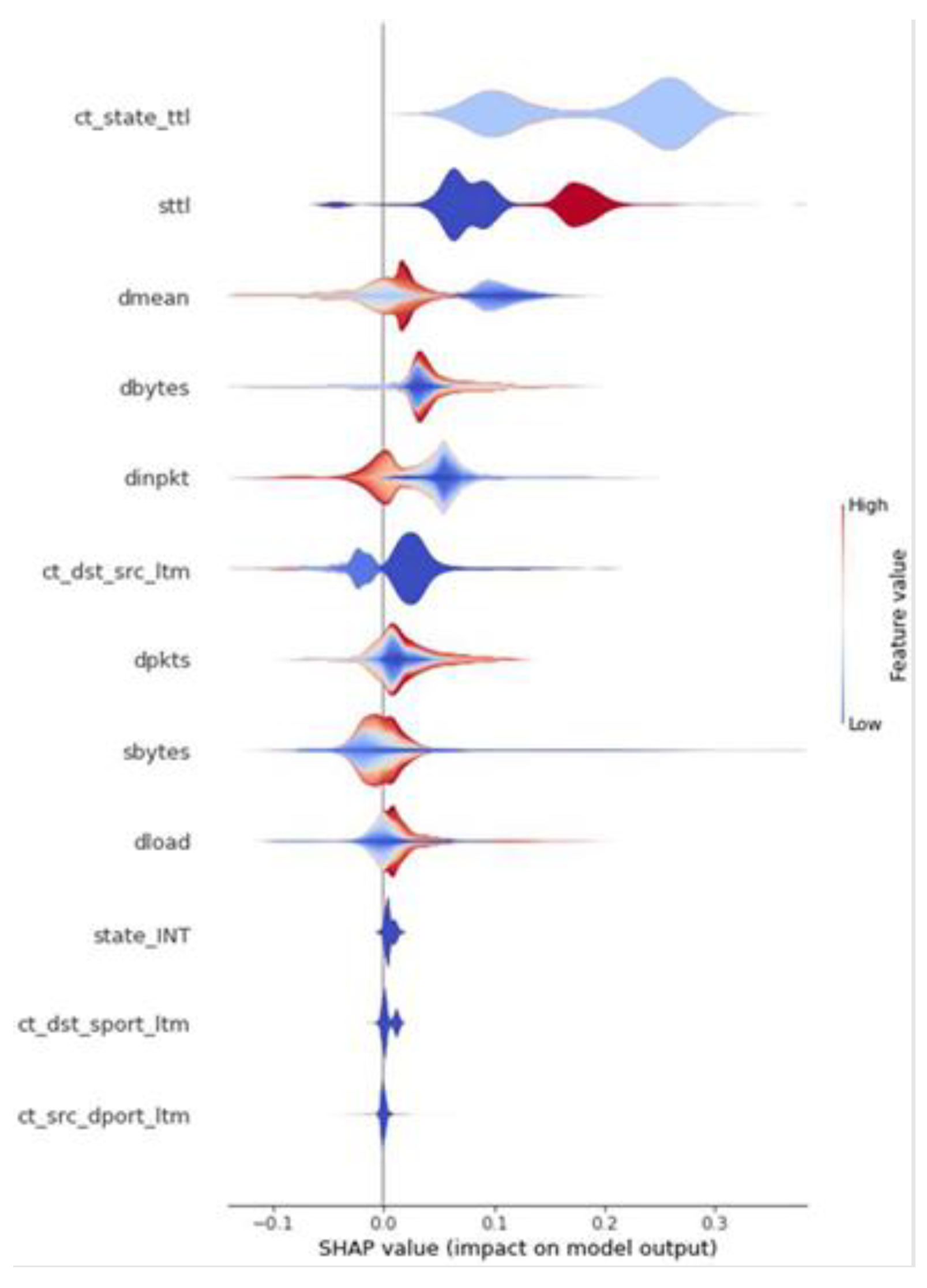
Figure 15 represents the sensitivity of the different features for identifying an anomalous trace, helping to better understand the chosen model for demonstration.
Several conclusions can be drawn from the most important features, which can be compared with the real-time performance validated in
Section 4.2:
Ct_state_ttl: A relatively low value directly influences the classification of a trace as an anomaly;
Sttl: An extremely low value influences the classification as an anomaly, but an extremely high value influences it to an even greater extent. This indicates that extreme values in this field are crucial for classifying a trace as anomalous;
Dmean: It can be observed that a range of average or slightly low values to the highest possible values does not influence the labeling of a trace as an anomaly or only slightly influences the classification as normal traffic. However, very low values significantly influence the classification as an anomaly;
Dbytes: Average or slightly low values compared to the average influence the classification of the trace as not normal, while high or extremely low values considerably influence the classification as abnormal traffic;
Dinpkt: From slightly above average values to the lowest possible values, the influence for classifying as anomalous traffic is observed. Values outside this range have little or no influence on classifying the trace as anomalous.
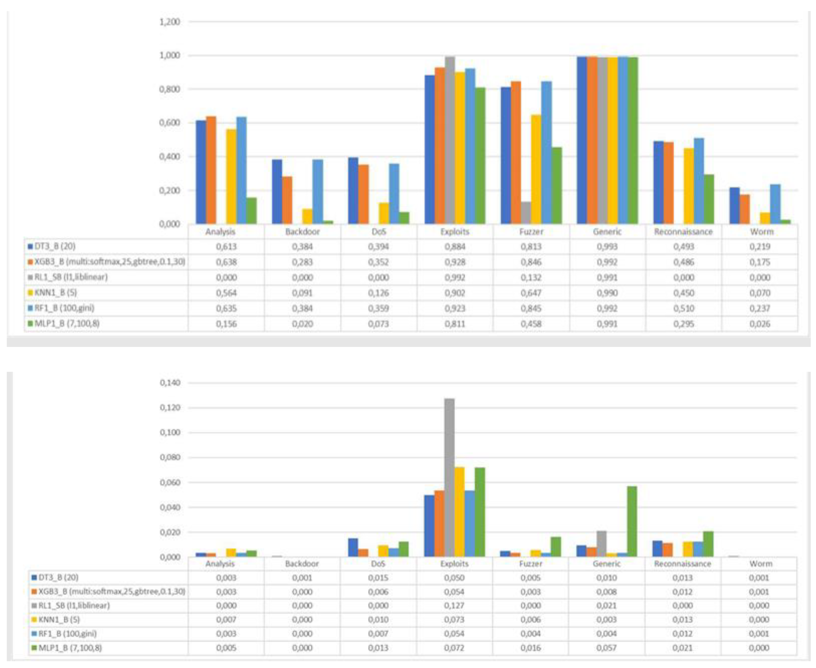
After selecting the model for binary classification, the best model for anomaly-type classification was chosen when a trace was classified as non-normal behavior. For this study,
Figure 16 was used, comparing the TPR and FPR values of the models.
Due to the relatively similar values across all models, the system used in previous sections could not be followed. For this reason, the average TPR and FPR values were calculated as shown in
Table 4.
The MLP, logistic regression, and KNN models were discarded due to their low average TPR values compared to the remaining models. For the three remaining models, the difference between their TPR and FPR values was calculated to determine the most comprehensive model, with random forest emerging as the best model for multiclass classification. Following the same procedure as in binary classification, a similar analysis for each class can be obtained. As an example, the classification of an anomalous trace as a DoS attack or exploit is studied in
Figure 17. It is noteworthy that an extremely low value for the
Sttl attribute is crucial for classifying an attack as DoS, while an extremely high value prevents it from being classified as such, with the opposite behavior for
Exploit-type attacks.
5. Interface Visualization
As a last step, we will validate the final software performance with simulated network traces created from the validation test, predicting in real time with the best model obtained for binary and multiclass classification. Finally, the record stored in the database is shown together with the representation of results available to the user and the corresponding explanation for each prediction.
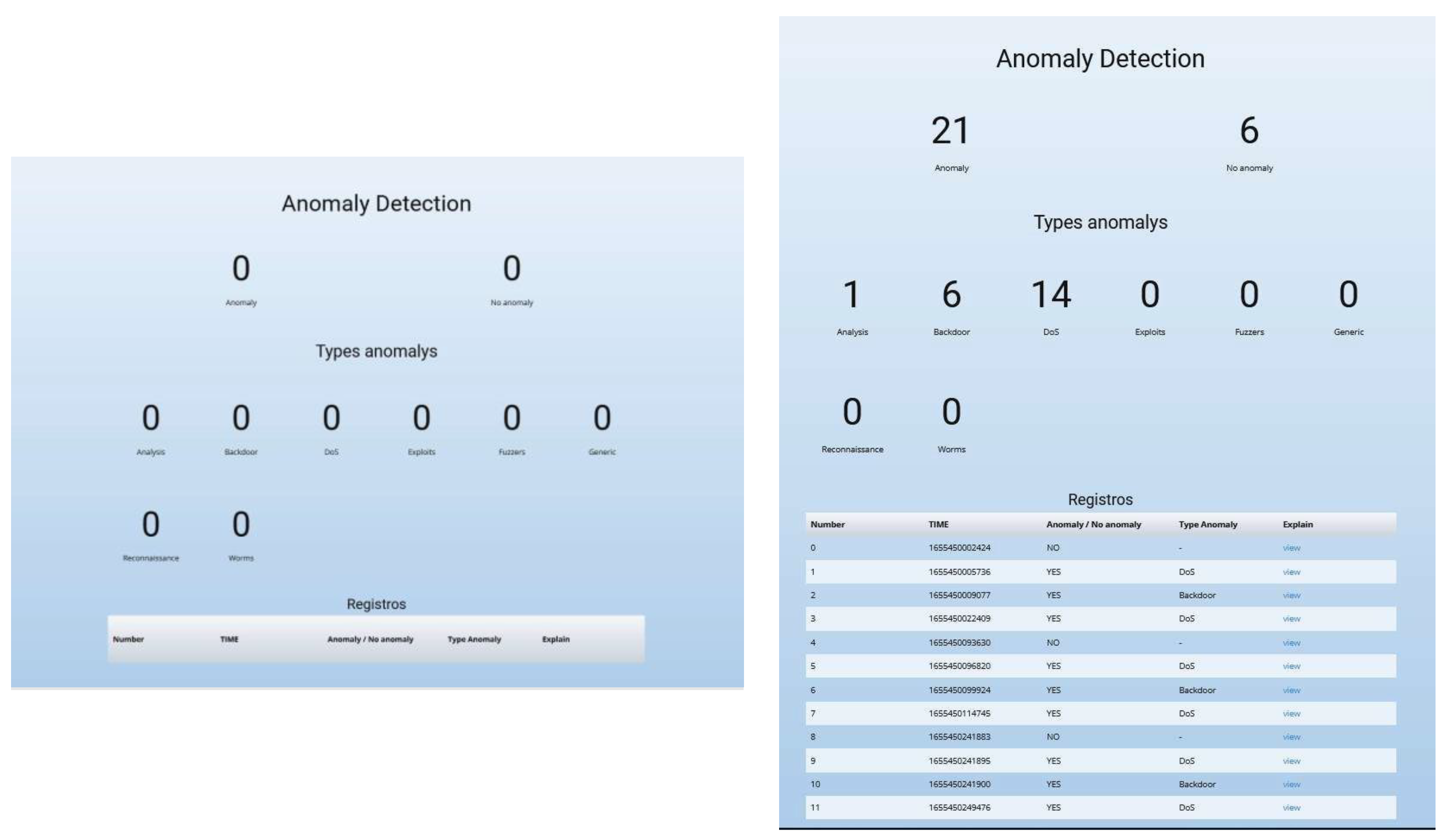
When starting the trace simulator, we observe that some anomalies are received and detected (
Figure 18).
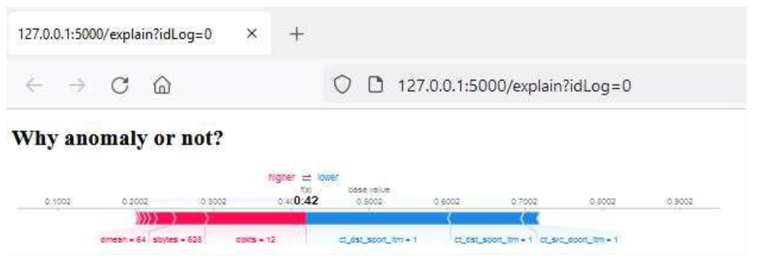
First, we will check a trace classified as normal traffic (
Figure 19), where it can be seen that for this prediction, the Dmean field, Sbytes, and Dpkts are the main reasons why it has been classified as normal traffic.
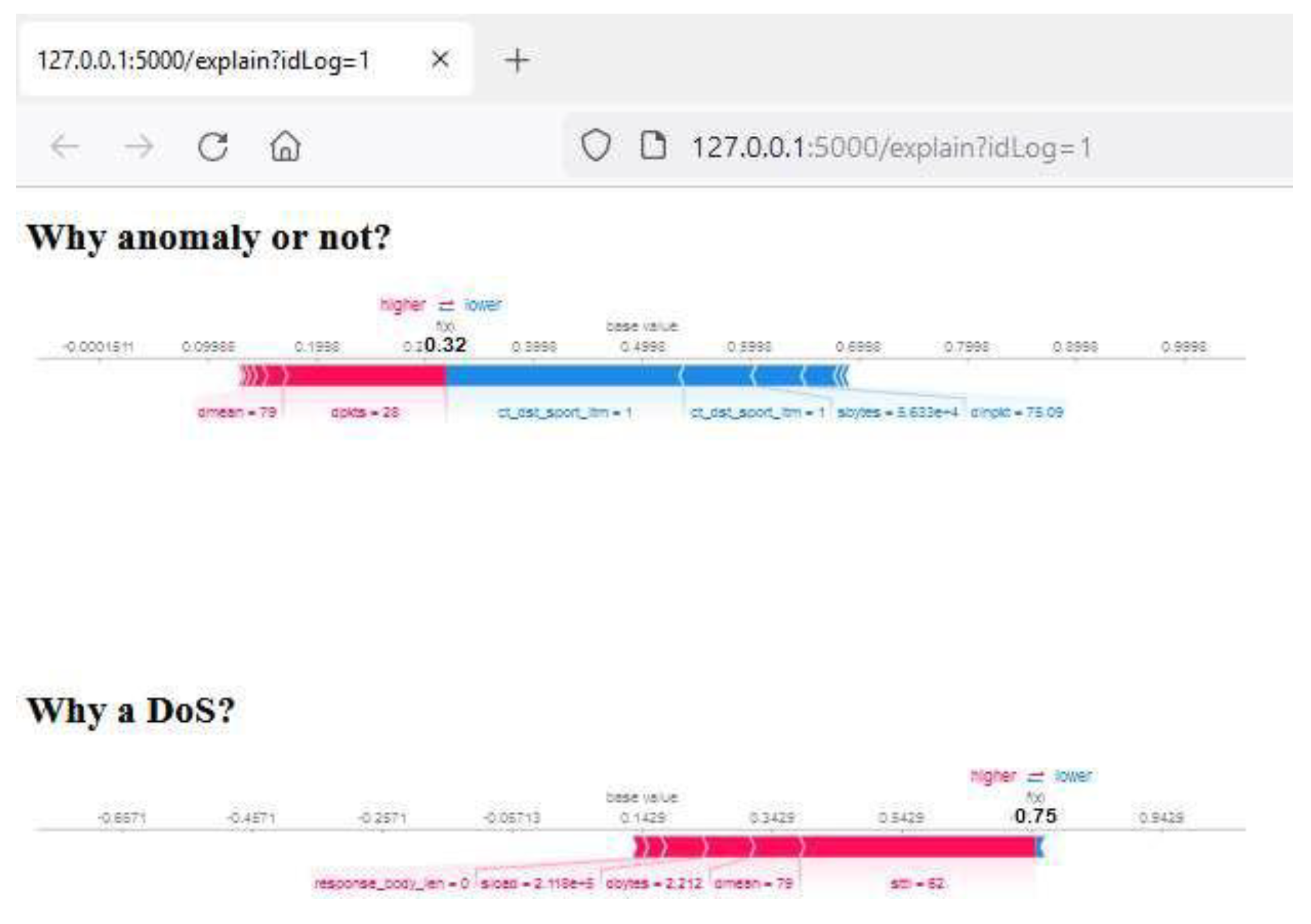
Another example of a trace classified as DoS (
Figure 20) shows that the trace has been classified as anomalous by the Dmean (79) and dpkts (28) fields, while it has been classified as a DoS attack by the values of all fields, having a rather high total SHAP value.
6. Conclusions and Future Lines
The aim of this research was to create a reliable IDS using machine learning, while integrating the function of providing useful explanations for users without necessarily being experts in the field of artificial intelligence. To this end, a modular system was created to monitor traces and analyze them in real time with a choice of certain machine learning algorithms linked to a representation of the results, with statistics and explanations of each classification. To this end, the reliability and confidence of the algorithms have been studied by performing different metric measurements and checks, observing combinations of hyperparameters, and preprocessing and modifying the UNSW-NB15 dataset. The software uses the Spark distributed data processing tool, allowing communication between the different elements in real time through Kafka. This IDS has eliminated the machine learning limitation that Spark’s MLlib library currently has by using different coding tools and thus using specific Python libraries for Artificial Intelligence, such as Sklearn, without losing functionality. Finally, the explanations of this proposal have been achieved with one of the most commonly used tools for XAI, such as SHAP. With it, we have studied the importance of the classifications that have the different values of each feature of the different traces and represent the explanations graphically for each individual prediction in a Flask server. As for the best algorithm found of all the combinations and types evaluated, the best results were obtained with the random forest model.
With this model, it has been determined thanks to explanatory artificial intelligence that some of the most important characteristics are ct_state_ttl (relationship between state and dependency of the protocol used with the lifetime), Sttl (lifetime from source to destination), Dmean (average number of packets transmitted by the destination), or Dbytes (transaction bytes from destination to source). In addition, optimal metrics have been achieved compared to the related research, considering that many do not allow real-time classification, both binary and multi-class classification, and the explanation of each respective model. We have included static classification in the comparison to validate the results of the optimal model obtained in this research. Although it is not performed in real time or using the same algorithm, we believe that it provides a general overview of this approach in comparison to related research in the same area. Due to the high computing resources required for the SVM algorithm, we do not compare the results obtained by this algorithm. This comparison is presented in
Table 5.
In this research, different technologies and tools have been used to create an IDS with explanatory artificial intelligence while maintaining user customization functions, with the priority of offering modular software for the separate improvement of different key components without losing the final operation of the system in a software-spaced design to be deployed in a real system [
7]. For this reason, there are several points that could be improved or extended in each block to provide more complete functionality to the user.
The trace monitoring block is the component that can be updated and improved the most using real tools such as Zeek or Bro-IDS, as explained throughout the research, to obtain real information from a network point, classifying the different characteristics necessary for the operation of the system.
If we continue with the next big component of the research, the data processing block, it is the main container of the Spark executor script, with different points that can be improved or extended to provide greater functionality. As a first phase, increase the number of models available, including others as SVM (support vector machines) or combinations of algorithms for Stacking model assembly types, which were not carried out due to the computational capacity and simplicity of the research. Another feature to be studied in a possible continuation is increasing user customization of the pre-processing performed on the dataset with different normalizations or encodings. Finally, an important functionality to add would be to connect the explanatory module hosted in the results visualization block to calculate the SHAP values directly in the Spark script, thus improving the performance of the system.
In the last module of the research, the results representation block, there are three functionalities that could be updated or added: Firstly, an improvement in the presentation of results in a more detailed way, if necessary. Secondly, a functionality to allow adding a static option to choose local records stored in the MongoDB database and displaying them in the same way as the real-time traces. Lastly, an improvement of the representation of the results of the explanation of each trace, a more textual way of explaining why each prediction has been made without the user needing to understand the graphs, together with the aggregation of different visualizations that the SHAP library allows, with even more complex and exact explanations available for the models.
Finally, the system would benefit from an anomaly alarm system with real-time warning to the user or, as for the studied default machine learning models, an improved cleaning of the dataset that allows the individual improvement of the TPR metric of the multiclass classification and thus avoids false alarms. Also, these same models can be trained by combining different datasets to increase the information on the types of attacks and traffic classified as anomalous that the network can receive, creating a more robust and secure IDS system.
Author Contributions
Conceptualization, X.L.-N. and C.S.-Z.; data curation, C.S.-Z.; formal analysis, X.L.-N., C.S.-Z. and V.A.V.; funding acquisition, V.A.V.; investigation, X.L.-N. and C.S.-Z.; methodology, X.L.-N.; project administration, V.A.V.; resources, X.L.-N.; software, X.L.-N. and C.S.-Z.; supervision, V.A.V., A.M.-L. and J.B.; validation, X.L.-N., V.A.V. and A.M.-L.; visualization, C.S.-Z.; writing—original draft, X.L.-N. and C.S.-Z.; writing—review and editing, X.L.-N., C.S.-Z., V.A.V., A.M.-L. and J.B. All authors have read and agreed to the published version of the manuscript.
Funding
This research received no external funding.
Institutional Review Board Statement
Not applicable.
Informed Consent Statement
Not applicable.
Data Availability Statement
All datasets are available in the mentioned references.
Acknowledgments
Our thanks to Roberto Ríos Guzmán for being part of this research project.
Conflicts of Interest
The authors declare no conflict of interest.
References
- Kovač, A.; Dunđer, I.; Seljan, S. An Overview of Machine Learning Algorithms for Detecting Phishing Attacks on Electronic Messaging Services. In Proceedings of the 2022 45th Jubilee International Convention on Information, Communication and Electronic Technology (MIPRO), Opatija, Croatia, 23–27 May 2022; pp. 954–961. [Google Scholar]
- Mohammadhassani, A.; Teymouri, A.; Mehrizi-Sani, A.; Tehrani, K. Performance Evaluation of an Inverter-Based Microgrid Under Cyberattacks. In Proceedings of the 2020 IEEE 15th International Conference of System of Systems Engineering (SoSE), Budapest, Hungary, 2–4 June 2020; pp. 211–216. [Google Scholar]
- Li, G.; Shen, Y.; Zhao, P.; Lu, X.; Liu, J.; Liu, Y.; Hoi, S.C.H. Detecting Cyberattacks in Industrial Control Systems Using Online Learning Algorithms. Neurocomputing 2019, 364, 338–348. [Google Scholar] [CrossRef] [Green Version]
- Larriva-Novo, X.A.; Vega-Barbas, M.; Villagra, V.A.; Sanz Rodrigo, M. Evaluation of Cybersecurity Data Set Characteristics for Their Applicability to Neural Networks Algorithms Detecting Cybersecurity Anomalies. IEEE Access 2020, 8, 9005–9014. [Google Scholar] [CrossRef]
- Aldweesh, A.; Derhab, A.; Emam, A.Z. Deep Learning Approaches for Anomaly-Based Intrusion Detection Systems: A Survey, Taxonomy, and Open Issues. Knowl.-Based Syst. 2020, 189, 105124. [Google Scholar] [CrossRef]
- Khraisat, A.; Gondal, I.; Vamplew, P.; Kamruzzaman, J. Survey of Intrusion Detection Systems: Techniques, Datasets and Challenges. Cybersecur 2019, 2, 20. [Google Scholar] [CrossRef] [Green Version]
- Sánchez-Zas, C.; Villagrá, V.A.; Vega-Barbas, M.; Larriva-Novo, X.; Moreno, J.I.; Berrocal, J. Ontology-Based Approach to Real-Time Risk Management and Cyber-Situational Awareness. Future Gener. Comput. Syst. 2023, 141, 462–472. [Google Scholar] [CrossRef]
- Moustafa, N.; Slay, J. UNSW-NB15: A Comprehensive Data Set for Network Intrusion Detection Systems (UNSW-NB15 Network Data Set). In Proceedings of the 2015 Military Communications and Information Systems Conference (MilCIS), Cracow, Poland, 18–19 May 2015; pp. 1–6. [Google Scholar]
- Apache Kafka. Available online: https://kafka.apache.org/documentation/ (accessed on 12 August 2020).
- Armbrust, M.; Das, T.; Torres, J.; Yavuz, B.; Zhu, S.; Xin, R.; Ghodsi, A.; Stoica, I.; Zaharia, M. Structured Streaming: A Declarative API for Real-Time Applications in Apache Spark. In Proceedings of the 2018 International Conference on Management of Data, Houston, TX, USA, 10–15 June 2018; pp. 601–613. [Google Scholar]
- Larriva-Novo, X.; Villagrá, V.A.; Vega-Barbas, M.; Rivera, D.; Sanz Rodrigo, M. An IoT-Focused Intrusion Detection System Approach Based on Preprocessing Characterization for Cybersecurity Datasets. Sensors 2021, 21, 656. [Google Scholar] [CrossRef]
- Wang, H.; Gu, J.; Wang, S. An Effective Intrusion Detection Framework Based on SVM with Feature Augmentation. Knowl.-Based Syst. 2017, 136, 130–139. [Google Scholar] [CrossRef]
- Özgür, A.; Erdem, H. A Review of KDD99 Dataset Usage in Intrusion Detection and Machine Learning between 2010 and 2015. PeerJ Prepr. 2016, 4, e1954v1. [Google Scholar]
- Performance Comparison of Support Vector Machine, Random Forest, and Extreme Learning Machine for Intrusion Detection|IEEE Journals & Magazine|IEEE Xplore. Available online: https://ieeexplore.ieee.org/abstract/document/8369054/ (accessed on 25 April 2023).
- Revathi, S.; Malathi, D.A. A Detailed Analysis on NSL-KDD Dataset Using Various Machine Learning Techniques for Intrusion Detection. Int. J. Eng. Res. Technol. 2013, 2, 1848–1853. [Google Scholar]
- Haggag, M.; Tantawy, M.M.; El-Soudani, M.M.S. Implementing a Deep Learning Model for Intrusion Detection on Apache Spark Platform. IEEE Access 2020, 8, 163660–163672. [Google Scholar] [CrossRef]
- Sangkatsanee, P.; Wattanapongsakorn, N.; Charnsripinyo, C. Practical Real-Time Intrusion Detection Using Machine Learning Approaches. Comput. Commun. 2011, 34, 2227–2235. [Google Scholar] [CrossRef]
- Performance Analysis of Intrusion Detection Systems Using a Feature Selection Method on the UNSW-NB15 Dataset|SpringerLink. Available online: https://link.springer.com/article/10.1186/s40537-020-00379-6 (accessed on 25 April 2023).
- An Explainable Machine Learning Framework for Intrusion Detection Systems|IEEE Journals & Magazine|IEEE Xplore. Available online: https://ieeexplore.ieee.org/abstract/document/9069273 (accessed on 25 April 2023).
- Le, T.-T.-H.; Kim, H.; Kang, H.; Kim, H. Classification and Explanation for Intrusion Detection System Based on Ensemble Trees and SHAP Method. Sensors 2022, 22, 1154. [Google Scholar] [CrossRef] [PubMed]
- Mane, S.; Rao, D. Explaining Network Intrusion Detection System Using Explainable AI Framework. arXiv preprint 2021, arXiv:2103.07110. [Google Scholar]
- Sánchez-Zas, C.; Larriva-Novo, X.; Villagrá, V.A.; Rodrigo, M.S.; Moreno, J.I. Design and Evaluation of Unsupervised Machine Learning Models for Anomaly Detection in Streaming Cybersecurity Logs. Mathematics 2022, 10, 4043. [Google Scholar] [CrossRef]
- Larriva-Novo, X.; Vega-Barbas, M.; Villagrá, V.A.; Rivera, D.; Álvarez-Campana, M.; Berrocal, J. Efficient Distributed Preprocessing Model for Machine Learning-Based Anomaly Detection over Large-Scale Cybersecurity Datasets. Appl. Sci. 2020, 10, 3430. [Google Scholar] [CrossRef]
- D’Hooge, L.; Verkerken, M.; Wauters, T.; Volckaert, B.; De Turck, F. Discovering Non-Metadata Contaminant Features in Intrusion Detection Datasets. In Proceedings of the 2022 19th Annual International Conference on Privacy, Security & Trust (PST), Fredericton, NB, Canada, 22–24 August 2022; pp. 1–11. [Google Scholar]
- Nazir, A.; Khan, R.A. A Novel Combinatorial Optimization Based Feature Selection Method for Network Intrusion Detection. Comput. Secur. 2021, 102, 102164. [Google Scholar] [CrossRef]
- Kumar, V.; Sinha, D.; Das, A.K.; Pandey, S.C.; Goswami, R.T. An Integrated Rule Based Intrusion Detection System: Analysis on UNSW-NB15 Data Set and the Real Time Online Dataset. Clust. Comput. 2020, 23, 1397–1418. [Google Scholar] [CrossRef]
- Singh, K.; Guntuku, S.C.; Thakur, A.; Hota, C. Big Data Analytics Framework for Peer-to-Peer Botnet Detection Using Random Forests. Inf. Sci. 2014, 278, 488–497. [Google Scholar] [CrossRef]
| Disclaimer/Publisher’s Note: The statements, opinions, and data contained in all publications are solely those of the individual author(s) and contributor(s) and not of MDPI and/or the editor(s). MDPI and/or the editor(s) disclaim responsibility for any injury to people or property resulting from any ideas, methods, instructions, or products referred to in the content. |
Figure 1.
Proposal Architecture.
Figure 1.
Proposal Architecture.
Figure 2.
Influence of each feature by average SHAP values—Decision Tree Binary Classifier.
Figure 2.
Influence of each feature by average SHAP values—Decision Tree Binary Classifier.
Figure 3.
Influence of each feature by average SHAP values—Decision Tree Multiclass Classifier.
Figure 3.
Influence of each feature by average SHAP values—Decision Tree Multiclass Classifier.
Figure 4.
Influence of each feature by average SHAP values—XGBoost Binary Classifier.
Figure 4.
Influence of each feature by average SHAP values—XGBoost Binary Classifier.
Figure 5.
Influence of each feature by average SHAP values—XGBoost Multiclass Classifier.
Figure 5.
Influence of each feature by average SHAP values—XGBoost Multiclass Classifier.
Figure 6.
Influence of each feature by average SHAP values—Logistic Regression Binary Classifier.
Figure 6.
Influence of each feature by average SHAP values—Logistic Regression Binary Classifier.
Figure 7.
Influence of each feature by average SHAP values—Logistic Regression Multiclass Classifier.
Figure 7.
Influence of each feature by average SHAP values—Logistic Regression Multiclass Classifier.
Figure 8.
Influence of each feature by average SHAP values—KNN Binary Classifier.
Figure 8.
Influence of each feature by average SHAP values—KNN Binary Classifier.
Figure 9.
Influence of each feature by average SHAP values—KNN Multiclass Classifier.
Figure 9.
Influence of each feature by average SHAP values—KNN Multiclass Classifier.
Figure 10.
Influence of each feature by average SHAP values—Random Forest Binary Classifier.
Figure 10.
Influence of each feature by average SHAP values—Random Forest Binary Classifier.
Figure 11.
Influence of each feature by average SHAP values—Random Forest Multiclass Classifier.
Figure 11.
Influence of each feature by average SHAP values—Random Forest Multiclass Classifier.
Figure 12.
Influence of each feature by average SHAP values—MLP Binary Classifier.
Figure 12.
Influence of each feature by average SHAP values—MLP Binary Classifier.
Figure 13.
Influence of each feature by average SHAP values—MLP Multiclass Classifier.
Figure 13.
Influence of each feature by average SHAP values—MLP Multiclass Classifier.
Figure 14.
Comparison of best models for binary classification.
Figure 14.
Comparison of best models for binary classification.
Figure 15.
Variation of feature values for classifying a trace as an anomaly in the Random Forest model. Binary Classification.
Figure 15.
Variation of feature values for classifying a trace as an anomaly in the Random Forest model. Binary Classification.
Figure 16.
TPR and FPR metrics for the best multiclass classification models.
Figure 16.
TPR and FPR metrics for the best multiclass classification models.
Figure 17.
Variation of feature values for classifying a trace as a DoS attack or Exploit, respectively, in the Random Forest model. Multiclass Classification.
Figure 17.
Variation of feature values for classifying a trace as a DoS attack or Exploit, respectively, in the Random Forest model. Multiclass Classification.
Figure 18.
Detection of anomalies.
Figure 18.
Detection of anomalies.
Figure 19.
Example of normal traffic log.
Figure 19.
Example of normal traffic log.
Figure 20.
Example of anomaly traffic log.
Figure 20.
Example of anomaly traffic log.
Table 1.
Distribution of UNSW-NB15 dataset categories used in anomaly and normal traffic for the dataset after preprocessing.
Table 1.
Distribution of UNSW-NB15 dataset categories used in anomaly and normal traffic for the dataset after preprocessing.
| Type | Distribution |
|---|
| Normal | 9625 |
| Anomaly | 26,118 |
Table 2.
Distribution of classes after preprocessing.
Table 2.
Distribution of classes after preprocessing.
| Type | Codification | Distribution |
|---|
| Analysis | 0 | 564 |
| Backdoor | 1 | 11 |
| DoS | 2 | 717 |
| Exploits | 3 | 5293 |
| Fuzzers | 4 | 535 |
| Generic | 5 | 18,460 |
| Reconnaissance | 6 | 504 |
| Worms | 7 | 34 |
Table 3.
Hypreparameters of the MLP neural network.
Table 3.
Hypreparameters of the MLP neural network.
| Model Type | Dataset | Hidden
Layer 1 | Hidden
Layer 2 | Hidden
Layer 3 | Hidden
Layer 4 | Model
Type |
|---|
| Binary | Imbalanced | 8 neurons | 5 neurons | 6 neurons | 8 neurons | Binary |
| Binary | Imbalanced | 7 neurons | 5 neurons | 7 neurons | 8 neurons | Binary |
| Binary | Balanced | 10 neurons | 7 neurons | 8 neurons | 11 neurons | Binary |
| Binary | Balanced | 10 neurons | 6 neurons | 9 neurons | 10 neurons | Binary |
| Multiclass | Imbalanced | 16 neurons | 9 neurons | 7 neurons | 9 neurons | Multiclass |
| Multiclass | Imbalanced | 15 neurons | 9 neurons | 7 neurons | 9 neurons | Multiclass |
| Multiclass | Balanced | 14 neurons | 7 neurons | 5 neurons | 6 neurons | Multiclass |
| Multiclass | Balanced | 13 neurons | 8 neurons | 5 neurons | 6 neurons | Multiclass |
Table 4.
Comparison of the results for the proposed algorithms.
Table 4.
Comparison of the results for the proposed algorithms.
| Model Type | MEAN TPR | MEAN FPR |
|---|
| DT3_B (20) | 0.60 | 0.012 |
| XGB3_B (multi:softmax, 25, gbtree, 0.1.30) | 0.59 | 0.011 |
| RL1_SB (l1, liblinear) | 0.26 | 0.019 |
| KNN1_B (5) | 0.48 | 0.014 |
| RF1_B (100, gini) | 0.61 | 0.017 |
| MLP1_B (7.100, 8) | 0.35 | 0.023 |
| DT3_B (20) | 0.60 | 0.012 |
| XGB3_B (multi:softmax, 25, gbtree, 0.1.30) | 0.59 | 0.011 |
Table 5.
Final comparison with Related Works.
Table 5.
Final comparison with Related Works.
| Work | Algorithm | Classification | Dataset | Real Time | XAI | Accuracy | Precision | Recall | FRP | F1 |
|---|
| This research | Random
Forest | Binary | UNSW-NB15 | YES | YES | 98.9% | 98.9% | 99.0% | 2.21% | 98.9% |
| This research | Random
Forest | Multiclass | UNSW-NB15 | YES | YES | 96.7% | 96.1% | 94.7% | 5.2% | 95.4% |
| [24] | Random
Forest | Multiclass | UNSW-NB15 | NO | YES | 91% | - | - | - | - |
| [25] | Random
Forest | Multiclass | UNSW-NB15 | NO | YES | 83.12% | - | - | 3.7% | - |
| [26] | Random
Forest | Multiclass | UNSW-NB15 | NO | YES | 77.16% | - | - | 22% | - |
| [27] | Random
Forest | Binary | UNSW-NB15 | NO | YES | - | 99% | 99% | 0 | - |
| [12] | SVM | Binary | NSL-KDD | NO | NO | 99.92% | - | 99.93% | 0.14% | - |
| [14] | ELM | Binary | NSL-KDD | NO | NO | 99.5% | 98.6% | 98.6% | - | - |
| [14] | SVM | Binary | (1/2) NSL-KDD | NO | NO | 98.4% | 98.9% | 98.7% | - | - |
| [14] | SVM | Binary | (1/4) NSL-KDD | NO | NO | 99.3% | 98.6% | 98.6% | - | - |
| [16] | LSTM | Multiclass | KDD | YES | NO | 83.57 | 96.45% | 72.62% | 3.57% | 82.95% |
| [17] | Decision
Tree | Multiclass | RLD09 | YES | NO | 99% | - | 99% | - | - |
| [18] | Decision
Tree | Binary | UNSW-NB15 | NO | NO | 90.85% | 80.33% | 98.38% | - | - |
| [19] | Neural Network | Multiclass | NSL-KDD | NO | YES | 80.6% | 83% | 83% | 80.3% | −79.7% |
| [21] | MLP | Binary | KDD | NO | YES | 82% | 96.4% | 71% | - | 82% |
| Disclaimer/Publisher’s Note: The statements, opinions and data contained in all publications are solely those of the individual author(s) and contributor(s) and not of MDPI and/or the editor(s). MDPI and/or the editor(s) disclaim responsibility for any injury to people or property resulting from any ideas, methods, instructions or products referred to in the content. |
© 2023 by the authors. Licensee MDPI, Basel, Switzerland. This article is an open access article distributed under the terms and conditions of the Creative Commons Attribution (CC BY) license (https://creativecommons.org/licenses/by/4.0/).


 ,
, 


