Evaluation of YOLO Object Detectors for Weed Detection in Different Turfgrass Scenarios

Abstract

The advancement of computer vision technology has allowed for the easy detection of weeds and other stressors in turfgrasses and agriculture. This study aimed to evaluate the feasibility of single shot object detectors for weed detection in lawns, which represents a difficult task. In this study, four different YOLO (You Only Look Once) object detectors version, along with all their various scales, were trained on a public ‘Weeds’ dataset with 4203 digital images of weeds growing in lawns with a total of 11,385 annotations and tested for weed detection in turfgrasses. Different weed species were considered as one class (‘Weeds’). Trained models were tested on the test subset of the ‘Weeds’ dataset and three additional test datasets. Precision (P), recall (R), and mean average precision (mAP_0.5 and mAP_0.5:0.95) were used to evaluate the different model scales. YOLOv8l obtained the overall highest performance in the ‘Weeds’ test subset resulting in a P (0.9476), mAP_0.5 (0.9795), and mAP_0.5:0.95 (0.8123), while best R was obtained from YOLOv5m (0.9663). Despite YOLOv8l high performances, the outcomes obtained on the additional test datasets have underscored the necessity for further enhancements to address the challenges impeding accurate weed detection.

1. Introduction

Weed encroachment within turfgrass swards strictly depends on the turfgrass management regime and may lead to a loss of functional quality and aesthetic perception. To date, the best weed control on turfgrasses is achieved by broadcast application of synthetic herbicides [1]. Synthetic herbicides in the European Union have been subjected to strict bans due to herbicide exposure’s health and environmental risks [2,3]. According to the European Commission [4], approximately 100 different synthetic herbicides are allowed for turfgrass and landscape management. However, there are slight discrepancies between what is allowed in various European countries. Many endeavors are underway to replace synthetic herbicides and find appropriate products, tools, or management techniques that effectively control weeds in turfgrasses and urban environments. Currently, the most effective weed removal methods in turfgrasses or urban hard surfaces involve localized applications of nonselective biological products (i.e., acetic acid) [5] or thermal treatments [6], however, adequate efficacy has yet to be achieved. Robotic machines that can autonomously detect and remove weeds show great promise for more sustainable weed control in turfgrasses [7,8,9]. Weed detection is fulfilled using various methods such as image processing, machine learning, and computer vision techniques, and it’s an area of active research and development. Indeed, various works have been published investigating the feasibility of using machine vision technology for weed detection in turfgrass and grassland systems using Bayes classifier, morphology operator [10], weed shapes and texture features [11,12,13], color [12,13] and various filters and aggregation techniques [14]. Recently deep learning (DL) has emerged as an effective application in various scientific domains, including computer vision [15]. Deep convolutional neural networks (DCNN) have an extraordinary ability to extract features from digital images, thus classifying images and detecting objects [16]. These promising results promoted the production and publication of more than 16 open-access datasets for algorithm training in customized contexts [17]. DL algorithms for object detection can be classified into two categories: single-shot detectors (SSD) and two-stage detectors. Two-stage detectors (i.e., R-CNN, Mask R-CNN) first generate regions within the input image that may contain the objects; then regions are classified into objects by a neural network. Yu et al. [18] compared different two-stage detectors based on DCNNs to detect annual bluegrass (Poa annua L.) and various broadleaf weeds (Hydrocotyle spp., Hedyotis cormybosa L. Lam., Richardia scabra L.) in dormant bermudagrass and actively growing bermudagrass. The authors obtained excellent performance with F1 scores > 0.95. Similarly, Yu et al. [19] reported that DetectNet reliably detected Oenothera laciniata Hill) in bahiagrass (Paspalum notatum Flugge) with an overall accuracy of >0.99 and a recall value of 1.00. Yu et al. [20] assessed the feasibility of DCNNs two-stage object detectors to detect broadleaves weeds (Taraxacum officinale Web., Glechoma hederacea L. and Euphorbia maculata L.) in a cool-season turfgrass system of perennial ryegrass (Lolium perenne L.). The authors compare four different DCNN architectures, and the best performances in weed detection were achieved by DetectNet (F1 scores > 0.98 and recall values > 0.99. In general, two-stages detectors result in higher accuracy than single-stage detectors. Jin et al. [21] evaluate DenseNet, EfficientNetV2, ResNet, RegNet, and VGGNet to detect and discriminate multiple weed species growing in turfgrass. Results showed an F1 score of 0.950 for VGG-Net detecting T. officinale and an F1 score of 0.983 when detecting and discriminating Paspalum dilatatum Poir. and Cyperus rotundus L. and Trifolium repens L. in bermudagrass turf. DenseNet, EfficientNetV2, and RegNet multi-classifiers achieved F1 scores of 0.984 when recognizing Paspalum dilatatum Poir. and Cyperus rotundus L. However, the multiple stages involved in the detection produce a slower inference speed. Conversely, single-stage detectors do not provide for a region proposal step, and both object localization and classification are done in a single pipeline, exploiting a faster inference speed [22]. YOLO (You Only Look Once) is a single stage-deep learning algorithm that uses a convolution neural network for object detection. The object detection resulting from YOLO is formulated as a single regression problem by placing the bounding box coordinates into image pixels and then assigning class probabilities. Among the various DCNN object detection algorithms, YOLO achieves the detection in a single forward propagation, making it particularly suitable for real-time application. YOLO architectures achieved top performances in two official object detection datasets: Pascal VOC (visual object classes) [23] and Microsoft COCO (common objects in context) [24]. YOLO showed high precision and higher inference speed and represented state of the art in object detection algorithms. YOLO object detectors have shown potential for accurately detecting weeds in images and video data [25,26,27], however, it’s worth noting that the YOLO performance for weed detection can be affected by lighting, background noise, and occlusion [28]. Therefore, optimizing the algorithm’s parameters based on the specific use case and dataset is important to achieve the best results. Nevertheless, to date, only two research have been published on YOLO object detectors in turfgrasses: Medrano [29] assessed the feasibility of yolo detectors for detecting T. officinale in bermudagrass turf using YOLOv5. The model achieved 97% precision, 91% recall, and 41.2 frames per second to detect T. officinale with Deepstrem on NVIDIA Jetson Nano 4GB. Zhuang et al. [28] assessed different object detectors, including YOLOv3, for R. scabra detection in bahiagrass turfs managed with different drought stress. In this exploration it was found that neural networks such as AlexNet, GoogLeNet, and VGGNet demonstrated the highest performance levels. However, the application of YOLO for weed detection in turfgrass remains relatively uncharted territory, with only a handful of trials conducted thus far. Given the considerable challenge associated with achieving satisfactory weed detection in turfgrass using trained digital images, the focus of this study was to assess a range of YOLO model scales, specifically YOLOv5, YOLOv6, YOLOv7, and YOLOv8, for their efficacy in this task. The study aimed not only to evaluate these models’ capacity for weed detection in turfgrass but also to compare their performance to identify the most effective approach.

2. Materials and Methods

2.1. YOLO and YOLOv5, YOLOv6, YOLOv7, YOLOv8 Detectors

YOLO is an SSD; its first version was released in 2015 [22]. YOLO performs object detection by dividing the input image into m × m grids of equal dimensions. Each grid cell is responsible for detecting an object if the object’s center of the thing falls inside the cell. Each cell can predict a fixed number of bounding boxes, each with an accompanying confidence score. Each prediction comprises five values (x, y, w, h, and a confidence score). Here, x, y, w, and h are the center of the bounding box, width, and height, respectively. After predicting a bounding box, YOLO uses Intersection Over Union (IOU) to choose the most representative bounding box of an object in the grid cell, and non-max suppression is used to remove the excess bounding boxes. After the first YOLO release, YOLOv2 and YOLOv3 were published in 2016 [30] and 2017 [31], respectively. Then, Alexey Bochkovskiy released YOLOv4 in 2020 [32]. In this experiment, YOLOv5 [33], YOLOv6 [34], YOLOv7 [35], and YOLOv8 [36] models were used and evaluated for weed detection in multiple turfgrass contexts. YOLOv5 was introduced by Glenn Jocher shortly after the release of YOLOv4 and is entirely based on the PyTorch framework. YOLOv6 and YOLOv7 detection models were released in June and July 2022, respectively. Finally, YOLOv8 was published by Ultralytics in January 2023.

YOLOv5 combines a cross-stage partial network (CSPNet) [37] and Darknet as a backbone. It uses a path aggregation network (PANet) [38] as a neck and adaptive feature pooling to enhance object location accuracy. The YOLOv5 head generates three different sizes of feature maps to achieve multi-scale [31] prediction. YOLOv5 outperforms YOLO’s previous version in terms of accuracy of detection while maintaining a slightly slower inference speed [39]. Real-time weed detection requires a high detection speed, accuracy, and compact model size as YOLOv5 provides higher inference efficiency on resource-poor edge devices [40]. A YOLOv5 object detection application programming interface (API) was used. YOLOv5 offers five different model scales: YOLOv5n (nano), YOLOv5s (small), YOLOv5m (medium), YOLOv5l (large), and YOLOv5x (extra-large), which are compound-scaled variants of the same architecture. Table 1 shows more detailed information about the YOLOv5 models.

YOLOv6 (and the newer vesrions YOLOv7 and YOLOv8) perform anchor-free detection to obtain a higher inference speed. YOLOv6 utilizes an EfficientRep backbone based on RepVGG [41] to increases the parallelism. PAN [42] is boosted with RepBlocks or CSPStackRep [37]. Task alignment learning approach from TOOD [43] is employed for label assignment and VariFocal [44] and an SIoU or GIoU [45,46] is used for classification and regression loss computation. RepOptimizer [47] quantization and channel-wise distillation [48] contribute to improve higher detection speed. YOLOv6 achieved an AP of 52.5% and AP50 of 70% at around 50 FPS on the MS COCO dataset test 2017 and an mAP of 43.1% on the COCO va1 2017 dataset. YOLOv6 provides different model scales for various applications: YOLOv6n (nano), YOLOv6s (small), YOLOv6m (medium), and YOLOv6l (large) [49].

YOLOv7 improves accuracy without affecting the inference speed. It introduces the extended efficient layer aggregation network (E-ELAN) [50] as an improved version of ELAN computational block. The E-ELAN enables efficient learning without losing the gradient path. YOLOv7is a concatenation-based architecture that scales network depth and width according to concatenating layer ratios, reducing hardware usage while ensuring efficiency at different scales. YOLOv7 relies on re-parameterized convolutions (RepConv) [41] and employs coarse label assignment for the auxiliary head and acceptable label assignment for the lead head. Additional innovations include batch normalization in conv-bn-activation, YOLOR inspired implicit knowledge YOLOR [51] and exponential moving average for the final inference model. To date, the YOLOv7 algorithm resulted with lower inference speed and higher accuracy than YOLOR, PP-YOLOE, YOLOX, Scaled-YOLOv4, and YOLOv5 [35]. Furthermore, the YOLOv7 network provides two model sizes: YOLOv7 and YOLOv7x (extra-large).

YOLOv8 represents the state-of-the-art among YOLO object detectors. Indeed, no paper about YOLOv8 has been published yet. However, some information is available online (Table 1). YOLOv8 is an anchor-free detector developed to drop the number of box predictions and speed up the Non-maximum suppression. YOLOv8 uses mosaic augmentation to boost the training process and has been disabled for the last ten epochs. YOLOv8 provides several innovations to support a full range of vision AI tasks, including detection, segmentation, pose estimation, tracking classification, labeling, training, and deploying. YOLOv8 provided five scaled versions: YOLOv8n (nano), YOLOv8s (small), YOLOv8m (medium), YOLOv8l (large) and YOLOv8x (extra-large). YOLOv8x obtained an AP of 53.9% on MS the MS COCO dataset test-dev 2017, with an image size of 640 pixels and a speed of 280 FPS on an NVIDIA A100 and TensorRT [49].

Table 1. Specifications of 16 YOLO detectors: YOLOv5n (nano), YOLOv5s (small), YOLOv5m (medium), YOLOv5l (large), YOLOv5x (extra-large), YOLOv6n, YOLOv6s, YOLOv6m, YOLOv6l, YOLOv7, YOLOv7x, YOLOv8n, YOLOv8s, YOLOv8m, YOLOv8l and YOLOv8x.

Model	Parameters (Millions)	GFlops a	Year	AP (%) b	Repository	Reference
YOLOv5n	1.8	4.2	2020	55.8	https://github.com/ultralytics/YOLOv5 (accessed on 2 July 2023)	[33]
YOLOv5s	7.1	16.5
YOLOv5m	20.9	48.2
YOLOv5l	46.1	108.2
YOLOv5x	86.2	204.6
YOLOv6n	4.3	11.1	2022	52.5	https://github.com/meituan/YOLOv6 (accessed on 2 July 2023)	[34]
YOLOv6s	17.2	44.2
YOLOv6m	34.3	82.2
YOLOv6l	58.5	144.0
YOLOv7	37.2	105.1	2022	56.8	https://github.com/WongKinYiu/yolov7 (accessed on 2 July 2023)	[35]
YOLOv7x	70.8	188.9
YOLOv8n	3.0	8.2	2023	53.9	https://github.com/ultralytics/ultralytics (accessed on 2 July 2023)	-
YOLOv8s	11.2	28.6
YOLOv8m	25.9	79.1
YOLOv8l	43.6	165.4
YOLOv8x	68.2	258.1

^a GFlops is a computational power unit of measure equal to 1 B floating-point operations per second. ^b AP (%) represents the average precision of the YOLO detectors on the COCO 2017 dataset [49].

Table 1. Specifications of 16 YOLO detectors: YOLOv5n (nano), YOLOv5s (small), YOLOv5m (medium), YOLOv5l (large), YOLOv5x (extra-large), YOLOv6n, YOLOv6s, YOLOv6m, YOLOv6l, YOLOv7, YOLOv7x, YOLOv8n, YOLOv8s, YOLOv8m, YOLOv8l and YOLOv8x.

Model	Parameters (Millions)	GFlops a	Year	AP (%) b	Repository	Reference
YOLOv5n	1.8	4.2	2020	55.8	https://github.com/ultralytics/YOLOv5 (accessed on 2 July 2023)	[33]
YOLOv5s	7.1	16.5
YOLOv5m	20.9	48.2
YOLOv5l	46.1	108.2
YOLOv5x	86.2	204.6
YOLOv6n	4.3	11.1	2022	52.5	https://github.com/meituan/YOLOv6 (accessed on 2 July 2023)	[34]
YOLOv6s	17.2	44.2
YOLOv6m	34.3	82.2
YOLOv6l	58.5	144.0
YOLOv7	37.2	105.1	2022	56.8	https://github.com/WongKinYiu/yolov7 (accessed on 2 July 2023)	[35]
YOLOv7x	70.8	188.9
YOLOv8n	3.0	8.2	2023	53.9	https://github.com/ultralytics/ultralytics (accessed on 2 July 2023)	-
YOLOv8s	11.2	28.6
YOLOv8m	25.9	79.1
YOLOv8l	43.6	165.4
YOLOv8x	68.2	258.1

^a GFlops is a computational power unit of measure equal to 1 B floating-point operations per second. ^b AP (%) represents the average precision of the YOLO detectors on the COCO 2017 dataset [49].

In general, larger model scales provide higher accuracy but a lower inference speed. Therefore, for this trial, all five of the YOLOv5 model scales, four of the YOLOv6 models, the two YOLOv7 models, and all five YOLOv8 model scales were used to train the weed detection algorithm. Hereafter hyperparameters for the training process are listed in

Table 2. Hyperparameters used for YOLOv5, YOLOv6, YOLOv7, and YOLOv8 models train.

Model	Anchor Boxes	Image Size	Batch Size	Epochs	Loss	lr	Solver	Agumentation
YOLOv5	[10,13], [16,30], [33,23], [30,61], [62,45], [59,119], [116,90], [156,198], [373,326]	640 × 640	8	100	0.02	0.01	SGD (0.937 momentum)	hsv (h: 0.015; s: 0.7, v: 0.4), translate: 0.1, scale: 0.5, flip left-right: 0.5, mosaic: 1.0
YOLOv6	-	640 × 640	8	100	0.02	0.01	SGD (0.937 momentum)	hsv (h: 0.015; s: 0.7, v: 0.4), translate: 0.1, scale: 0.5, flip left-right: 0.5, mosaic: 1.0
YOLOv7	-	640 × 640	8	100	0.02	0.01	SGD (0.937 momentum)	hsv (h: 0.015; s: 0.7, v: 0.4), translate: 0.2, scale: 0.9, flip left-right: 0.5, mosaic: 1.0 mixup: 0,15
YOLOv8	-	640 × 640	8	100	0.02	0.01	SGD (0.937 momentum)	hsv (h: 0.015; s: 0.7, v: 0.4), translate: 0.1, scale: 0.5, flip left-right: 0.5, mosaic: 1.0

.

EfficientDet was also trained and compared with the abovementioned YOLO models. EfficientDet is a SSD which employs bi-directional feature pyramid network (BiFPN) to enhance multi-scale feature fusion performance [52] and EfficientNet [53] backbones to boost image classification performance. The model was trained for 1000 iterations, with images size of 640 × 640, a learning rate of 0.0001 and a batch size of 8.

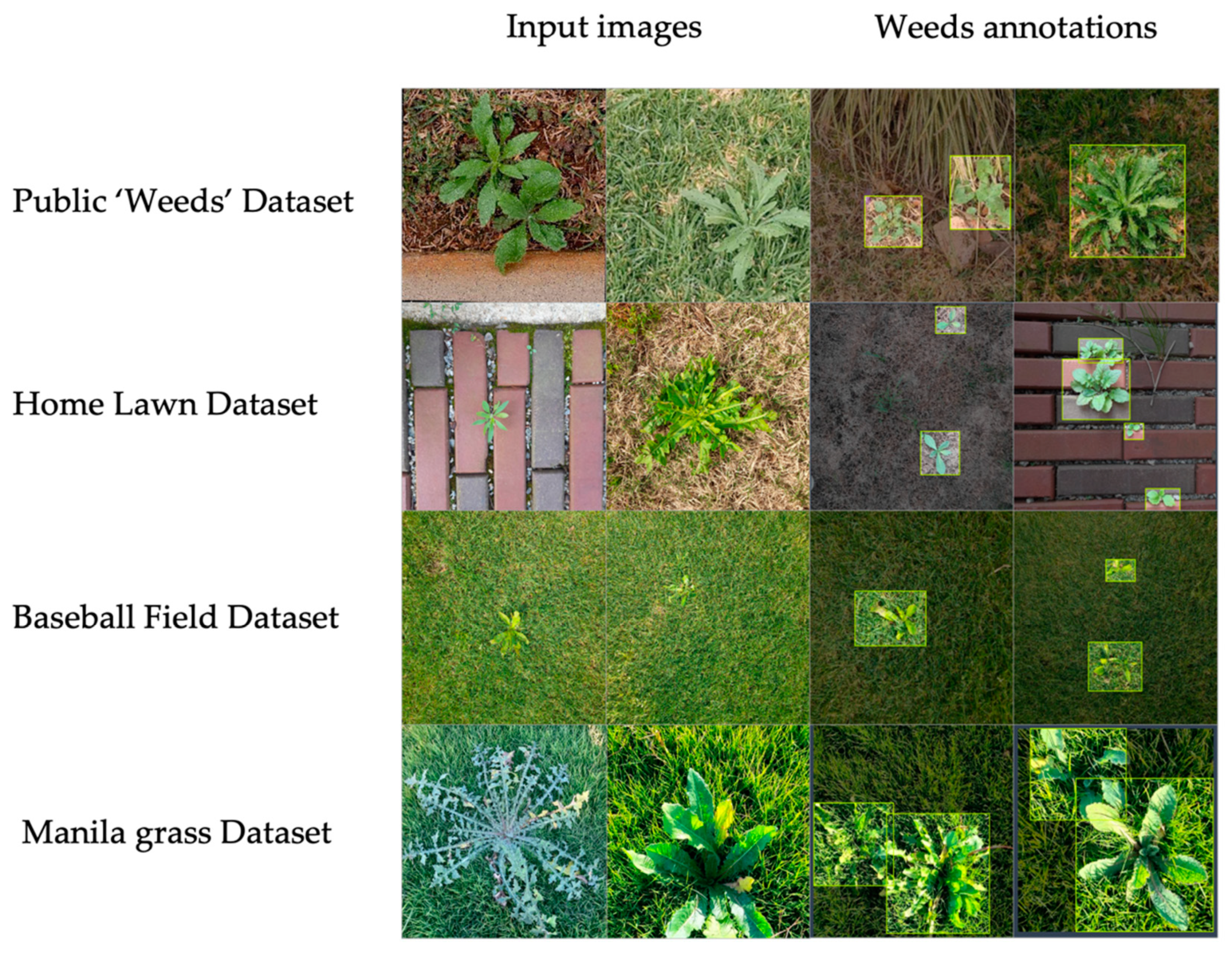
2.2. Datasets Description and Preparation

2.2.1. The ‘Weeds’ Public Dataset

A public ‘Weeds’ dataset [54] was used for this trial to train the different YOLO models. The ‘Weeds’ dataset is a collection of weeds growing in lawns and in typical urban backgrounds that can easily confuse object detection models due to the similarity of the weeds with their surroundings. This dataset contains 4203 images with weeds labeled for 11,385 annotations. The ‘Weeds’ dataset contains approximately 62% of images of weeds with turf backgrounds, 13% of images with third surfaces (different floor patterns) backgrounds, and approximately 24% of images with both backgrounds (results from image analysis on 500 images sample). Weeds identified in this dataset were Erigeron canadensis L. (43%), Sonchus spp. (23%), Taraxacum officinale L. (weber) (18%), Oxalis spp. (4%), Cerastium spp. (3%) and a small percentage of unknown (results from image analysis on 500 images sample). No sufficient images for each species were provided in the dataset for training multi-class detectors; thus, only one class (Weeds) was assumed for this trial. The labels correlogram in the relationship between the position, width, and height of the dataset’s objects (weeds) annotations. Generally, our datasets contain mostly small and stretched objects positioned at the center of the digital image. Before training the model, the images were cropped to obtain a resolution of 640 × 640 pixels without applying any resizing and were subjected to the auto-orient function. The auto-orient strips images of their EXIF data to be displayed in the same way as they are stored on disk.

To assess the model’s performance on this dataset, a k-fold cross-validation was performed. K-fold cross-validation is a simple popular method for model evaluation. This procedure generally consists of dividing the dataset into k subsets after a random shuffle, training the model on k-1 subsets, and using the remaining subset to test the model. The evaluation scores produced are considered more reliable as a model performance summary. This dataset was divided into five subsets (two of 804 and three of 805 images); therefore, a five-fold cross-validation was performed. The best-performing models of each YOLO version were then trained on the dataset (train: 3664 images, validation: 359 images, and test: 180 images) and evaluated. The online platform Google Colaboratory (Colab), offered by Google, was used to implement and train the model. Colab, a cloud service based on Jupyter Notebooks, provides a free single 12 GB NVIDIA Tesla K80 GPU.

2.2.2. Additional Test Datasets

Furthermore, three additional test datasets were used to evaluate different model detection and to assess the potential use of the trained models for weed detection in other contexts.

The Home Lawn dataset comprises 180 images featuring 473 annotations of weeds proliferating in a mature stand of bermudagrass (Cynodon dactylon (L.) Pers.) during its early green-up phase (indicative of low-quality turf) as well as weeds emerging on hard surfaces such as streets, curbs, and brick floors. These intricate background settings, commonly found in residential and urban areas, could potentially influence the efficacy of weed detection. The images were captured in various locations, including residential lawns and parks, in Seville, Spain (37°389 N, 5°985 W; Datum: WGS84).

The Baseball Field dataset comprised 180 images and 285 annotations of weeds developing in a bermudagrass turf overseeded with ryegrass (Lolium perenne L.) actively growing. In this dataset, image backgrounds are considered uniform (high-quality turf) and most weeds are small in size and partially growing within the turf or with altered shapes due to the intense management. Images of this dataset were collected at the Opelika High School baseball field (Opelika, AL, USA; 32°645 N, 85°378 W; Datum: WGS84).

The Manila grass dataset consisted of 180 digital images and 242 annotations of weeds developing in a mature stand of manila grass (Zoysia matrella (L.) Merr. cv ‘Diamond’) actively growing. In this dataset, most weeds are large in size and with full growth shape. Images were taken at the experimental farm of the Department of Agriculture, Food and Environment of the University of Pisa (San Piero a Grado, Pisa, Italy; 43°400 N, 10°190 E; Datum: WGS84).

In all datasets, T. officinale, Plantago lanceolata L., and Sonchus spp. were identified as significant weed species and examples of imags are depicted in Figure 1.

The Robotflow API (https://app.roboflow.com; accessed on 2 July 2023) was used to annotate additional test dataset images and convert them into the respective YOLO version format and dataset split for the five-fold cross-validation.

2.3. Metrics

The trained models for weed detection were tested on the test subset and three additional small datasets mentioned in Section 2.2.2. The number of weeds per image was manually counted and reported as a ground truth value. Consequently, with this data, precision (P) and recall (R) were used as the evaluation metrics for weed detection. These model evaluation metrics are defined as follows:

$$\mathrm{P}\mathrm{r}\mathrm{e}\mathrm{c}\mathrm{i}\mathrm{s}\mathrm{i}\mathrm{o}\mathrm{n}(\mathrm{P})=\frac{\mathrm{T}\mathrm{P}}{\mathrm{T}\mathrm{P}+\mathrm{F}\mathrm{P}}$$

(1)

$$\mathrm{R}\mathrm{e}\mathrm{c}\mathrm{a}\mathrm{l}\mathrm{l}\left(\mathrm{R}\right)=\frac{\mathrm{T}\mathrm{P}}{\mathrm{T}\mathrm{P}+\mathrm{F}\mathrm{N}}$$

(2)

where TP consists of the true positives (when the algorithm correctly detects weeds with a bounding box); FP corresponds to the false positives (when the algorithm computes a bounding box in a location without weeds); and FN indicates false negatives (when a target weed is not detected). The IoU between the bounding box produced by the detection and the ground truth is calculated. For each image, If the IoU is over a predetermined threshold (0.5 in this study), a TP is produced; otherwise, the result is an FP. As mentioned in Section 2.1, the trained model provides a TP using bounding box coordinates and a confidence score (the model’s confidence regarding each detection performed). The area under the precision–recall curve represents the average precision (AP).

$$\mathrm{A}\mathrm{v}\mathrm{e}\mathrm{r}\mathrm{a}\mathrm{g}\mathrm{e}\mathrm{P}\mathrm{r}\mathrm{e}\mathrm{c}\mathrm{i}\mathrm{s}\mathrm{i}\mathrm{o}\mathrm{n}\left(\mathrm{A}\mathrm{P}\right)={\int }_0^1\mathrm{P}\left(\mathrm{R}\right)\mathrm{d}\mathrm{R}$$

(3)

AP is a number between 0 and 1 used to summarize the different precision values obtained in the recall function. Furthermore, the mean average precision (mAP) is used to evaluate a model and is obtained by averaging the AP for each class.

$$\mathrm{M}\mathrm{e}\mathrm{a}\mathrm{n}\mathrm{A}\mathrm{v}\mathrm{e}\mathrm{r}\mathrm{a}\mathrm{g}\mathrm{e}\mathrm{P}\mathrm{r}\mathrm{e}\mathrm{c}\mathrm{i}\mathrm{s}\mathrm{i}\mathrm{o}\mathrm{n}\left(\mathrm{m}\mathrm{A}\mathrm{P}\right)=\frac{1}{\mathrm{n}}{\sum }_{\mathrm{i}=1}^{\mathrm{i}=\mathrm{n}}\mathrm{A}\mathrm{P}\mathrm{i}$$

(4)

Generally, two maps are produced using two different thresholds: the mAP_0.5, the mean of the AP with a confidence score between 0 and 0.5, and the mAP_0.5:0.95, which is the mean of the AP with a confidence score between 0.5 and 0.95. Therefore, precision (P), recall (R), mean average precision 0.5 (mAP_0.5), and represent average precision 0.5–0.95 (mAP_0.5:0.95) are considered the most common metrics when evaluating object detectors [25].

Models performance metrics (P, R, mAP_0.5 and mAP_0.5:0.95) obtained after the 5-fold cross validation have been subjected to a one-way ANOVA using statistical software R [55]. Data normality assumptions were assessed using the Shapiro-Wilk for normality and Levene’s test for homoscedasticity using ‘car’ package [56]. Pairwise comparisons and mean separation were performed with a Tukey HSD post hoc test (FDR adjusted p-value) using ‘scmamp’ package [57]. In Figure 2 is depicted and resumed the framework of the current study.

3. Results and Discussion

The Analysis of variance revealed significant differences on models performance metrics (

Table 3. Results on five-fold cross validation test of different models studied.

Model	Precision		Recall		mAP_0.5		mAP_0.5:0.95
EfficientDet	0.9033 ± 0.0244 *	b **	0.8862 ± 0.0312	c	0.8931 ± 0.0312	d	0.7172 ± 0.0313	ef
YOLOv5n	0.9259 ± 0.0102	ab	0.893 ± 0.0594	bc	0.9343 ± 0.0387	abcd	0.7002 ± 0.012	f
YOLOv5s	0.9445 ± 0.0281	a	0.756 ± 0.0233	de	0.9104 ± 0.0408	bcd	0.8674 ± 0.0664	a
YOLOv5m	0.9305 ± 0.0484	ab	0.7305 ± 0.0381	e	0.9057 ± 0.0307	cd	0.8841 ± 0.0795	a
YOLOv5l	0.9264 ± 0.0484	ab	0.7313 ± 0.0672	e	0.9197 ± 0.0333	abcd	0.8606 ± 0.0442	a
YOLOv5x	0.939 ± 0.0459	ab	0.7928 ± 0.0181	d	0.9104 ± 0.06	bcd	0.8789 ± 0.0507	a
YOLOv6n	0.9456 ± 0.0146	a	0.7594 ± 0.0172	de	0.9539 ± 0.0142	ab	0.7112 ± 0.0093	ef
YOLOv6s	0.9331 ± 0.0294	ab	0.7707 ± 0.0223	de	0.9392 ± 0.0286	abc	0.7208 ± 0.0186	ef
YOLOv6m	0.9401 ± 0.0237	ab	0.7344 ± 0.0293	e	0.9237 ± 0.0354	abcd	0.7156 ± 0.0192	ef
YOLOv6l	0.9414 ± 0.023	a	0.7728 ± 0.0346	de	0.9508 ± 0.0147	ab	0.7277 ± 0.0178	def
YOLOv7	0.9111 ± 0.0209	ab	0.9552 ± 0.0136	a	0.9594 ± 0.0214	a	0.7625 ± 0.014	bcde
YOLOv7x	0.9398 ± 0.0238	ab	0.9338 ± 0.0321	ab	0.9366 ± 0.0302	abcd	0.7393 ± 0.0244	cdef
YOLOv8n	0.9266 ± 0.0265	ab	0.9269 ± 0.0271	abc	0.9412 ± 0.0202	abc	0.7547 ± 0.0403	bcde
YOLOv8s	0.9169 ± 0.0275	ab	0.939 ± 0.0526	ab	0.9051 ± 0.0625	cd	0.7517 ± 0.043	bcdef
YOLOv8m	0.9227 ± 0.0257	ab	0.9247 ± 0.0363	abc	0.9385 ± 0.0326	abc	0.7769 ± 0.0302	bcd
YOLOv8l	0.9235 ± 0.0276	ab	0.9244 ± 0.0417	abc	0.955 ± 0.0263	a	0.8043 ± 0.015	b
YOLOv8x	0.9304 ± 0.021	ab	0.9189 ± 0.0417	abc	0.9477 ± 0.0296	abc	0.7925 ± 0.0333	bc

* Values refer to the mean and standard deviation of models performance on five-fold cross validation. ** Different letters on the same column represent different values at p < 0.05.

). Among these models, YOLOv5s, YOLOv6n, and YOLOv6l achieved the highest precision (P) scores with values of 0.9445 ± 0.0281, 0.9456 ± 0.0146, and 0.9414 ± 0.023, respectively. Notably, these three models exhibited significantly higher precision scores compared to EfficientDet, which yielded the lowest precision score of 0.9033 ± 0.0244 (p < 0.05). Conversely, no significant differences in precision scores were observed among the other models. Regarding the recall (R) metric, YOLOv7 yielded the best results with a score of 0.9552 ± 0.0136. No significant differences were found between YOLOv7 and YOLOv7x, as well as all scales of YOLOv8 models. However, YOLOv7 displayed significant differences when compared to EfficientDet (p < 0.01) and all scales of YOLOv5 and YOLOv6 models (p < 0.001, except for YOLOv5n with a p < 0.05). For the mean average precision at an intersection over union (IOU) threshold of 0.5 (mAP_0.5), YOLOv8 and YOLOv7 demonstrated the highest performance with scores of 0.9594 ± 0.0214 and 0.955 ± 0.0263, respectively. No significant differences were observed between these models and all scales of YOLOv6, YOLOv7x, and YOLOv8 (except for YOLOv8s with p < 0.05), as well as YOLOv5s and YOLOv5l. Conversely, all other models exhibited significantly lower mAP_0.5 values, with EfficientDet performing the worst (p < 0.01, with a score of 0.8931 ± 0.0312). In terms of the mAP_0.5 to 0.95 metric, all YOLOv5 models (except YOLOV5n with p < 0.001) achieved the best results, ranging from 0.8841 ± 0.0795 for YOLOv5m to 0.8606 ± 0.0442 for YOLOv5l. YOLOv8l exhibited a significantly lower mAP_0.5 to 0.95 score (p < 0.01) compared to other YOLOv8 models, but it was the best-performing model within the YOLOv8 series, achieving a score of 0.8043 ± 0.015. No significant differences were found between YOLOv8l and other YOLOv8 models, as well as YOLOv7. Notably, all other models displayed significantly lower mAP_0.5 to 0.95 scores, with YOLOv5n performing the worst (p < 0.001) at a value of 0.7002 ± 0.012.

According to results from the five-fold cross-validation experiment, ten models (YOLOv5n, YOLOv5s, YOLOv5m, YOLOv6n, YOLOv6l, YOLOv7, YOLOv7x, YOLOv8s, YOLOv8l, and YOLOv8x) were trained on the ‘Weeds’ public dataset for 100 epochs (Table 2) and best performing models for each YOLO version were selected to be tested on the four different test datasets. Performances of the ten models are resumed and depicted in Figure 3.

In general, YOLOv6 model scales depicted a different trend during the train process since this model provide evaluation at the first epoch, the 20th, the 40th, and every three epochs starting from the 50th. Among YOLOv5 model scales, YOLOv5s obtained the highest P (0.9485), while YOLOv5m obtained the best R (0.9761), mAP_0.5 (0.9783) and mAP0.5:0.95 (0.7811). Among the YOLOv6 models, YOLOv6n obtained the best P (0.9646) and best mAP_0.5 (0.9651), while YOLOv6l resulted with the best R (0.8893) and best mAP_0.5:0.95 (0.7421). YOLOv7 surpassed YOLOv7x for all the metrics resulting in P (0.9466), R (0.9663), mAP_0.5 (0.9758), and mAP_0.5:0.95 (0.7672). Among YOLOv8 model scales, YOLOv8x obtained the best P and R values (0.95463 and 0.9761, respectively) while YOLOv8l resulted with the best mAP_0.5 and mAP_0.5:0.95 (0.9775 and 0.8129, respectively). Based on these results, YOLOv5m, YOLOv6l, YOLOv7, and YOLOv8l were tested on the four different test datasets. The results of this trial are reported in

Table 4. Performance and inference time of best YOLO model scales for the four studied YOLO versions (YOLOv5m, YOLOv6l, YOLOv7, and YOLOv8l) and EfficientDet.

Model	Dataset	P	R	mAP_0.5	mAP_0.5:0.95	Inference (ms) a
EfficientDet	‘Weeds’ public	0.9133	0.9273	0.9426	0.7023	44.3
	Home Lawn	0.5982	0.5149	0.5195	0.4155	52.0
	Baseball Field	0.6138	0.7069	0.6614	0.4136	54.2
	Manila grass	0.6047	0.6954	0.5691	0.4369	50.1
YOLOv5m	‘Weeds’ public	0.9433	0.9663	0.9772	0.7828	16.2
	Home Lawn	0.6331	0.5272	0.5399	0.4263	19.2
	Baseball Field	0.6856	0.8126	0.7135	0.4716	24.1
	Manila grass	0.6441	0.5433	0.6412	0.5007	18.7
YOLOv6l	‘Weeds’ public	0.9442	0.9494	0.9747	0.7612	22.8
	Home Lawn	0.7836	0.6446	0.7057	0.5022	32.5
	Baseball Field	0.6098	0.6491	0.5379	0.4108	47.9
	Manila grass	0.5865	0.7571	0.7014	0.5248	26.6
YOLOv7	‘Weeds’ public	0.9265	0.9627	0.9745	0.7685	16.1
	Home Lawn	0.7118	0.6454	0.7108	0.5209	29.1
	Baseball Field	0.6223	0.7579	0.6379	0.4009	35.6
	Manila grass	0.6549	0.7571	0.6461	0.4614	27.5
YOLOv8l	‘Weeds’ public	0.9476	0.9610	0.9795	0.8123	34.0
	Home Lawn	0.6567	0.6422	0.6564	0.4721	37.4
	Baseball Field	0.6672	0.6474	0.6459	0.4312	19.7
	Manila grass	0.7635	0.6519	0.7589	0.5296	36.6

^a Inference time refers to the average time needed for the model to detect weeds on a single digital image.

.

Table 4 shows the results of the YOLO model’s detection on the four test datasets (confusion matrix is reported in

Table A1. Confusion matrices of studied models.

Model	Dataset	TP	FP	FN	TN
EfficientDet	‘Weeds’ public	412	39	46	0
	Home Lawn	164	117	161	0
	Baseball Field	154	95	63	0
	Manila grass	95	61	41	0
YOLOv5m	‘Weeds’ public	492	31	26	0
	Home Lawn	222	127	199	0
	Baseball Field	139	63	56	0
	Manila grass	103	56	89	0
YOLOv6l	‘Weeds’ public	478	28	31	0
	Home Lawn	226	63	126	0
	Baseball Field	187	81	72	0
	Manila grass	138	101	49	0
YOLOv7	‘Weeds’ public	482	39	18	0
	Home Lawn	250	101	136	0
	Baseball Field	175	106	58	0
	Manila grass	191	101	58	0
YOLOv8l	‘Weeds’ public	499	31	23	0
	Home Lawn	243	132	138	0
	Baseball Field	198	101	114	0
	Manila grass	178	55	99	0

of Appendix A). All the tested models obtained higher performances on the ‘Weeds’ public dataset than the additional test datasets. For this test, YOLOv8l resulted with the highest P value (0.9476), best mAP_0.5 (0.9795), and mAP_0.5:0.95 (0.8123). YOLOv5m resulted in the highest R (0.9663). The time required for models to inference on this test dataset was approximately 34 ms per image for YOLOv8l and 16.2 ms for YOLOv5m. When performing inference on the Home Lawn dataset, YOLOv6l resulted with the best P (0.7836), while YOLOv7 obtained the best R (0.6454), best mAP_0.5 (0.7108), best mAP_0.5:0.95 (0.5209). The inference time required for this dataset was approximately 32.5 ms for YOLOv6l and 29.1 ms for YOLOv7. The best models performing inference on the Baseball Field dataset were YOLOv5m with the best P (0.6856), best R (0.8126), mAP_0.5 (0.7135) and best mAP_0.5:0.95 (0.4716). The inference time required was approximately 24.1 ms for YOLOv5m. For the Manila grass dataset, the best P was obtained from YOLOv8l (0.7635), and the best R was obtained from YOLOv7 and YOLOv6l (both models got R of 0.7571). YOLOv8l resulted in the highest mAP_0.5 and mAP_0.5:0.95 (0.7589 and 0.5296, respectively). Yu et al. [18] trained and tested multiple species of two-stage detectors to detect different weeds among actively growing perennial ryegrass, obtaining higher values of R (>0.98). Low R values suggest that the model misclassifies target weeds as turfgrass, thus producing an FN. This is unacceptable for field applications since weeds would be missed, leading to unsatisfactory weed control in turfgrass. Figure 4 shows an example of YOLOv5m, YOLOv6l, YOLOv7, and YOLOv8l weeds detection on the test datasets.

As shown in Figure 4, the model effectively detected weeds at a mature stage (>5 true leaves) growing outside from a turfgrass canopy. The training dataset consists of a multiple weed species dataset, most of which were rosettae-forming weeds grow in turfgrasses. For this reason, the model showed high performances in a situation similar to those occurring in the public ‘Weeds’ dataset. These findings are in accordance with [20]. In this research, authors argued that the detection is highly affected by the broad-leaved weeds morphology and leaf pattern and color variations among species and within the same species. The authors proposed that multiple-species neural network training and images gathered from different geographical regions (to include various turf sites and weed biotypes) may be beneficial for the overall accuracy of weed detection models. However, the results obtained from experiments conducted on different datasets suggest that efforts are still required to improve the overall accuracy. Benjumea et al. [58] proposed an improved YOLO architecture that allows a more efficient detection of smaller objects. A more minor object detection was improved by modifying the architecture structure and fine-tuning parameters and resulted in an increased mAP_0.5 of approximately 7% without significantly affecting the inference time. Moreover, the models failed to detect weeds close to the image edge. Yu et al. [19] claim that the edge effect may be reduced by the continuous frames inputs (since in field applications, weed detection is based on videos), thus boosting detection accuracy. In this trial, all the models were able to detect weeds at the edge of the image frames. Furthermore, highly complex backgrounds such as low-quality turf may increase the computational complexity for feature extraction and a reduced R of the model [19]. In this trial, only YOLOv5m models agree with this finding. Indeed, YOLOv5m obtained the lowest R when detecting weeds in the Home Lawn dataset, which had the most complex background. This limitation may be overcome by increasing the number of training images. Zhuang et al. [28] obtained similar low P and R values when using YOLOv3 for R. scabra detection in drought-stressed and unstressed turfgrasses. In this research, authors argued that high background variability in the training dataset increases cause a less efficient feature extraction and consequently decreases P and R metrics. For this reason, the authors suggest further research on training object detectors on images with the simplest background. Additionally, the annotation method used in this trial consisted of drawing bounding boxes around the weed within the image, which is not the method with the highest resolution. Indeed, Sharpe et al. [59] demonstrate that higher-resolution annotation methods improve the overall neural network accuracy. Moreover, artificial neural networks recognize plants using color, texture, and shape features [60], and Hahn et al. [61] found that multispectral components are highly effective in broadleaves weed detection in turfgrass. Thus, further research may be addressed to assess and clarify how these techniques and methods can improve detector’s performances. According to Yang et al. [62], high image processing speed is imperative for real-time weed detection and treatment. Eventual actuators for weed control would only have a few seconds to detect weeds by processing images and delivering the treatments.

The obtained results revealed disparities in the required inference time among different models. Specifically, YOLOv5m exhibited efficient inference time, taking less than 20 ms for all the datasets except for the Baseball Field, where it required approximately 24 ms. Similarly, YOLOv6l and YOLOv7 showed a similar trend, achieving detection within less than 30 ms for the public ‘Weeds’, Home Lawn and Manila grass datasets, while requiring longer inference time for the Baseball Filed dataset. For YOLOv5m, YOLOv6l and YOLOv7, the average mAP_0.5 values were 0.72, 0,73 and 0.74, respectively, with corresponding average mAP_0.5:0.95 values of 0.55, 0.55 and 0.54. Notably, YOLOv5m and YOLOv7 consistently achieved detections in less than 30 ms, while YOLOv6l resulted with an average inference time of 33 ms (Figure 5). Conversely, YOLOv8l exhibited a contrasting trend, requiring more than 30 ms for inference on all test datasets, except for the Baseball Field dataset, where it required less than 20 ms. YOLOv8l resulted with an average mAP_0.5 of 0.76 and an average mAP_0.5:0.95 of 0.56, with an average inference time of 32 ms. On the other hand, EfficientDet exhibited the lowest average mAP_0.5 and mAP_0.5:0.95 (0.67 and 0.49, respectively) and the highest average inference time (50 ms). The situation among inference time, models and test datasets is not straightforward and warrants further investigation for clarification. Thus, additional studies should be conducted to explore and elucidate the intricate dynamics among these factors.

4. Conclusions

The task of achieving satisfactory weed detection in turfgrass through training digital images poses significant challenges. In this study, different YOLO object detectors were prepared and tested for weed detection in turfgrasses, considering different weeds species as a single class (‘Weeds’). Among the tested models, YOLOv8l demonstrated the highest overall performance on the test dataset, achieving a precision of 0.9476, mAP_0.5 of 0.9795, and mAP_0.5:0.95 of 0.8123. Despite YOLOv8l high performances, results on the additional test datasets were not acceptable for a professional use. Consequently, it became evident that several obstacles hinder accurate weed detection, emphasizing the need for more in-depth research. To enhance performance, future investigations should focus on exploring weed detection algorithms that incorporate multiple vegetative indices and features. Additionally, alternative annotation techniques, such as instance segmentation, should be compared with the more conventional bounding box-based object detection to determine whether different techniques can potentially yield improvements in weed identification. Moreover, a broad spectrum of weed species and ecotypes should be included in the training and testing of weed detection algorithms to ensure accurate performance in turfgrass scenarios. In conclusion, the findings of this study underscore the challenges associated with weed detection in turfgrass using digital image training. Further research endeavors are imperative to address the identified limitations and advance the field of weed detection in turfgrass through the exploration of enhanced algorithms, annotation techniques, and broader inclusion of weed species and ecotypes.

References

1. McElroy, J.S.; Martins, D. Use of Herbicides on Turfgrass. Planta Daninha 2013, 31, 455–467. [Google Scholar] [CrossRef] [Green Version]
2. Karabelas, A.J.; Plakas, K.V.; Solomou, E.S.; Drossou, V.; Sarigiannis, D.A. Impact of European Legislation on Marketed Pesticides—A View from the Standpoint of Health Impact Assessment Studies. Environ. Int. 2009, 35, 1096–1107. [Google Scholar] [CrossRef]
3. Stoate, C.; Báldi, A.; Beja, P.; Boatman, N.D.; Herzon, I.; van Doorn, A.; de Snoo, G.R.; Rakosy, L.; Ramwell, C. Ecological Impacts of Early 21st Century Agricultural Change in Europe—A Review. J. Environ. Manag. 2009, 91, 22–46. [Google Scholar] [CrossRef]
4. European Commission. EU Pesticides Database 2022. Available online: https://food.ec.europa.eu/plants/pesticides/eu-pesticides-database_en (accessed on 2 July 2023).
5. Hahn, D.; Sallenave, R.; Pornaro, C.; Leinauer, B. Managing Cool-Season Turfgrass without Herbicides: Optimizing Maintenance Practices to Control Weeds. Crop Sci. 2020, 60, 2204–2220. [Google Scholar] [CrossRef] [Green Version]
6. Martelloni, L.; Frasconi, C.; Sportelli, M.; Fontanelli, M.; Raffaelli, M.; Peruzzi, A. Flaming, Glyphosate, Hot Foam and Nonanoic Acid for Weed Control: A Comparison. Agronomy 2020, 10, 129. [Google Scholar] [CrossRef] [Green Version]
7. Jin, X.; McCullough, P.E.; Liu, T.; Yang, D.; Zhu, W.; Chen, Y.; Yu, J. A Smart Sprayer for Weed Control in Bermudagrass Turf Based on the Herbicide Weed Control Spectrum. Crop Prot. 2023, 170, 106270. [Google Scholar] [CrossRef]
8. Jin, X.; Bagavathiannan, M.; Maity, A.; Chen, Y.; Yu, J. Deep Learning for Detecting Herbicide Weed Control Spectrum in Turfgrass. Plant Methods 2022, 18, 94. [Google Scholar] [CrossRef]
9. Jin, X.; Liu, T.; McCullough, P.E.; Chen, Y.; Yu, J. Evaluation of Convolutional Neural Networks for Herbicide Susceptibility-Based Weed Detection in Turf. Front. Plant Sci. 2023, 14, 1096802. [Google Scholar] [CrossRef]
10. Watchareeruetai, U.; Takeuchi, Y.; Matsumoto, T.; Kudo, H.; Ohnishi, N. Computer Vision Based Methods for Detecting Weeds in Lawns. In Proceedings of the 2006 IEEE Conference on Cybernetics and Intelligent Systems, Bangkok, Thailand, 7–9 June 2006; Volume 1. [Google Scholar] [CrossRef]
11. Weis, M.; Rumpf, T.; Gerhards, R.; Plümer, L. Comparison of Different Classification Algorithms for Weed Detection from Images Based on Shape Parameters. Bornimer Agrar. Ber. 2009, 69, 53–64. [Google Scholar]
12. Gebhardt, S.; Schellberg, J.; Lock, R.; Kühbauch, W. Identification of Broad-Leaved Dock (Rumex obtusifolius L.) on Grassland by Means of Digital Image Processing. Precis. Agric. 2006, 7, 165–178. [Google Scholar] [CrossRef]
13. Gebhardt, S.; Kühbauch, W. A New Algorithm for Automatic Rumex Obtusifolius Detection in Digital Images Using Colour and Texture Features and the Influence of Image Resolution. Precis. Agric. 2007, 8, 1–13. [Google Scholar] [CrossRef]
14. Parra, L.; Marin, J.; Yousfi, S.; Rincón, G.; Mauri, P.V.; Lloret, J. Edge Detection for Weed Recognition in Lawns. Comput. Electron. Agric. 2020, 176, 105684. [Google Scholar] [CrossRef]
15. Gu, J.; Wang, Z.; Kuen, J.; Ma, L.; Shahroudy, A.; Shuai, B.; Liu, T.; Wang, X.; Wang, G.; Cai, J.; et al. Recent Advances in Convolutional Neural Networks. Pattern Recognit. 2018, 77, 354–377. [Google Scholar] [CrossRef] [Green Version]
16. Lecun, Y.; Bengio, Y.; Hinton, G. Deep Learning. Nature 2015, 521, 436–444. [Google Scholar] [CrossRef] [PubMed]
17. Coleman, G.R.Y.; Bender, A.; Hu, K.; Sharpe, S.M.; Schumann, A.W.; Wang, Z.; Bagavathiannan, M.V.; Boyd, N.S.; Walsh, M.J. Weed Detection to Weed Recognition: Reviewing 50 Years of Research to Identify Constraints and Opportunities for Large-Scale Cropping Systems. Weed Technol. 2022, 36, 741–757. [Google Scholar] [CrossRef]
18. Yu, J.; Sharpe, S.M.; Schumann, A.W.; Boyd, N.S. Deep Learning for Image-Based Weed Detection in Turfgrass. Eur. J. Agron. 2019, 104, 78–84. [Google Scholar] [CrossRef]
19. Yu, J.; Sharpe, S.M.; Schumann, A.W.; Boyd, N.S. Detection of Broadleaf Weeds Growing in Turfgrass with Convolutional Neural Networks. Pest Manag. Sci. 2019, 75, 2211–2218. [Google Scholar] [CrossRef]
20. Yu, J.; Schumann, A.W.; Cao, Z.; Sharpe, S.M.; Boyd, N.S. Weed Detection in Perennial Ryegrass with Deep Learning Convolutional Neural Network. Front. Plant Sci. 2019, 10, 1422. [Google Scholar] [CrossRef] [PubMed] [Green Version]
21. Jin, X.; Bagavathiannan, M.; McCullough, P.E.; Chen, Y.; Yu, J. A Deep Learning-Based Method for Classification, Detection, and Localization of Weeds in Turfgrass. Pest Manag. Sci. 2022, 78, 4809–4821. [Google Scholar] [CrossRef]
22. Redmon, J.; Divvala, S.; Girshick, R.; Farhadi, A. You Only Look Once: Unified, Real-Time Object Detection. In Proceedings of the 2016 IEEE Conference on Computer Vision and Pattern Recognition (CVPR), Las Vegas, NV, USA, 27–30 June 2016; pp. 779–788. [Google Scholar] [CrossRef] [Green Version]
23. Everingham, M.; Eslami, S.M.A.; Van Gool, L.; Williams, C.K.I.; Winn, J.; Zisserman, A. The Pascal Visual Object Classes Challenge: A Retrospective. Int. J. Comput. Vis. 2015, 111, 98–136. [Google Scholar] [CrossRef]
24. Lin, T.-Y.; Maire, M.; Belongie, S.; Hays, J.; Perona, P.; Ramanan, D.; Dollár, P.; Zitnick, C.L. Microsoft COCO: Common Objects in Context BT—Computer Vision—ECCV 2014; Fleet, D., Pajdla, T., Schiele, B., Tuytelaars, T., Eds.; Springer International Publishing: Cham, Germany, 2014; pp. 740–755. [Google Scholar]
25. Dang, F.; Chen, D.; Lu, Y.; Li, Z. Yoloweeds: A Novel Benchmark of Yolo Object Detectors for Multi-Class Weed Detection in Cotton Production Systems. Comput. Electron. Agric. 2023, 205, 107655. [Google Scholar] [CrossRef]
26. Ying, B.; Xu, Y.; Zhang, S.; Shi, Y.; Liu, L. Traitement Du Signal Weed Detection in Images of Carrot Fields Based on Improved YOLO V4. Trait. Du Signal 2021, 38, 341–348. [Google Scholar] [CrossRef]
27. Chen, J.; Wang, H.; Zhang, H.; Luo, T.; Wei, D.; Long, T.; Wang, Z. Weed Detection in Sesame Fields Using a YOLO Model with an Enhanced Attention Mechanism and Feature Fusion. Comput. Electron. Agric. 2022, 202, 107412. [Google Scholar] [CrossRef]
28. Zhuang, J.; Jin, X.; Chen, Y.; Meng, W.; Wang, Y.; Yu, J.; Muthukumar, B. Drought Stress Impact on the Performance of Deep Convolutional Neural Networks for Weed Detection in Bahiagrass. Grass Forage Sci. 2023, 78, 214–223. [Google Scholar] [CrossRef]
29. Medrano, R. Feasibility of Real-Time Weed Detection in Turfgrass on an Edge Device. Master’s Thesis, California State Univeristy, Camarillo, CA, USA, 2021. [Google Scholar]
30. Redmon, J.; Farhadi, A. YOLO9000: Better, Faster, Stronger. In Proceedings of the 30th IEEE Conference on Computer Vision and Pattern Recognition, Honolulu, HI, USA, 21–26 July 2017; pp. 6517–6525. [Google Scholar] [CrossRef] [Green Version]
31. Redmon, J.; Farhadi, A. YOLOv3: An Incremental Improvement. arXiv 2018, arXiv:1804.02767. [Google Scholar]
32. Bochkovskiy, A.; Wang, C.-Y.; Liao, H.-Y.M. YOLOv4: Optimal Speed and Accuracy of Object Detection. arXiv 2020, arXiv:2004.10934. [Google Scholar]
33. Jocher, G. Ultralytics/Yolov5: v3.1—Bug Fixes and Performance Improvements. Zenodo 2020. Available online: https://zenodo.org/record/4154370 (accessed on 2 July 2023).
34. Li, C.; Li, L.; Geng, Y.; Jiang, H.; Cheng, M.; Zhang, B.; Ke, Z.; Xu, X.; Chu, X. YOLOv6 v3.0: A Full-Scale Reloading. arXiv 2023, arXiv:2301.05586. [Google Scholar]
35. Wang, C.-Y.; Bochkovskiy, A.; Liao, H.-Y.M. YOLOv7: Trainable Bag-of-Freebies Sets New State-of-the-Art for Real-Time Object Detectors. In Proceedings of the IEEE/CVF Conference on Computer Vision and Pattern Recognition, New Orleans, LA, USA, 18–24 June 2022; pp. 1571–1580. [Google Scholar]
36. Ultralytics Yolov8 2023. Available online: https://github.com/ultralytics/ultralytics (accessed on 2 July 2023).
37. Wang, C.Y.; Mark Liao, H.Y.; Wu, Y.H.; Chen, P.Y.; Hsieh, J.W.; Yeh, I.H. CSPNet: A New Backbone That Can Enhance Learning Capability of CNN. In Proceedings of the 2020 IEEE/CVF Conference on Computer Vision and Pattern Recognition Workshops (CVPRW), Seattle, WA, USA, 14–19 June 2020; pp. 1571–1580. [Google Scholar] [CrossRef]
38. Wang, K.; Liew, J.H.; Zou, Y.; Zhou, D.; Feng, J. PANet: Few-Shot Image Semantic Segmentation with Prototype Alignment. In Proceedings of the 2019 IEEE/CVF International Conference on Computer Vision (ICCV), Seoul, Republic of Korea, 27 October–2 November 2019; pp. 9196–9205. [Google Scholar] [CrossRef] [Green Version]
39. Nepal, U.; Eslamiat, H. Comparing YOLOv3, YOLOv4 and YOLOv5 for Autonomous Landing Spot Detection in Faulty UAVs. Sensors 2022, 22, 464. [Google Scholar] [CrossRef]
40. Xu, R.; Lin, H.; Lu, K.; Cao, L.; Liu, Y. A Forest Fire Detection System Based on Ensemble Learning. Forests 2021, 12, 217. [Google Scholar] [CrossRef]
41. Ding, X.; Zhang, X.; Han, J.; Ding, G.; Sun, J. RepVGG: Making VGG-Style ConvNets Great Again. In Proceedings of the IEEE/CVF Conference on Computer Vision and Pattern Recognition, Long Beach, CA, USA, 15–20 June 2019. [Google Scholar]
42. Liu, S. Path Aggregation Network for Instance Segmentation. In Proceedings of the 2018 IEEE/CVF Conference on Computer Vision and Pattern Recognition (CVPR), Salt Lake City, UT, USA, 18–23 June 2018. [Google Scholar]
43. Scott, M.R. TOOD: Task-Aligned One-Stage Object Detection. In Proceedings of the 2021 IEEE/CVF International Conference on Computer Vision (ICCV), Montreal, BC, Canada, 11–17 October 2021. [Google Scholar]
44. Zhang, H.; Wang, Y.; Dayoub, F.; Niko, S. VarifocalNet: An IoU-Aware Dense Object Detector. In Proceedings of the IEEE/CVF Conference on Computer Vision and Pattern Recognition, New Orleans, LA, USA, 18–24 June 2022; pp. 8514–8523. [Google Scholar]
45. Loss, S.; Powerful, M.; For, L.; Box, B. 1 SIoU Loss: More Powerful Learning for Bounding Box Regression Zhora Gevorgyan. arXiv 2022, arXiv:2205.12740. [Google Scholar]
46. Rezatofighi, H.; Tsoi, N.; Gwak, J.; Sadeghian, A.; Reid, I.; Savarese, S. Generalized Intersection over Union: A Metric and A Loss for Bounding Box Regression. arXiv 2019, arXiv:1902.09630v2. [Google Scholar]
47. Ding, X.; Chen, H.; Zhang, X.; Huang, K.; Han, J.; Ding, G. Re-Parameterizingyouroptimizersratherthan Architectures. arXiv 2023, arXiv:2205.15242. [Google Scholar]
48. Changyong, S.; Yifan, L.; Jianfei, G.; Zheng, Y.; Chunhua, S. Channel-Wise Knowledge Distillation for Dense Prediction. In Proceedings of the IEEE/CVFInternationalConferenceonComputerVision, Montreal, BC, Canada, 11–17 October 2021; pp. 5311–5320. [Google Scholar]
49. Terven, J.; Cordova-Esparza, D. A Comprehensive Review of YOLO: From YOLOv1 to YOLOv8 and Beyond. arXiv 2023, arXiv:2304.00501. [Google Scholar]
50. Wang, C.; Liao, H.M.; Yeh, I.; Corporation, E.M. Designing Network Design Strategies Through Gradient Path Analysis. arXiv 2014, arXiv:2211.04800. [Google Scholar]
51. Wang, C.; Yeh, I.; Liao, H.M. You Only Learn One Representation: Unified Network for Multiple Tasks. arXiv 2021, arXiv:2105.04206. [Google Scholar]
52. Tan, M.; Pang, R.; Le, Q.V. EfficientDet: Scalable and Efficient Object Detection. In Proceedings of the IEEE/CVF Conference on Computer Vision and Pattern Recognition, Seattle, WA, USA, 13–19 June 2020; pp. 10778–10787. [Google Scholar] [CrossRef]
53. Tan, M.; Le, Q.V. EfficientNet: Rethinking Model Scaling for Convolutional Neural Networks. In Proceedings of the International Conference on Machine Learning, Honolulu, HI, USA, 10–15 June 2019. [Google Scholar]
54. Agumented Startups. Weeds Dataset 2021. Available online: https://universe.roboflow.com/augmented-startups/weeds-nxe1w (accessed on 2 July 2023).
55. R Core Team. Team R: A Language and Environment for Statistical Computing; Team R: Vienna, Austria, 2016. [Google Scholar]
56. Weisberg, S.; Fox, J. An R Companion to Applied Regression; Sage Publications: Thousand Oaks, CA, USA, 2011; ISBN 9781412975148. [Google Scholar]
57. Calvo, B.; Santafé, G. Scmamp: Statistical Comparison of Multiple Algorithms in Multiple Problems. R J. 2016, 8, 248–256. [Google Scholar] [CrossRef] [Green Version]
58. Benjumea, A.; Teeti, I.; Cuzzolin, F.; Bradley, A. YOLO-Z: Improving Small Object Detection in YOLOv5 for Autonomous Vehicles. arXiv 2021, arXiv:2112.11798. [Google Scholar]
59. Sharpe, S.M.; Schumann, A.W.; Boyd, N.S. Goosegrass Detection in Strawberry and Tomato Using a Convolutional Neural Network. Sci. Rep. 2020, 10, 9548. [Google Scholar] [CrossRef]
60. Qingfeng, W.; Kun-hui, L.; Chang-le, Z. Feature Extraction and Automatic Recognition of Plant Leaf Using Artificial Neural Network. Res. Comput. Sci. 2007, 20, 3–10. [Google Scholar]
61. Hahn, D.S.; Roosjen, P.; Morales, A.; Nijp, J.; Beck, L.; Velasco Cruz, C.; Leinauer, B. Detection and Quantification of Broadleaf Weeds in Turfgrass Using Close-Range Multispectral Imagery with Pixel- and Object-Based Classification. Int. J. Remote Sens. 2021, 42, 8035–8055. [Google Scholar] [CrossRef]
62. Yang, C.C.; Prasher, S.O.; Landry, J.A.; Ramaswamy, H.S.; DiTommaso, A. Application of Artificial Neural Networks in Image Recognition and Classification of Crop and Weeds. Can. Agric. Eng. 2000, 42, 147–152. [Google Scholar]
Figure 1. Weeds images and annotations randomly retrieved from the ‘Weeds’ public dataset and the three additional test datasets (Home Lawn, Baseball Field, and Manila grass).
Applsci 13 08502 g001
Figure 2. Trial framework for models’ train and evaluation on different turfgrass scenario.
Applsci 13 08502 g002
Figure 3. Results of precision (P), recall (R), mean average precision at 0.5 confidence levels (mAP_0.5), and mean average precision at 0.5–0.95 confidence levels (mAP_0.5–0.95) of best YOLO model scales for the four studied YOLO versions trained on the ‘Weeds’ public dataset for 100 epochs. (a) Different model scales Precision values for 100 epochs; (b) Different model scales Recall values for 100 epochs; (c) Different model scales mAP_0.5 values for 100 epochs; (d) Different model scales mAP_0.5:0.95 values for 100 epochs.
Applsci 13 08502 g003
Figure 4. Example of weed detections using the EfficientDet, YOLOv5m, YOLOv6l, YOLOv7, and YOLOv8l models on the four test datasets (public ‘Weeds,’ Home lawn, Baseball Field, and Manila grass).
Applsci 13 08502 g004
Figure 5. YOLO models and EfficientDet mean average precision (mAP) and inference time trade-off. Data were averaged among the four test datasets.
Applsci 13 08502 g005