Article

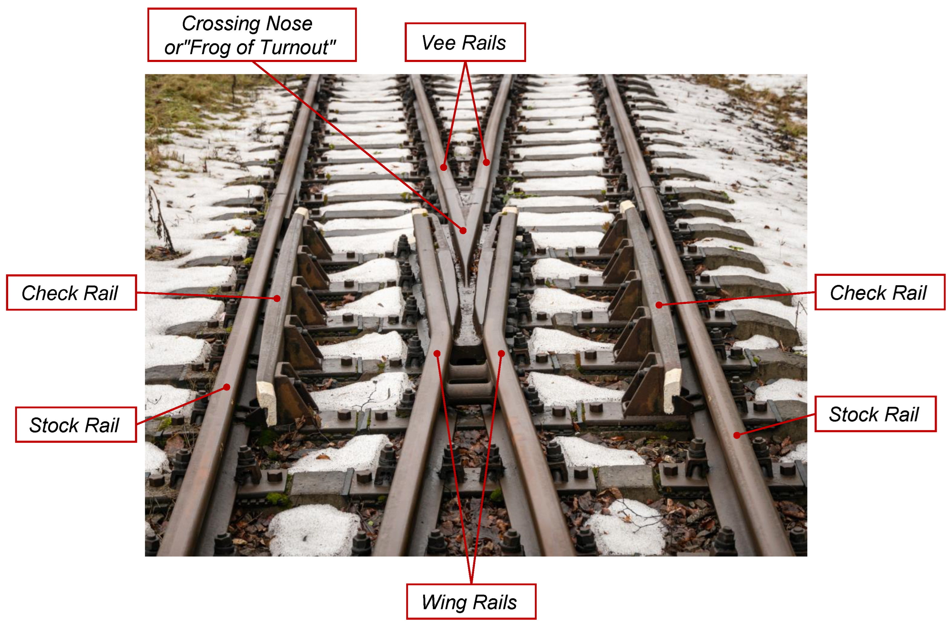
Cyclic Hardening and Fatigue Damage Features of 51CrV4 Steel for the Crossing Nose Design

by
Vítor M. G. Gomes
1,†,
Sven Eck
2,† and
Abílio M. P. De Jesus
1,*,†
1
FEUP Faculty of Engineering, University of Porto, 4200-465 Porto, Portugal
2
MCL, Materials Center Leoben Forschung GmbH, 8700 Leoben, Austria
*
Author to whom correspondence should be addressed.
These authors contributed equally to this work.
Appl. Sci. 2023, 13(14), 8308; https://doi.org/10.3390/app13148308
Submission received: 6 July 2023 / Revised: 12 July 2023 / Accepted: 14 July 2023 / Published: 18 July 2023

Abstract

:
A crossing nose is a component of railway infrastructure subject to very severe loading conditions. Depending on the severity of these loads, the occurrence of structural fatigue, severe plastic deformation, or rolling fatigue may occur. Under fatigue conditions with high plastic deformation, cyclic plasticity approaches, together with local plasticity models, become more viable for mechanical design. In this work, the fatigue behavior in strain-controlled conditions of 51CrV4 steel, applicable to the crossing nose component, was evaluated. In this investigation, both strain-life and energy-life approaches were considered for fatigue prediction analysis. The results were considered through obtaining a Ramberg-Osgood cyclic elasto-plastic curve. Since this component is subject to cyclic loading, even if spaced in time, the isotropic and kinematic cyclic hardening behavior of the Chaboche model was subsequently analyzed, considering a comparative approach between experimental data and the FEM. As a result, the material properties and finite element model parameters presented in this work can contribute to the enrichment of the literature on strain-life fatigue and cyclic plasticity, and they could be applied in mechanical designs with 51CrV4 steel components or used in other future analyses.

1. Introduction

The development of a product or machine’s component requires an adequate design for its operating conditions. In the railway sector, more specifically in railway infrastructure, different configurations of turnouts have been developed over the years, to optimize performance. A turnout, as illustrated in Figure 1, is a system that allows changing railway tracks and is one of the weak points in railway structures, in addition to small radius curves and railway joints. In the composition of a turnout, there is a component called a crossing or frog that consists of two wing rails, two V rails, and the nose of the crossing, as illustrated in Figure 1. This component is at the intersection point of the straight lane and the branched lane [1].
The investigations carried out on this component focus on structural and geometric aspects. On the one hand, the crossing geometry is designed to allow a smoother transition between lines. On the other hand, from a structural point of view, concerns are mostly associated with surface wear, structural fatigue [1], and rolling contact fatigue [2], in addition to severe plastic deformation [3]. These issues come from high-frequency use, due to high traffic levels and high magnitude contact forces from the wheel–rail interaction, which can reach higher values of about two to four times the static wheel force. Experimental and numerical investigations have been carried out, in order to identify the main features for improving the prediction of these failure phenomena. Implementation studies with digital twin techniques have been carried out, to assess the damage from fatigue [1,4,5,6].
Concerns exist regarding the dynamics between a wheel and the rail contact forces. The assessed large contact forces [1] could cause severe damage at the crossing nose, such as spalling, head checks, squashing, and cracks. Different types of steels have been used for the production of the frog of the turnout, ranging from low-alloyed constructional steel to high-alloyed quenched and tempered steel. A comparative study of the properties of different steel grades for manufacturing a crossing nose is presented in [5]. Chromium-vanadium alloyed steels have both high mechanical strength and corrosion resistance, due to the presence of chromium. The chromium-vanadium alloyed steel grade 51CrV4 (EN 1.8159) is generally quenched and tempered to obtain a good ratio of strength and ductility and resistance to fatigue [7,8,9]. Additionally, the 51CrV4 steel grade has had other engineering applications, such as in train suspension spring components [10,11,12], gears, pinions, forged crankshafts, steering knuckles, connecting rods, spindles, pumps, and gear shafts [9,13,14].
Given the highlighted concerns regarding the reliability and safety of the structural design of crossing noses, an analysis of the fatigue behavior of the 51CrV4 steel is conducted in the present paper. Furthermore, as it is a component frequently subjected to cyclic loads with high contact loads, an elasto-plastic analysis of the material was performed. Based on the data obtained from the cyclic tests, an elasto-plastic curve is suggested for the stabilized cyclic model. Additionally, the transient cyclic behavior of the material is investigated. Regarding this aspect, parameters for isotropic and kinematic hardening are suggested.

2. Fatigue Life Prediction

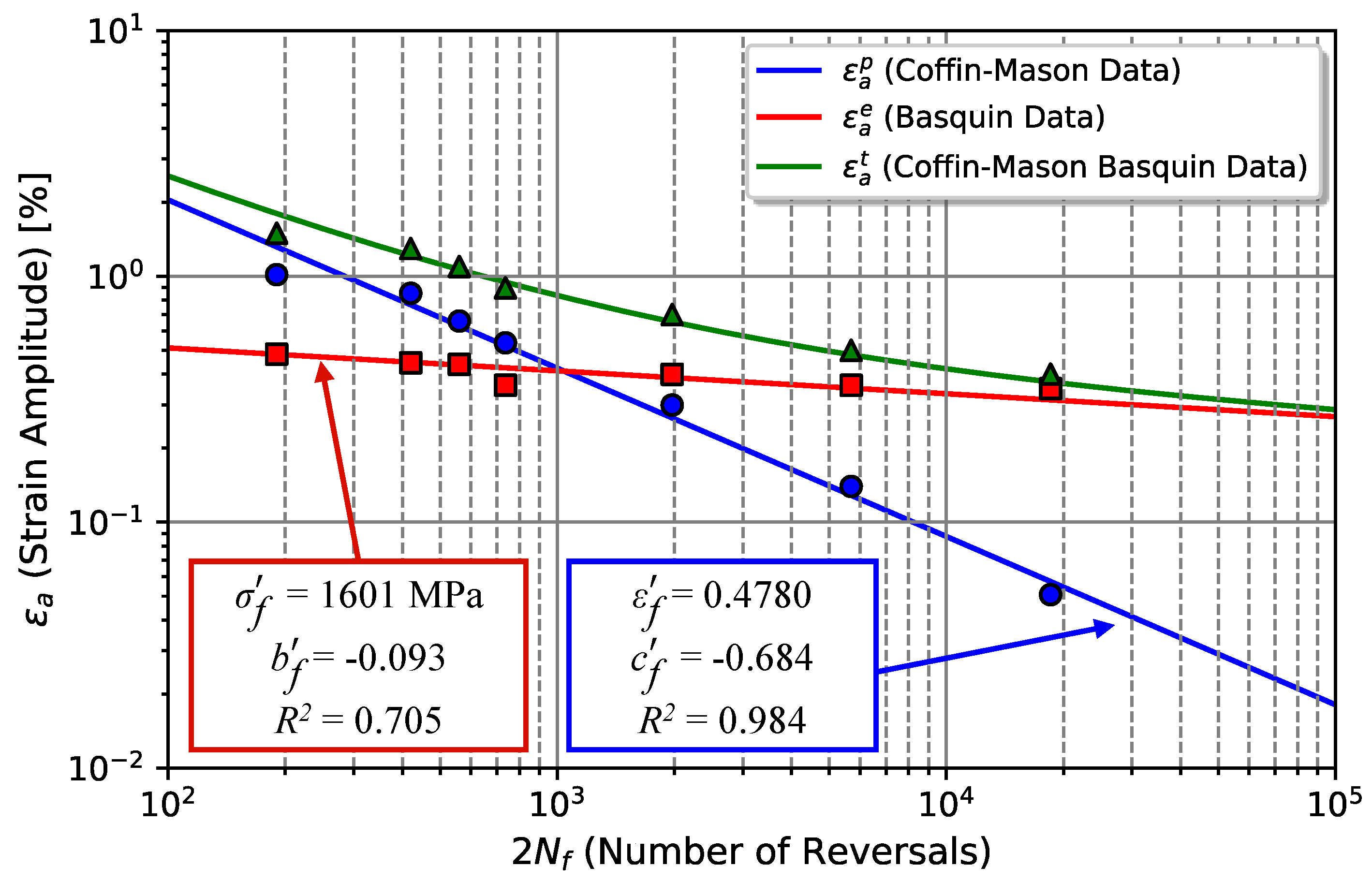
2.1. Strain-Based Life Method

This investigation intends to evaluate the fatigue strength of chromium-vanadium alloyed steel under cyclic straining conditions. Under stabilized conditions, steady-state hysteresis loops are taken into account for the use of fatigue strain-life methods, and the total strain range, Δ ε , is defined as
Δ ε = Δ ε e + Δ ε p = Δ σ E + Δ ε p ,
where Δ σ is the stress range and Δ ε is the strain range. The superscripts e and p denote the elastic and plastic parts of the strain.
In the presence of plastic deformations, the strain-based model suggested by Coffin–Mason and Basquin is more suitable [15,16,17], as has been proven in many research and engineering projects. For cyclic fatigue testing, the CMB relationship relates the number of cycles to failure, N f , with the total strain amplitude ε a t , indirectly using the number of reversals, 2 N f , such as
ε a t = Δ ε e 2 + Δ ε p 2 = σ f E 2 N f b f + ε f 2 N f c f .
where E is the longitudinal elasticity modulus, σ f is the fatigue strength coefficient, ε f is the fatigue ductility coefficient, b f is the fatigue strength exponent, and c f is the fatigue ductility exponent. The transition point at which both elastic and plastic strain components have the same weight for fatigue is given by Equation (3):
2 N f t = ε f E σ f 1 b f c f ,
Determination of the coefficients and exponents of the Equation (2) is performed for each stabilized loop of strain amplitude by first computing the elastic parameters and then the plastic ones.

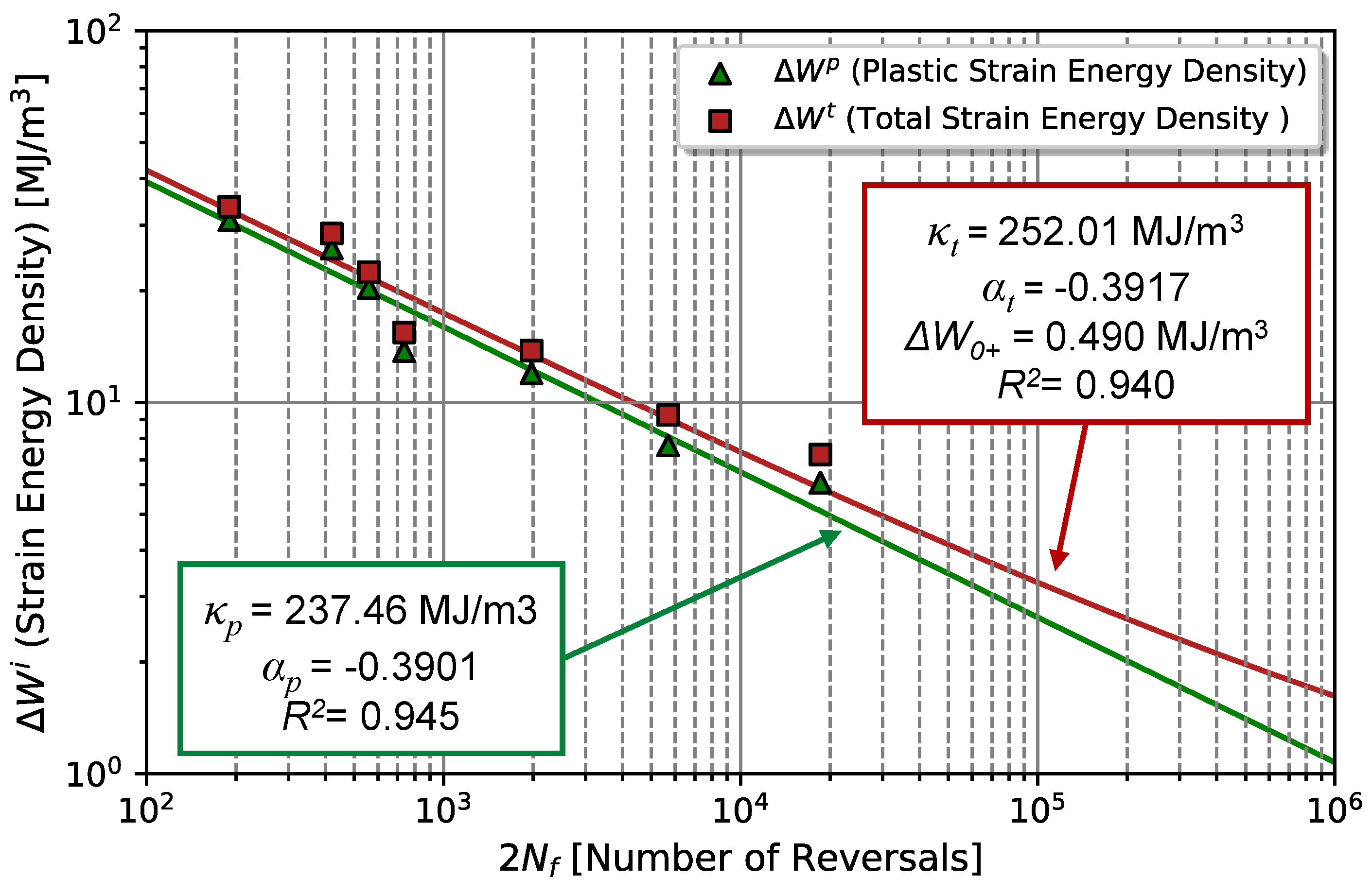
2.2. Total Energy Density-Life Method

In energy-based methods, the dissipated strain energy per cycle, Δ W p , is assumed to be the main contribution to the material fatigue damage process. Δ W p refers to the area within the hysteresis loop and may be related to the number of reversals to failure, 2 N f , such that [18]
Δ W p = κ p 2 N f α p ,
where κ p and α p are two unknowns determined from the experimental data using the least squares method. The model in Equation (4) may provide good predictions for fatigue in high-strength steels. Furthermore, this model becomes advantageous, since the parameter Δ W p remains almost constant throughout their lifetime, even for a large range of tempering temperatures, and increasing and decreasing slightly for lower and higher strain amplitude levels, respectively [18,19,20].
In spite of the applicability of the Δ W p parameter, this damage parameter is not suitable for longer fatigue lifetimes. To overcome this limitation, the total strain energy, Δ W t + , is usually considered as the damage parameter instead. Δ W t , written as
Δ W t + = Δ W p + Δ W e + ,
is suitable for both fully-reversed and non-null mean stress conditions. Thus, Δ W t + is defined as a sum of the hysteresis energy Δ W p and the elastic energy associated with the tensile stress per cycle, Δ W e + [21]. The model presented in Equation (5) can be further improved considering the residual fatigue resistance given by parameter Δ W 0 t . Δ W 0 t denotes the tensile elastic energy at the material fatigue limit, and then Δ W 0 t becomes the parameter Δ W t more sensitive to the mean stress [18,21,22]. Equation (5) is now rewritten as
Δ W t + = κ t 2 N f α t + Δ W 0 t .
The parameter Δ W t + is almost independent of the strain ratio at a constant strain amplitude [22,23]. These observations make this approach very desirable for fatigue life analysis in low-cycle fatigue, for both smooth and notched components, because we only need to determine the value of Δ W p for the stabilized cycle for a given value of Δ ε t [24,25,26,27].

3. Cyclic Elasto-Plasticity in Fatigue

3.1. Cyclic Elasto-Plasticity Theory

Cyclic elasto-plastic behavior is investigated because it is an important characteristic for fatigue analysis in components that might reach loading levels higher than the yield strength of the material. The Chaboche hardening model has been widely used in various studies to characterize cyclic hardening behavior, mainly in steels. Chaboche kinematic hardening was developed considering the von Mises plasticity criterion, as expressed in this work:
F ( σ α , σ y ) = ( σ α ) : ( σ α ) ( σ y + R ) = 0 ,
where σ and α are, respectively, the deviatoric part of the stress tensor, σ , and the back stress tensor; α . σ y is the initial size of the elasticity limit surface; and R is the change in the size of the elasticity limit surface. If R > 0 , the elasticity limit surface expands, otherwise, F contracts. The direction and variation of the elasticity limit surface are given by the associative flow rule, following the normality principle, and written as
ε ˙ p = λ ˙ F σ ,
where ε ˙ p , the time rate of plastic strain tensor and λ ˙ denotes the plastic multiplier. The updating of the stress and strain-state variables is given by the consistency condition, f / θ θ ˙ = 0 , with θ being σ , α , or R. The plastic multiplier in Equation (8) is computed from the consistency condition, which ensures the Kuhn–Tucker conditions.
Prager developed a linear hardening rule [28]. However, linear hardening is not often observed for small deformation regimes [29].
α ˙ = 2 3 C ε p ˙ ,
Posteriorly, Amstrong and Frederick introduced the concept of dynamic recovery, originating the kinematic model [30]. The AF model permits consideration of ratcheting effects due to the incorporation of the recovery term. Later, Chaboche improved the fitting of the transition between elastic and plastic domains in the AF model, introducing n α back stress tensors [29]. Thus, Equation (10) is written in terms of the i-th component of back stress tensor, α i :
α ˙ i = 2 3 C i ε p ˙ γ i α i p ˙ ,
such that
α = i = 1 N α i ,
where C i and γ i are fitting parameters [29], and the effective plastic strain rate tensor, p ˙ , is given by
p ˙ = 2 3 ε ˙ p : ε ˙ p .
In accordance with various investigations, the usage of three components permits obtaining good predictions of ratcheting behavior [29,31]. Notice that, if the non-linear part of the back stress disappears in Equation (10), the back stress is given by the linear hardening model, as written in Equation (9).

3.2. Determination Hardening Parameters

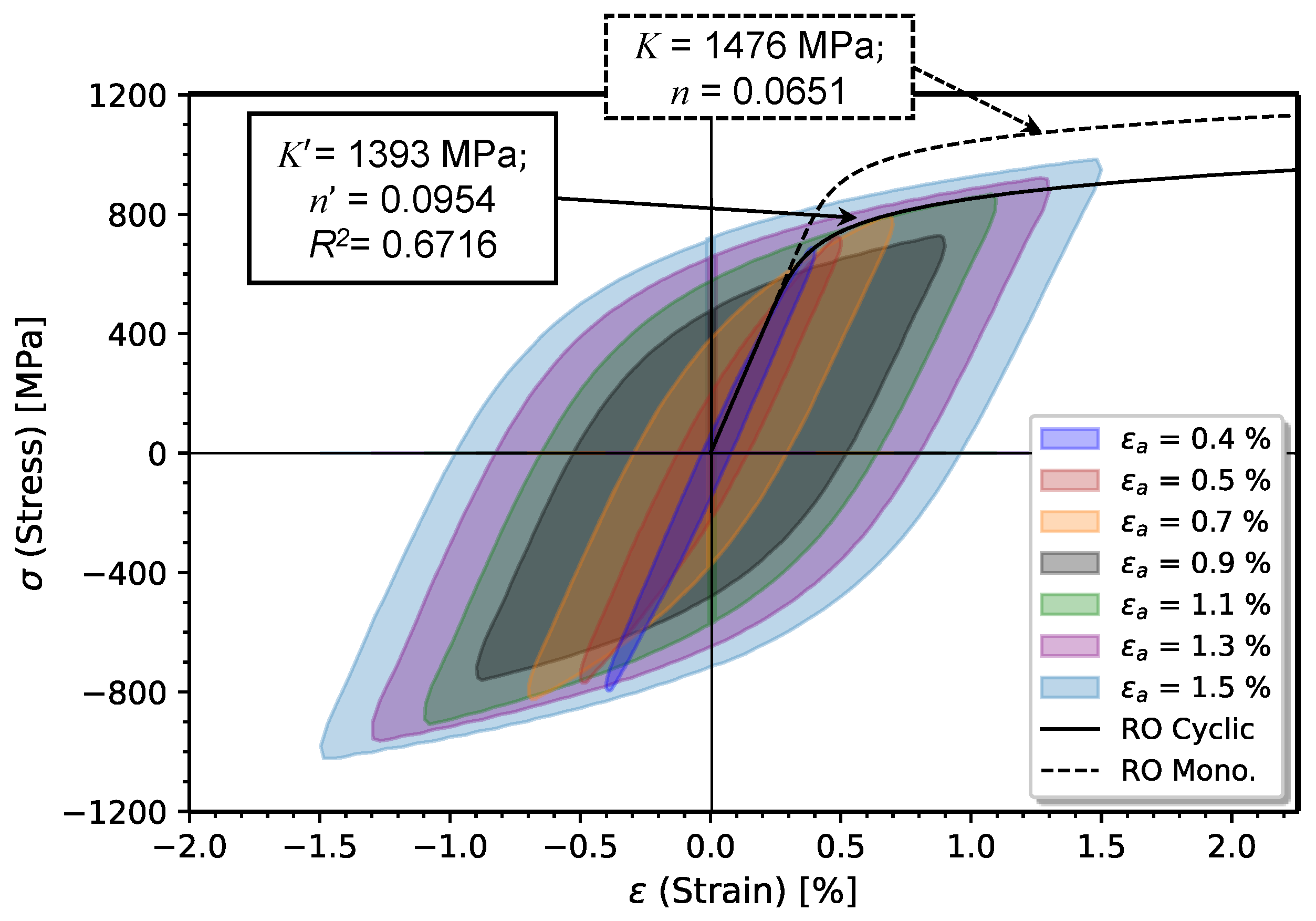
3.2.1. Cyclic Elasto-Plastic Ramberg–Osgood Model

The stable-cyclic elasto-plastic hardening of steels has been described using the Ramberg–Osgood model. This model relates the total strain, ε t , to the stress, σ , through a power law, in the form [32]:
ε a t = ε a e + ε a p = σ a E + σ a K 1 n ,
where E is the Young’s modulus, K is the cyclic hardening strength coefficient, and n is the cyclic strain hardening exponent. Ramberg–Osgood’s model (Equation (13)) is given by decomposing the total strain amplitude, ε a t , into its elastic, ε a e , and plastic, ε a p , parts.
In spite of being an old model, several researchers [33,34,35,36,37,38,39] recently used this equation model (13) to characterize the elasto-plastic behavior of a material under cyclic loadings, because this model is easy to apply and can also be correlated to fatigue life curves. In cyclic conditions, the cyclic strength hardening coefficient, K , and the cyclic strain hardening exponent, n , can be obtained with the linearization method and using the least-squares method. However, if the loading is monotonic, the monotonic strength coefficient, K, and the monotonic strength exponent, n, are computed as
n = log σ i / σ j log ε i p / ε j p ,
and
K = σ i ε i p n .
where σ j , ε j p > σ i , ε i p . Notice that the chosen ( σ , ε ) points must belong to the plastic regime.

3.2.2. Cyclic Elasto-Plastic Chaboche Hardening Model

The cyclic elasto-plastic model provided by Ramberg–Osgood (RO) is widely applicable to many different fatigue approaches. However, since this model is an empirical model, it has no hardening formulation; as a result, the RO model cannot predict transient effects such as cyclic hardening or softening, ratcheting, mean stress relaxation, etc. Instead, the Chaboche hardening model may be applied to deal with this concern. The Chaboche hardening model has been widely used in various studies to characterize cyclic hardening behavior, mainly in steels. Chaboche kinematic hardening was developed considering the von Mises plasticity criterion (Equation (7)).
For strain-controlled stable cyclic conditions, the kinematic hardening is written using Equation (16) as [29]:
σ a = σ y + Δ α 2 = σ y + R y + i = 1 n α C i γ i tanh γ i ε a p ,
where the parameters C i and γ i are determined by fitting the Equation (16), and R y denotes the variation of the elasticity limit surface for the stabilized-state hysteresis loop.
A useful feature of the Chaboche hardening model is the possibility to connect the isotropic hardening to the kinematic hardening behavior.The isotropic hardening permits a change in the size of the elasticity limit surface and is given by
R ˙ = b R R p ˙ ,
where R denotes the saturation of isotropic hardening and b denotes the rate of isotropic hardening. Both R and b are parameters depending on the material and temperature. Higher values of b indicate a faster saturation of the model, otherwise the yield surface tends to evolve more slowly. Integrating the Equation (17) results that
R = R 1 exp b p .
Equation (18) gives the size of the elasticity limit surface, and it may be used both in cyclic and monotonic loading conditions. Under strain-controlled cyclic conditions, the evolution of the elasticity limit surface (Equation (18)) may be represented in terms of the normalized maximum stress, as a function of the accumulated plastic strain, such that
R = R R = σ m a x ( N i ) σ m a x ( N i = 1 ) σ m a x ( N i = s ) σ m a x ( N i = 1 ) ,
with σ m a x ( N 1 ) , σ m a x ( N i = s ) , and σ m a x ( N i ) denoting the maximum stress corresponding to the first cycle, the stabilized cycle, and the i-th cycle, respectively. R denotes the difference between the value of yielding stress in the stabilized cycle and the value of yielding stress in the first cycle.
The value of R is dependent on the imposed deformation amplitude. Increasing the total strain amplitude, the quantity of hardening/softening, R , tends to increase with the maximum value, R , m a x . R , m a x indicates that, from a certain value of applied strain, which is around 2 or 3% for medium and high strength steels, the quantity of variation in the elasticity limit surface tends to remain unchanged [40,41,42]. The variation of R with the applied strain amplitude, ε a , is given by the decreasing power law, written as [43]
R = R , m a x 1 exp k 0 ε a ε 0 ,
where parameters k 0 and ε 0 are estimators for the amount of cyclic softening.
With respect to the hardening parameter that governs the saturation rate, b , this parameter may also be computed explicitly as
b = ln 1 R 2 N f Δ ε p .

4. Material and Procedures for Experimental and Numerical Approaches

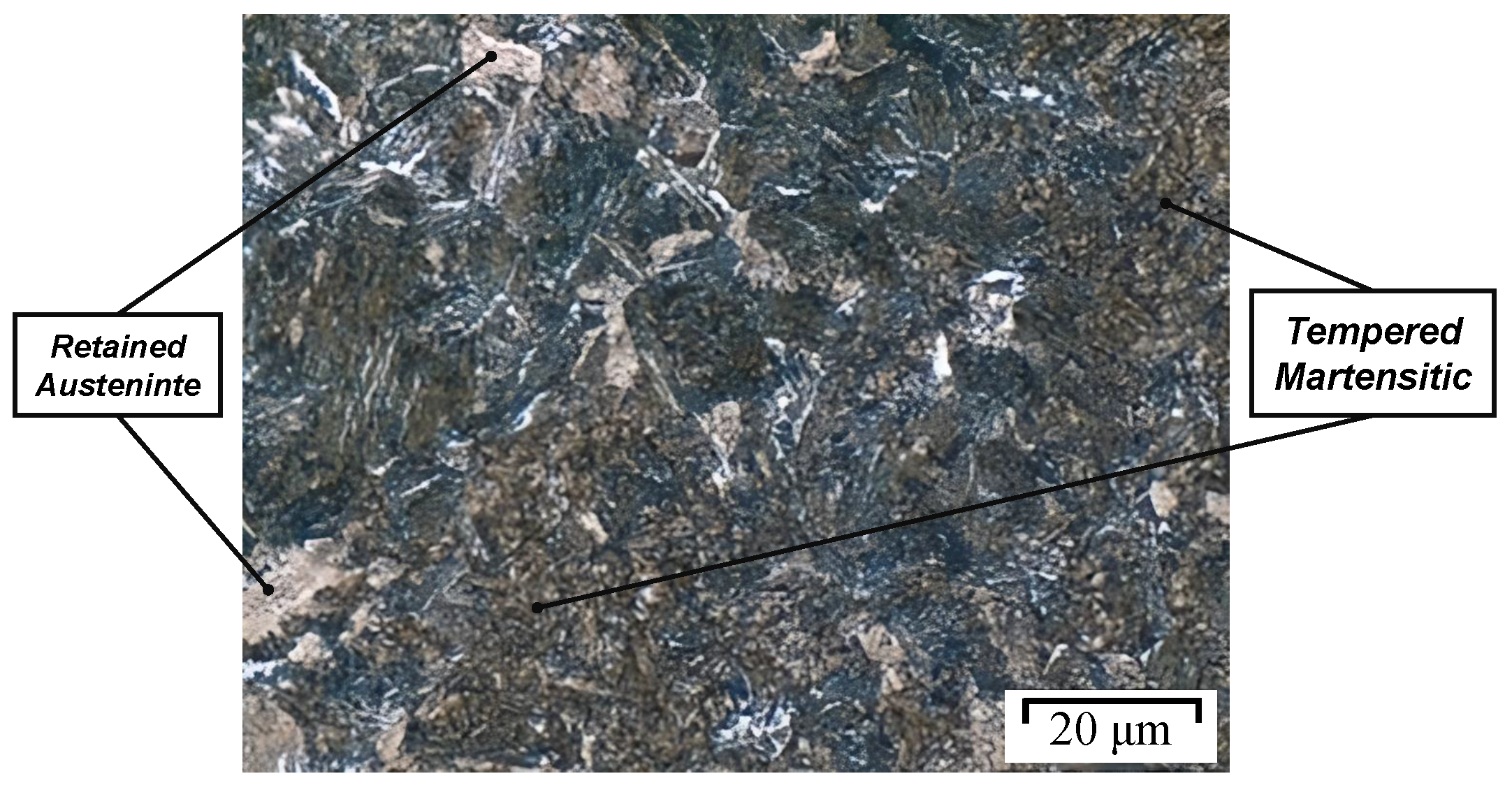
4.1. Chemical Composition and Microstructure

The steel under consideration is a hot-rolled chromium-vanadium alloyed steel 51CrV4. The samples were annealed, quenched at 850 ° C in an oil bath, and then tempered at 540–650 ° C for 2 h. Optical micrographs were created using an Olympus BX51 stereo microscope with a 1000-fold magnification on samples that had been etched with the agent HNO 3 . The etching process revealed a typical tempered martensite microstructure, with retained austenite with grain sizes of 20–30 μ m, as illustrated in the microstructure of Figure 2.
51CrV4 steel is a medium carbon alloyed steel, with an average carbon content of roughly 0.50%, alloyed with chromium and vanadium. On the one hand, chromium works as a stabilizing element for the ferrite, allowing improved corrosion and oxidation resistance. On the other hand, the inclusion of vanadium increases the mechanical resistance and hardness. The mechanical resistance and hardness are also increased due to the presence of silicon and manganese. Table 1 presents the chemical composition of each element composing 51CrV4 martensitic steel.

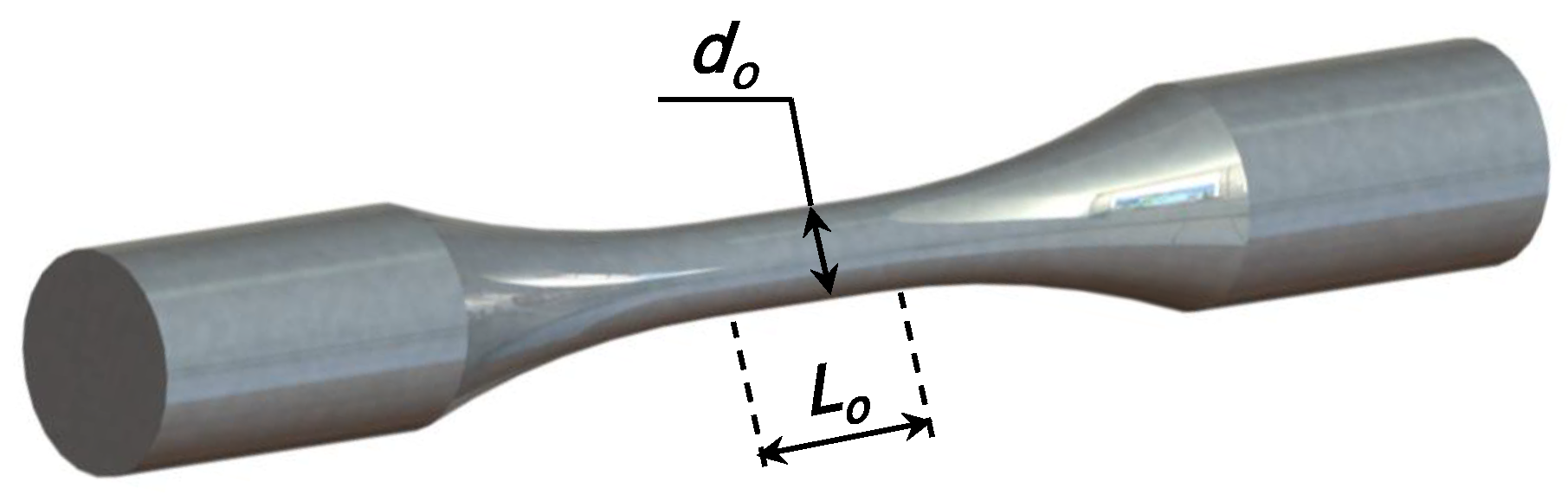
4.2. Monotonic and Cyclic Tests

Initially, the monotonic mechanical behavior of the quenched and tempered 51CrV4 steel with a Rockwell C of H R C = 38 HRC was investigated. Monotonic tensile tests were carried out using an Hydropulser Instron 8803 equipped with a high-resolution contact-free strain measurement (Fiedler laser extensometer P50) at room temperature under displacement-controlled conditions with a strain rate of 0.01 s 1 according to ASTM E8-03 [44]. Three samples were manufactured with an 8 mm diameter and 16 mm long cylindrical uniform-gauge length, as illustrated in Figure 3.
With respect to the fatigue testing samples, the same specimen geometry as illustrated in Figure 3, with a 8 mm diameter and 16 mm long cylindrical gauge, was considered. The considered fatigue testing method was the constant-step method under cyclic strain-controlled conditions, following the methodology described in the standard DIN 50100:2022-12 [45]. The strain was controlled using a dynamic clip gauge applied to the reference gauge length in the Hydropulser Instron 8803. Cyclic tests were conducted at the lab’s room temperature, for a strain ratio R ε = −1 and a strain rate of 0.01 s 1 . A triangular load-time function with a total strain amplitude of 0.4%, 0.5%, 0.7%, 0.9%, 1.1%, 1.3%, and 1.5% was considered. For each total strain amplitude condition, only a single specimen was considered. Table 2 summarizes the specimens’ geometry and setup inputs.

4.3. Empirical and Statistics Techniques

The statistical least-squares method was used to obtain the response curves of the fatigue strength and the elasto-plastic cyclic behavior of the material. Depending on the complexity of a statistical problem, a linear or non-linear method may be considered to estimate the regression parameters.
Considering the loss function, L ( 2 ) , is given by the ordinary least-squares (OLS) [46], in the case of a response function given by a linear function, as follows:
y = β 0 + β 1 x ,
with x and y denoting the design vector and respective response, respectively, the solution to the minimization problem results in the equation system in (23):
β ^ = arg min β ^ Ω | | y y ^ i | | 2 = X X 1 X y ,
where X is the design matrix, and X is its transposition.
On the other hand, if the response function is given by a non-linear function, optimization procedures are considered to find the value of the regression parameters. The fitting procedure follows an unconstrained numerical optimization scheme using the least-squares method. The objective function needs to be minimized according to the optimization problem:
β ^ = arg min β ^ Ω | | y y ^ i | | 2 = min β ^ Ω 1 N x i = 1 N x y i y ^ i y ^ i 2 ,
with N x denoting the size of vector x .
The minimization numerical problem is solved using the iterative method of Broyden–Fletcher–Goldfarb–Shanno (BFGS), with the recurrence equation given by [47]:
x k + 1 = x k + α k s s k ,
where in each iteration, k, the search direction, s k , is obtained using Hager–Zhang’s conjugate gradient method [48], for a maximum convergence error of 1.00 × 10 5 . The gradient of the objective function for x is computed using forward-mode automatic differentiation [49] and the step size, α k s , is always positive and assumed to be 1.0. With respect to the initial guess for a hessian matrix H 0 , this one is the identity matrix.

4.4. Finite Element Method

The finite element method implemented in the ANSYS FE code was considered to compare the cyclic material properties obtained from the statistical analysis of the experimental data. We considered a pure-displacement finite element formulation, for a cyclic small elasto-plastic deformation analysis of the material. The system of differential equations was solved for the displacement increment, Δ δ , according to the Newton–Raphson procedure considering the L2-Norm and using the direct sparse method with LDLT factorization for the matrix Equation (26):
K t Δ u = F e x t F i n t ,
with K t denoting the symmetric and positive-definite global tangent matrix, F e x t denoting the external forces applied at nodes, and F i n t representing the restoring loading vector. A single quadratic 20-node iso-parametric finite element with dimensions 1 × 1 × 1 following a full integration scheme of Gauss was considered. The von Mises plasticity criterion along with the combined Chaboche hardening model [29] was considered in the integration of the plasticity law using the return mapping algorithm, according to the Euler backward implicit scheme [50,51,52].

5. Results and Discussion

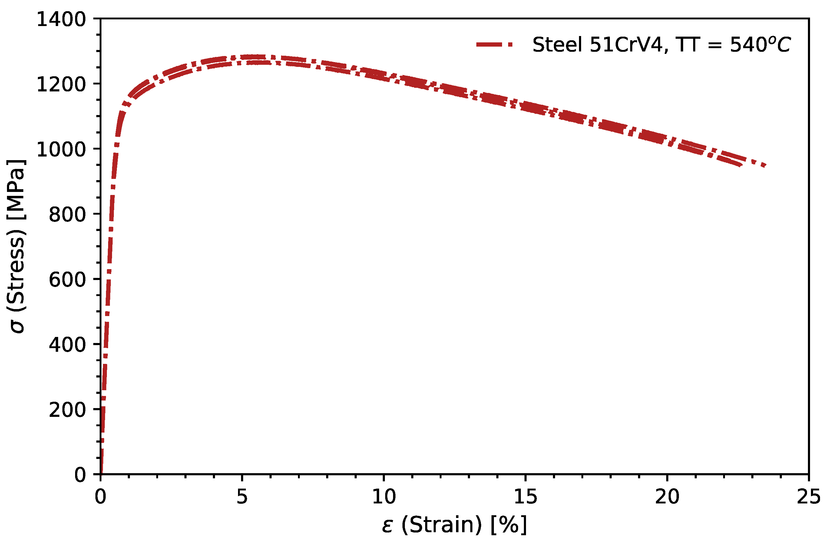
5.1. Mechanical Properties
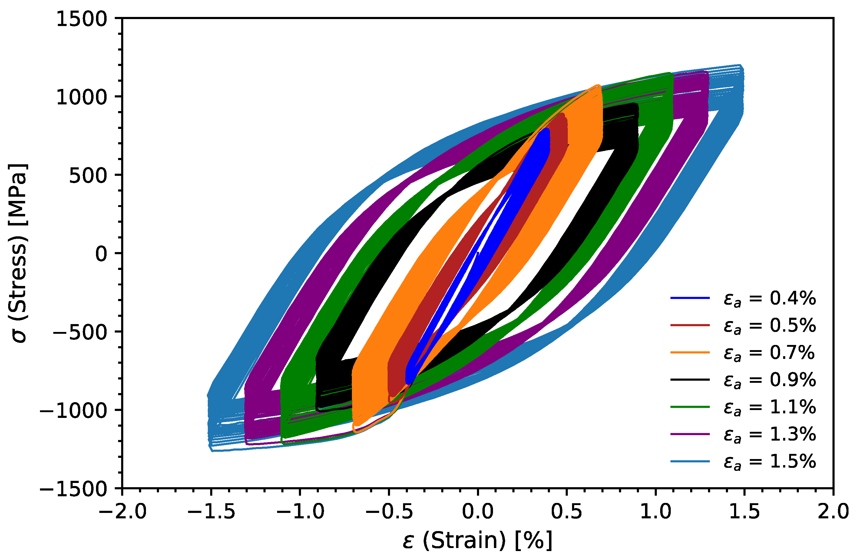
Monotonic tensile tests were carried out, until the failure of three specimens, as presented in Figure 4. Accordingly, the evolution of the monotonic behavior verified the high strength of the steel grade in the analysis, with a yield strength, σ 02 , and an ultimate tensile strength, σ u t s , around 1000 MPa and 1280 MPa, respectively.
With regards to the ductility, the ultimate strength corresponded to an ductility ε u t s = 5.90%. Despite the high resilience exhibited, this steel could also reach a high level of ductility at fracture, ε f , of 22.71%, which corresponds to an reduction in area R A f = 77.29%. Table 3 summarizes the mechanical properties obtained from the monotonic tensile tests under the testing conditions previously specified.
Figure 4 depicts the monotonic behavior of martensitic and tempered steel 51CrV4. The monotonic tensile tests revealed high-strength steel with a yield strength and an ultimate tensile strength around 1000 MPa and 1280 MPa, respectively. Additionally, a high ductility was exhibited, with values at fracture of 22.7%. A Young’s modulus, E, of 203.8 GPa was determined.

5.2. Cyclic Curve

The fatigue strength parameters in the low-cycle regime and the properties of cyclic hardening of the 51CrV4 were the aims of the present study. A criterion of 50% of the total fatigue life was considered for the determination of the fatigue curve under straining. Datasets obtained from the experiments were used to build a stabilized cyclic curve of Ramberg–Osgood.
Figure 5 depicts the fatigue tests performed for different strain ranges. The material presented a cyclic softening behavior for all applied strain amplitude levels. Regarding the sample tested for a strain amplitude of 0.9%, an inferior monotonic yield strength to the other samples was observed. Compared with the other datasets, it was possible to verify that the mechanical characteristics of this specimen were biased in relation to the observed average behavior. Consideration of this dataset allowed providing a more statistical behavior of the cyclic mechanical properties of the material.
Stabilised hysteresis loops were determined for each strain amplitude. In order to use a consensual criterion for consideration of the stress amplitude value, the criterion of half-life was assumed, because this criterion has been used in several investigations. Figure 6 depicts the hysteresis loops for each applied strain amplitude. There was a certain coherence in the growth of the maximum stress in each hysteresis loop and the applied strain amplitude, except for the test with a strain amplitude of 0.9%. The deviation in the behavior for this result goes back to what was verified in Figure 5.
The stabilized cyclic curve using Ramberg–Osgood’s model (Equation (13)) was considered. The elasto-plastic parameters for the cyclic behavior were obtained using linear regression, according to the least-squares method. The plastic strain amplitude was assessed as the width of the hysteresis loop measured over the axis σ = 0 . The elastic strain amplitude was evaluated from the decomposition of the total strain into elastic and plastic strain components, as described in Equation (1). Table 4 presents a summary of the elasto-plastic parameters for monotonic and cyclic loading conditions.
The regression model for determining the constants of K and n presented a coefficient of determination, R 2 , inferior to 0.67. Additionally, the tested strain levels encompassed the initial zone with a greater hardening material. For superior strain levels around 0.5%, the hardening presented from the monotonic curve was not so pronounced, and the error associated with the extrapolation of the cyclic curve was also inferior. The results of the cyclic and monotonic parameters with the increase in the hardening exponent were 0.0513 to 0.0954, revealing a reduction in the gradient of the cyclic hardening capacity of the material (around 14.04%). On the other hand, the hardening coefficient remained practically constant, K = 1393 MPa. With respect to the yield strength, σ 02 had the same meaning as σ 02 , however applied in cyclic conditions. Thus, considering a value 0.2% of residual plastic strain, σ 02 results in 769.96 MPa. In spite of the reference 0.2% being applicable for engineering practice, the cyclic yield strength computed for a 0.01% residual plastic strain provided a better adjustment in the mechanical behavior response [53], and therefore σ 01 = 578.5 MPa was considered. Considering σ 01 = 578.5 MPa, resulted in an amount of softening, R y , of −463.5 MPa.

5.3. Strain-Life Behavior

Table 5 presents a summary of the parameters obtained for Coffin–Manson and Basquin using the linear regression model. Coffin–Mason exhibited a better regression with a coefficient of determination, R 2 , equal to 0.984 against 0.705 with respect to Basquin’s model. Regarding the coefficients, the fatigue strength coefficient, σ f , was 1601.15 MPa, superior to σ u t s , and the fatigue ductility coefficient ε f was 47.80%, which is around double the monotonic strain at fracture, ε f . With respect to the exponent regressors, the fatigue strength exponent, b f , was equal to −0.093, whereas the fatigue ductility exponent, c f , was −0.684.
According to the Universal Slopes method, USM, [54], the coefficients σ f and ε f could be correlated to the monotonic tensile properties, such that σ f = 0.623 σ u t s 0.832 E 0.168 = 1865.87 MPa and ε f = 0.0196 ε 0.155 σ u t s / E 0.53 = 0.2291 , with the exponents b f and c f being constants of −0.09 and −0.69, respectively. Comparing strain-life parameters estimated using the USM method, one can verify that the USM was non-conservative (16.53%) with respect to σ f ; however, it was conservative in the estimation of ε f (52.07%). With regards of the exponents, a good agreement was observed, with relative errors of only around 3.23 and 8.82% for b f and c f , respectively.
Recently, Meggiolaro, and Castro [55] compared different estimation methods for the prediction of strain-life parameters. Accordingly, the outcomes, strain-life parameters, estimated regression based on the average values, and monotonic properties were very poor. In order to improve the estimation of strain-life parameters, Meggiolaro and Castro suggested an estimation model based on the median of individual parameters given the probability of distribution. The median model, MM, is suitable for a large range of materials, since it was developed based on 724 different steel grades, 81 aluminum alloys, and 15 titanium alloys. In a comparison with other estimation models, the MM model was shown to be more reliable for higher values of applied strain amplitude; however, for longer lifetimes, the MM model was less conservative than the USM model. Recently, the MM model was applied for Ti alloy components printed using electron beam melting, EBM, being shown to be conservative for longer lifetimes, but with a good fit with higher strain amplitude ranges [56].In the case of steels, the MM model suggests b f = 0.09 , ε f = 0.45 , and c f = 0.59 , and σ f = 1.5 σ u t s , which resulted in σ f = 1916.00 MPa. From a comparison with the experimental strain-life parameters, σ f remained non-conservative (19.66%); however, the estimation of ε f was improved, with an error around 5.86%. The relative error of c f was even higher (13.74%).
Figure 7 illustrates the Morrow, Basquin, and Coffin–Mason models in green, red, and blue lines, respectively. An estimation of the value for the transition from monotonic to low-cycle fatigue resistance was calculated for a limit value of strain amplitude corresponding to 2 reversals, ε a , t ( 2 N f = 2 ) , 30.49%. Moving to the transition point, the value corresponding to 2 N f , t was 1043 reversals, whose strain amplitude, ε a , t ( 2 N f , t ) , was 0.8243%. After this point, the plastic deformation effect decreased rapidly, and the fatigue life began to be governed by the component of elastic strain. When a transition region was defined from low-cycle to high-cycle, when the plastic strain reaches values inferior to 0.01%, according to the CMB model, the transition-life from low-cycle to the high-cycle regime, 2 N f , l c h c , was estimated to be 2.40 × 10 5 reversals.

5.4. Strain Energy Density Curves

The fatigue analysis method based on the strain energy density is another way to predict fatigue life. Using the total strain energy density parameters it is possible to assess fatigue resistance in longer lives. Figure 8 presents the fatigue-life curve considering the total strain energy density, and the plastic strain energy density as a function of the number of reversals.
From a qualitative point of view, the slopes of both models were very similar, which indicates a strong influence of the dissipative energy from plastic deformation. As the fatigue life was increased, the gradient of the models tended to diverge due to the influence of the parameter Δ W 0 + . Δ W 0 + induces a residual resistance associated with the fatigue limit of the material, and it was determined using the elastic strain energy computed for tensile stress. In the case of steel 51CrV4, the fatigue limit was estimated by considering 0.5% of the ultimate tensile strength, corrected using a load-type factor of 0.85.
From a quantitative analysis of the regression parameters, the similarity of the exponents α p = 0.391 and α t = 0.392 was expected. The differences in the coefficients κ p and κ t were of little significance, around 6.07%; that is, only 6.07% of the strain energy density was from the elastic strain energy density. For both models, a good fit was exhibited using the coefficient of determination, R 2 = 0.945 and R 2 = 0.940 . For a fatigue limit, σ a , l i m = 446.95 MPa, a elastic strain energy density, Δ W o + , of 0.49 was obtained MJ / m 3 . For a value 10% superior than Δ W o + , an infinite fatigue life, 2 N f , 90 % , of 1.09 × 10 7 reversals was found. For this fatigue life, the dissipated plastic energy, Δ W p , was 0.421 MJ / m 3 , which corresponds to a value of about 99.83% less than κ p . Table 6 summarizes the regression parameters obtained using least-squares methods for both the plastic strain energy density and total strain energy density models.
It is interesting to mention the effect of the chemical composition on the strain-life fatigue behavior. For example, with the presence of a spring steel with a higher carbon content, the yield strength, σ 02 , was typically higher, and hence a longer life was associated with the elastic strain component, and vice versa [19]. Quantitatively, this phenomenon was visible in the transition lifetime value, 2 N f , t , which was normally higher for lower values of σ 02 . Additionally, as σ 02 decreased, the plastic strain density, Δ W p , tended to increase.

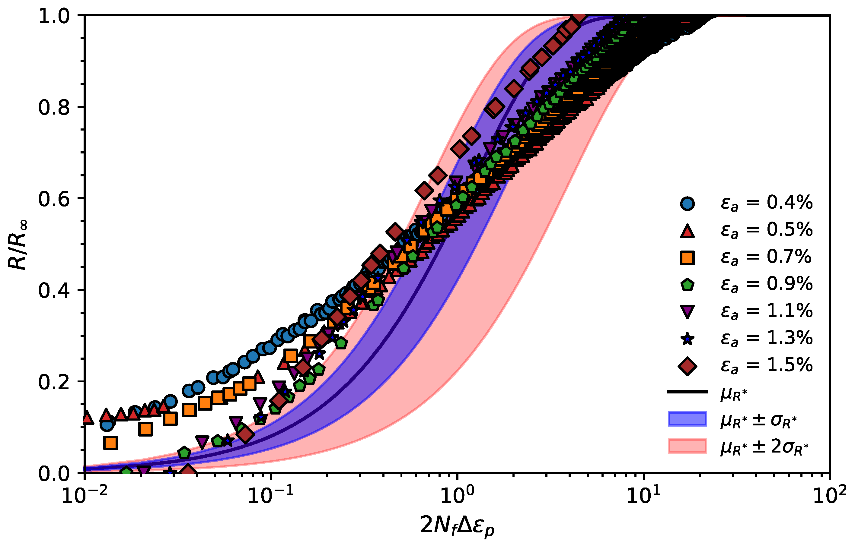
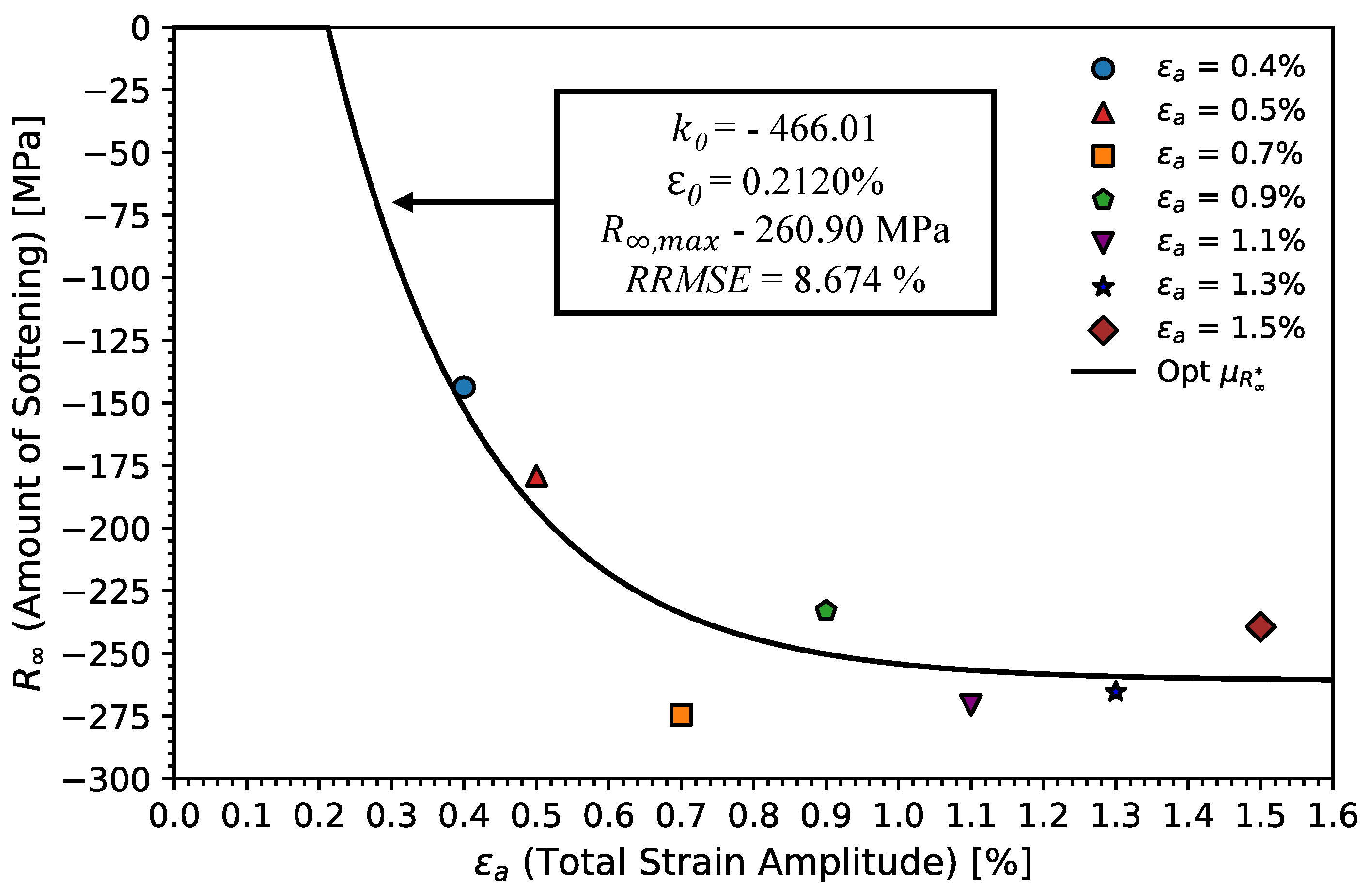
5.5. Hardening Parameters

Isotropic and kinematic hardening parameters were determined. The unconstrained optimization model presented in Equation (24) was used to determine the regression parameters of the hardening models.
Regarding the isotropic saturation rate parameter, b ^ , it is advisable to determine it according to the recommendations in [29,57]. Assuming a response parameter estimated as y ^ i = 1 + exp ( b ^ , i p i ) and y i = R i / R , Figure 9 shows the normalized maximum stress variation throughout the cyclic test up to the half-life in the scheme presented in [29]. The average curve and the respective 1- and 2-times standard deviations are presented. The experimental results showed a good behavior throughout the entire test in all applied strain ranges.
Comparing the average curve with the data obtained experimentally, we can see that there is a large variation between the average curve and the experimental data. This difference was greater in the initial test cycles. However, for higher strain gamma levels, the regression curve tends to describe the isotropic hardening behavior, as presented by the experimental data. Regarding the threshold saturation zone, it appears that there was not an exact saturation value for the experimental data, and therefore the isotropic model was unable to predict the real phenomenon.The value found by the optimization procedure was 0.8397, which is consistent with the values usually found for a wide range of materials, between 50 and 0.5 [57].
Regarding the variation of the amount of cyclic softening, Equation (20) was used to determine R , m a x . The amount of change in the size of the stabilized yield strength surface for a given deformation, R , was normalized using the yield strength, R . Thus, we defined the response, which was estimated as y ^ i = R ^ , m a x 1 exp k ^ 0 ε a , i ε ^ 0 and y i = R = | R , i | / σ y , i . The monotonic yield strength, σ y , considered was given by the arithmetic mean between σ p and σ 02 . The regressors R , m a x , k 0 and ε 0 were determined according to the unconstrained optimization scheme, with side bounds encompassing a pool permissible solution for the initial design vector of regressors, x = R , m a x , k 0 , ε 0 . The optimal solution was assumed to be that which had the lowest value of the objective function.
Figure 10 presents the regression obtained using the power model of Equation (20). According to Figure 10, the material began to exhibit a cyclic softening behavior for higher strain amplitudes than the threshold ε ^ 0 = 0.2120 % . Comparing the corresponding stress for ε ^ 0 with the cyclic proportional stress value σ p , and cyclic yield strength, σ y , resulted in differences of only 0.33 and 14.43%, respectively. The amount of softening tended to increase for strain amplitudes around 0.7 and 0.9%. This increase was given by a multiplicative factor, k 0 = 466.01 . For higher strain amplitude levels than 0.9%, the softening gradient decreased significantly, until it stabilized. The limiting value obtained using the optimization procedure was R ^ , m a x = 27.92 % , which corresponds to −260.90 MPa. This value, R ^ , m a x , corresponds to a strain amplitude level of 30.49%, which is the strain level for a lifetime of 2 reversals, as previously shown in Table 5. Table 7 presents the parameters determined for the isotropic hardening model.
Once the parameters of the isotropic hardening model had been determined, we determined the parameters of the kinematic hardening of the Chaboche model. The parameters C i and γ i were determined by fitting the Equation (16) to the cyclic Ramberg-Osgood Equation (13). The fitting model followed an unconstrained numerical optimization scheme using the least-squares method, such that the objective function needed to be minimized according to the optimization problem in Equation (24). The initial solution was generated using a pseudo-random number generator named Mersenne Twister, which is a 32-bit twisted GFSR random number generator MT19937 [58,59]. The side bounds for the parameters C i and γ i were set to limits of 10 7 and 10 7 . The Ramberg-Osgood fit curve, y , was defined up to the limiting condition defined by the strain amplitude for 1 cycle. Different Chaboche models with 1, 2, 3, and 4 back stresses were used and compared in terms of the objective function value. The non-linear models with 4 back stresses and the model with 3 non-linear and 1 linear back stresses were the ones that obtained the best results. Owing to Chaboche’s statement that 3 non-linear back stresses are sufficient to describe the initial hardening zone, and because only 1 linear back stress is used to describe the hardening for large strains, the model with 3 non-linear and 1 linear stresses was considered.Table 7 presents the values of the parameters obtained for this model. Using the values obtained in C i and γ i , we verified that the model was coherent with other works; that is, C 1 > C 2 > C 3 and γ 1 > γ 2 > γ 3 and C i > γ i .
Notice that in Figure 11-right, there was a good agreement between the evolution of decomposition components of the back stress with Chaboche’s model assumptions. The back stresses α 1 and α 2 made a greater contribution to the initial hardening of the model up to 2% plastic deformation. On the other hand, α 3 contributed gradually until a value of 18% plastic strain, saturating from there. Last, the linear component, α 4 , increased linearly from 0% to 30%, and then α 4 had a higher contribution in the large strain region. Figure 11-left compares the decomposition of the evolution of the cyclic yield stress, σ y , given by the sum of the back stress, α , with the size of the elasticity limit surface, R y , validating the fit of the Chaboche model to that of Ramberg-Osgood.

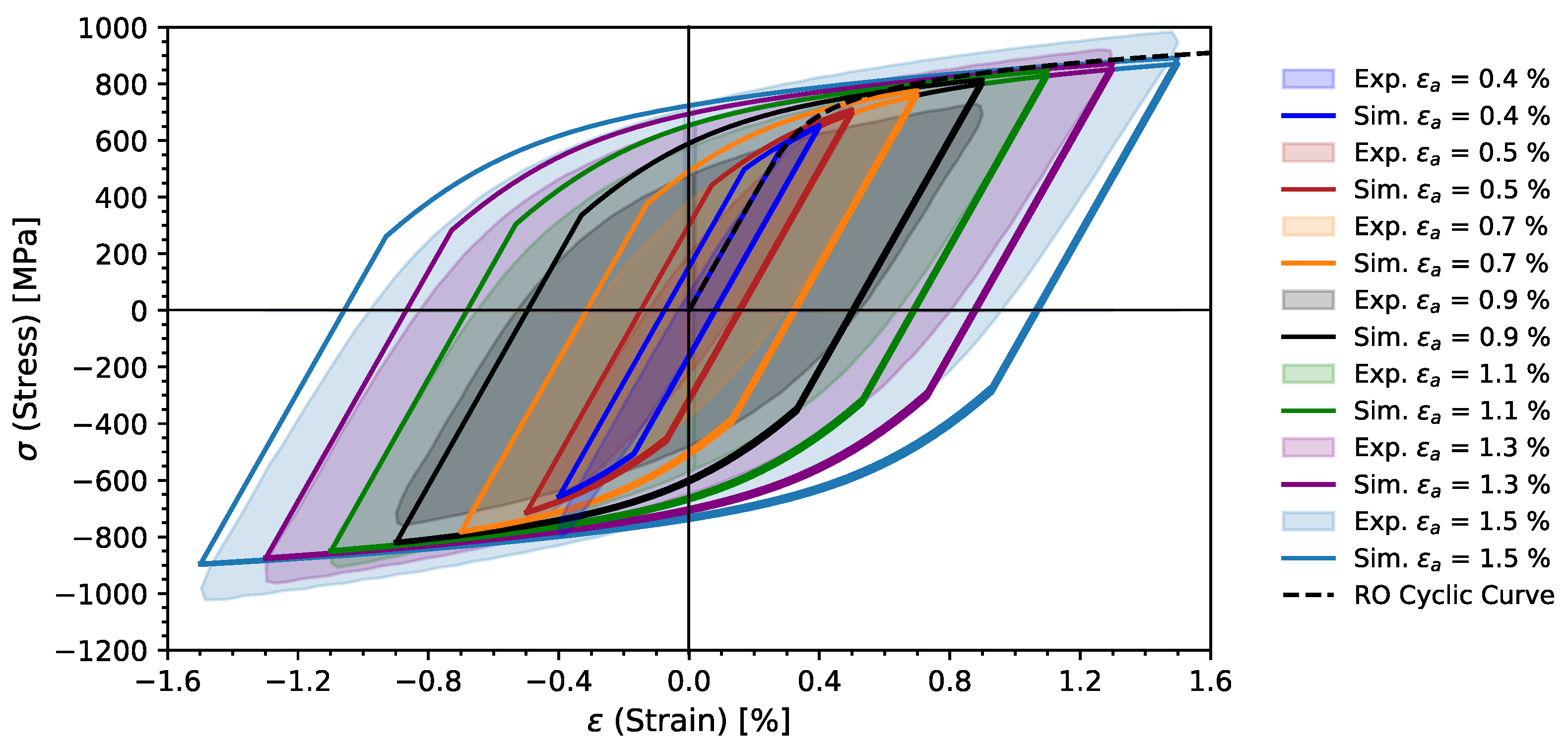
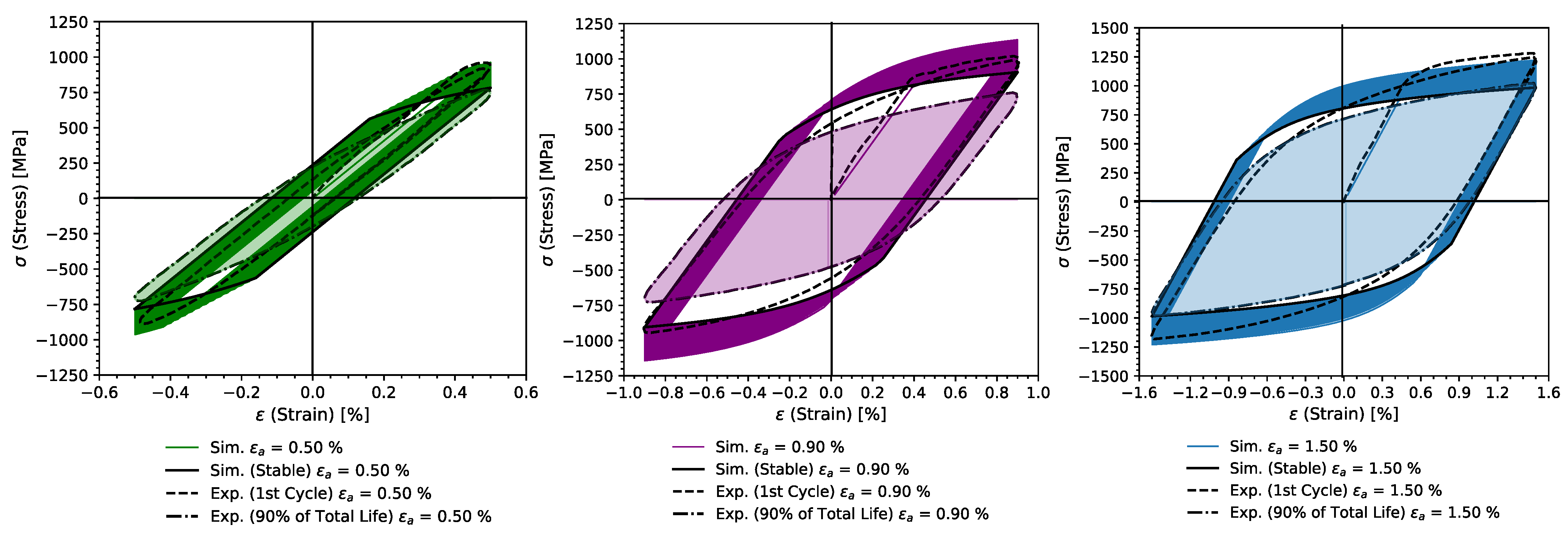
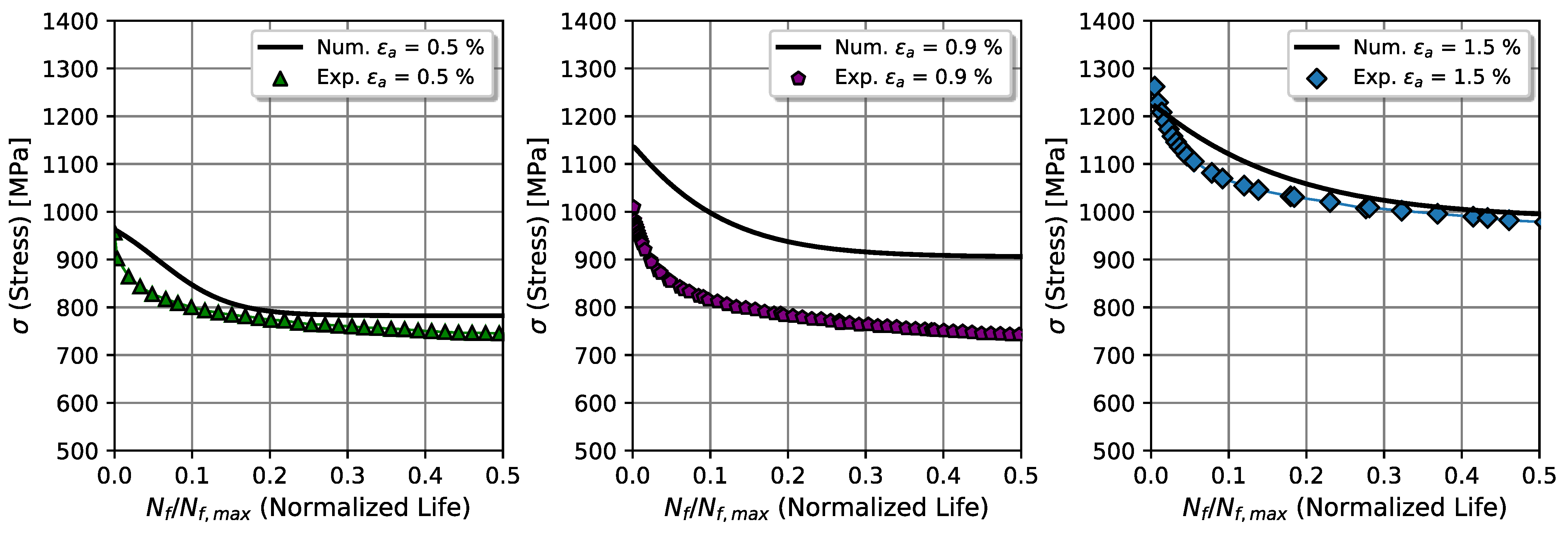
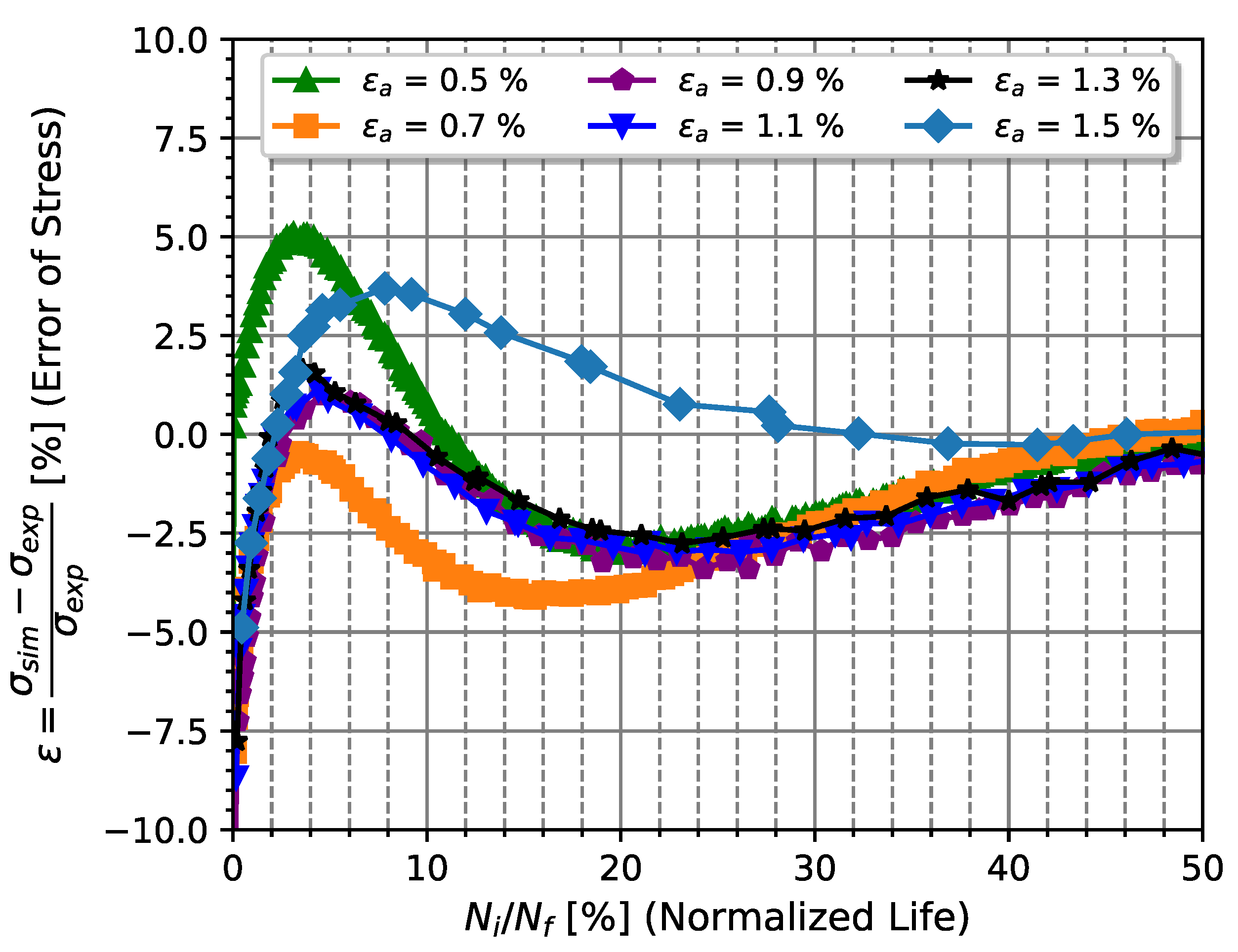
5.6. Cyclic Elasto-Plastic Response

The elasto-plastic cyclic response was compared with the experimental results obtained in the cyclic tests. A simulation for each strain amplitude level applied in the experiments was performed up to the number of failure cycles. The kinematic model was compared with the cyclic Ramberg-Osgood model and the experimental results. Then, the isotropic model was combined with the kinematic model, and the numerical results were compared with the experimental results.
Figure 12 compares the hysteresis loops for stabilized cyclic conditions obtained from the numerical and experimental models. Additionally, Figure 12 also presents a comparison of the Ramberg-Osgood curve with the maximum stress levels observed using the Chaboche kinematic hardening numerical model and considering the cyclic kinematic hardening properties in Table 7. In general, the maximum stress obtained from the Chaboche model showed a slight deviation in relation to the Ramberg-Osgood curve. This deviation tended to be higher as the strain amplitude was decreased. Additionally, from the comparison between the numerical and experimental outcomes, differences in the plastic strain energies were observed.
Regarding the transient behavior, this was analyzed considering all the numerical hysteresis cycles, and the experimental and stabilized cycles, as shown in Figure 13. The cyclic behavior shown in Figure 13 was obtained by considering the cyclic hardening model combined with the properties shown in Table 7. The three levels of the strain amplitude shown were 0.5% (small), 0.9% (medium), and 1.5% (large). Comparing the strain tests with 0.5 and 1.5%, it was observed that the numerical model was able to predict the maximum and minimum stress levels for both the first hysteresis loop and for the stabilized hysteresis loop. However, for an applied strain amplitude of 0.9%, a deviation was verified for both the first and for the stabilized hysteresis loop. This deviation is also observed in Figure 12, with the maximum stress of the hysteresis loop being lower than predicted by the Ramberg-Osgood curve. Since the isotropic hardening parameters were average values obtained for the test strain ranges, the deviation observed in Figure 13 for ε a = 0.9% was to be expected. With respect to the area developed by the plastic work, the Chaboche hardening model developed a greater dissipative energy, being more conservative in the fatigue analysis.
Another way of analyzing the evolution of isotropic hardening is the evaluation of the evolution of the maximum stress in each cycle, as represented in Figure 14. Figure 14 shows, in illustrative terms, a comparison o the numerical model results obtained using the combined Chaboche model. Experimentally, the softening gradient was greater up to approximately 5% of the total life. For normalized lifetimes greater than 10%, there was an almost linear softening, up to a normalized lifetime of 50%. Comparing the experimental data with the numerical results, it can be observed that, only as the strain amplitude increased did the lifetime associated with the stabilized behavior also tend to be higher. In the case of 0.5%, stabilization occurred to 20%, while for 0.9% stabilization occurred to approximately 50%. However, for a 1.5% applied strain amplitude, stabilization would occur for values greater than 50%.
As a way of evaluating the deviation of the numerical model with respect to the experiments, the variation of the relative error is shown in Figure 15. In order to evaluate the maximum relative error observed throughout the tests, the instant corresponding to 50% of the total failure lifetime was assumed as a reference value. This approach allowed us to understand that, for the applied strain ranges, the maximum relative errors occurred up to a lifetime of 10%, with error values that could vary between −10.0% and 5.0%. For lifetimes greater than 10%, the error was compressed into a range of −2.5 to 2.5%.

6. Conclusions

51CrV4 steel, with applicability in the railway components of the crossing nose and the frog of the turnout, was analyzed in terms of its fatigue resistance under strain-controlled conditions. The material showed a cyclic softening behavior, characteristic of high-strength steels. The criterion of 50% of the total life was considered, both for determination of the fatigue resistance properties and in determination of the Ramberg-Osgood cyclic elasto-plastic hardening curve parameters, resulting in n = 0.0954 and K = 1393 MPa (values very similar to the coefficient K for monotonic loading). With respect to the resistance curves, strain-life and energy-life approaches were considered. Application of the linear-squares method of the linearized power model was considered, resulting in a strain-life approach of σ f = 1601 MPa, ε f = 0.4780, b f = −0.093, and c f = −0.684. Applying the same method for the total strain energy density curves resulted in a κ t = 257 MJ/m 3 , α t = −0.3917, and a Δ W 0 + = 0.490 MJ/m 3 , which corresponds to a fatigue limit of 447 MPa.
Cyclic curve datasets were used to determine the kinematic and isotropic hardening parameters using unconstrained optimization procedures with a maximum convergence error of 1.00 × 10 5 . A kinematic hardening model with 3 non-linear plus 1 linear kinematic parameters was determined to be the best fitting model, with C 1 = 83,773.67 MPa, γ 1 = 582.52, C 2 = 16,778.05 MPa, γ 2 = 101.71, C 3 = 3013.29 MPa, γ 3 = 15.97, and C 4 = 854.52 MPa. Regarding the isotropic hardening parameters, these were obtained separately using unconstrained optimization and considering the least squares method. The value of the saturation rate was obtained using the normalized method of the maximum stress variation in each cycle, such that b = 0.8397. The saturation value of the yield surface size was estimated using a model that takes into account its variation as a function of the applied strain amplitude, resulting in R = 260.90 MPa.
The isotropic and kinematic hardening properties of the Chaboche model were used in the material numerical modeling, to validate them in relation to the experimental results. Initially, kinematic hardening properties were assigned in a purely kinematic model, for comparison with the Ramberg-Osggod stabilized loop results. The yield stress of the kinematic Chaboche model was assumed to be the cyclic stress determined using Ramberg-Osgood, σ f = 578.49 MPa. The results regarding the hysteresis loop were satisfactory. Afterward, numerical experiments were carried out considering the kinematic hardening model combined with the isotropic hardening model, for comparison with the experimental results. The deviation of the numerical model in relation to the behavior of the material obtained in the experiments was quantified, taking a value of 50% of the lifetime as a reference. It was found that the largest deviations occurred up to 20% of the total failure life of the material in a range of −10 to 5%, approximately.
As a result, the material properties determined in this investigation can be considered, not only in the analysis of crossing noses for railway infrastructure, but also in notched components, where local analyses based on elasto-plastic deformation and energy theories have more importance. In addition to contributing to the enrichment of the existing literature on the analysis of strain-life fatigue and cyclic plasticity hardening with the collected dataset, in the future, these datasets could be used for numerical analysis and also be correlated with other fatigue analyses, considering distinct tempering temperatures suitable for the spring steel 51CrV4.

Author Contributions

Conceptualization, V.M.G.G. and S.E.; methodology, V.M.G.G.; software, V.M.G.G.; validation, V.M.G.G., S.E., and A.M.P.D.J.; formal analysis, V.M.G.G.; investigation, V.M.G.G. and S.E.; resources, S.E. and A.M.P.D.J.; data curation, S.E.; writing—original draft preparation, V.M.G.G.; writing—review and editing, V.M.G.G., S.E., and A.M.P.D.J.; visualization, V.M.G.G.; supervision, S.E. and A.M.P.D.J.; project administration, S.E. and A.M.P.D.J.; funding acquisition, S.E. All authors have read and agreed to the published version of the manuscript.

Funding

This research was co-funded by the COMET program within the K2 Center “Integrated Computational Material, Process and Product Engineering (IC-MPPE)” (Project No 886385). This program was supported by the Austrian Federal Ministries for Climate Action, Environment, Energy, Mobility, Innovation and Technology (BMK) and for Labour and Economy (BMAW), represented by the Austrian Research Promotion Agency (FFG), and the federal states of Styria, Upper Austria and Tyrol. Additional funding was received from the European Union’s Horizon 2020 Programme Research and Innovation action under grant agreement No. 826255 (IN2TRACK2).

Institutional Review Board Statement

Not applicable.

Informed Consent Statement

Not applicable.

Data Availability Statement

The data presented in this study are available on request from the corresponding author. The data are not publicly available due to privacy restrictions.

Acknowledgments

The authors want to express their special thanks to Shift2Rail IN2TRACK projects and to the doctoral program iRail—Innovation in Railway Systems and Technologies funding by the Portuguese Foundation for Science and Technology, IP (FCT) through the PhD grant (PD/BD/143141/2019). Furthermore, a thank you to the Python, Julia, and Ansys communities.

Conflicts of Interest

The authors declare no conflict of interest.

References

  1. Wiest, M.; Daves, W.; Fischer, F.D.; Ossberger, H. Deformation and damage of a crossing nose due to wheel passages. Wear 2008, 265, 1431–1438. [Google Scholar] [CrossRef]
  2. Markine, V.L.; Steenbergen, M.J.M.M.; Shevtsov, I.Y. Combatting RCF on switch points by tuning elastic track properties. Wear 2010, 271, 158–167. [Google Scholar] [CrossRef]
  3. Xiao, J.; Zhang, F.; Qian, L. Numerical simulation of stress and deformation in a railway crossing. Eng. Fail. Anal. 2011, 18, 2296–2304. [Google Scholar] [CrossRef]
  4. Hamarat, M.; Papaelias, M.; Kaewunruen, S. Fatigue damage assessment of complex railway turnout crossings via Peridynamics-based digital twin. Sci. Rep. 2022, 12, 14377. [Google Scholar] [CrossRef] [PubMed]
  5. Eck, S.; Oßberger, H.; Oßberger, U.; Marsoner, S.; Ebner, R. Comparison of the fatigue and impact fracture behaviour of five different steel grades used in the frog of a turnout. Proc. Inst. Mech. Eng. Part F J. Rail Rapid Transit 2014, 228, 603–610. [Google Scholar] [CrossRef]
  6. Oßberger, U.; Kollment, W.; Eck, S. Insights towards condition monitoring of fixed railway crossings. Procedia Struct. Integr. 2017, 4, 106–114. [Google Scholar] [CrossRef]
  7. Yamada, Y.; Kuwabara, T. Materials for Springs; Springer: Berlin/Heidelberg, Germany, 2007. [Google Scholar] [CrossRef]
  8. Smith, W.F. Principles of Materials Science and Engineering, 3rd ed.; McGraw-Hill Book Company: Sydney, Australia, 1999. [Google Scholar]
  9. Li, H.Y.; Hu, J.D.; Li, J.; Chen, G.; Sun, X.J. Effect of tempering temperature on microstructure and mechanical properties of AISI 6150 steel. J. Cent. South Univ. 2013, 20, 866–870. [Google Scholar] [CrossRef]
  10. Wang, Z.; Liu, X.; Xie, F.; Lai, C.; Li, H.; Zhang, Q. Dynamic recrystallization behavior and critical strain of 51CrV4 high-strength spring steel during hot deformation. JOM 2018, 70, 2385–2391. [Google Scholar] [CrossRef]
  11. Zhang, L.; Gong, D.; Li, Y.; Wang, X.; Ren, X.; Wang, E. Effect of quenching conditions on the microstructure and mechanical properties of 51CrV4 spring steel. Metals 2018, 8, 1056. [Google Scholar] [CrossRef] [Green Version]
  12. Gomes, V.M.G.; De Jesus, A.M.; Figueiredo, M.; Correia, J.A.; Calcada, R. Fatigue Failure of 51CrV4 Steel Under Rotating Bending and Tensile. In Fatigue and Fracture of Materials and Structures: Contributions from ICMFM XX and KKMP2021; Springer International Publishing: Cham, Switzerland, 2022; Volume 8, pp. 307–313. [Google Scholar] [CrossRef]
  13. Brnic, J.; Brcic, M.; Krscanski, S.; Canadija, M.; Niu, J. Analysis of materials of similar mechanical behavior and similar industrial assignment. Procedia Manuf. 2019, 37, 207–213. [Google Scholar] [CrossRef]
  14. Han, X.; Zhang, Z.; Hou, J.; Thrush, S.J.; Barber, G.C.; Zou, Q.; Yang, H.; Qiu, F. Tribological behavior of heat treated AISI 6150 steel. J. Mater. Res. Technol. 2020, 9, 12293–12307. [Google Scholar] [CrossRef]
  15. Coffin, J.L.F., Jr. A study of the effects of cyclic thermal stresses on a ductile metal. Trans. Am. Soc. Mech. Eng. 1954, 76, 931–949. [Google Scholar] [CrossRef]
  16. Manson, S.S. Behavior of Materials under Conditions of Thermal Stress; National Advisory Committee for Aeronautics: Chantilly, VA, USA, 1954. [Google Scholar]
  17. Morrow, J.D. Cyclic plastic strain energy and fatigue of metals. Int. Frict. Damping Cyclic Plast. 1969, ASTM STP 378, 45–87. [Google Scholar] [CrossRef]
  18. Ellyin, F. Fatigue Damage, Crack Growth and Life Prediction, 1st ed.; Chapman and Hall: London, UK, 1997. [Google Scholar]
  19. Li, D.; Kim, K.; Lee, C. Low cycle fatigue data evaluation for a high-strength spring steel. Int. J. Fatigue 1997, 19, 607–612. [Google Scholar] [CrossRef]
  20. Branco, R.; Costa, J.D.; Antunes, F.V.; Perdigão, S. Monotonic and cyclic behavior of DIN 34CrNiMo6 tempered alloy steel. Metals 2016, 6, 98. [Google Scholar] [CrossRef] [Green Version]
  21. Golos, K.; Ellyin, F. Generalization of cumulative damage criterion to multilevel cyclic loading. Theor. Appl. Fract. Mech. 1987, 7, 169–176. [Google Scholar] [CrossRef]
  22. Branco, R.; Costa, J.D.; Borrego, L.P.; Wu, S.C.; Long, X.Y.; Zhang, F.C. Effect of strain ratio on cyclic deformation behaviour of 7050-T6 aluminum alloy. Int. J. Fatigue 2019, 129, 105234. [Google Scholar] [CrossRef]
  23. Mahtabi, M.J.; Shamsaei, N. A modified energy-based approach for fatigue life prediction of superelastic NiTi in presence of tensile mean strain and stress. Int. J. Mech. Sci. 2016, 117, 321–333. [Google Scholar] [CrossRef] [Green Version]
  24. Branco, R.; Costa, J.D.; Borrego, L.P.; Antunes, F.V. Fatigue life assessment of notched round bars under multi-axial loading based on the total strain energy density approach. Theor. Appl. Fract. Mech. 2018, 97, 340–348. [Google Scholar] [CrossRef]
  25. Callaghan, M.D.; Humphries, S.R.; Law, M.; Ho, M.; Bendeich, P.; Li, H.; Yeung, W.Y. Energy-based approach for the evaluation of low cycle fatigue behaviour of 2.25 Cr–1Mo steel at elevated temperature. Mater. Sci. Eng. A 2016, 527, 5619–5623. [Google Scholar] [CrossRef]
  26. Correia, J.A.F.O.; Apetre, N.; Arcari, A.; De Jesus, A.M.P.; Muñiz-Calvente, M.; Calçada, R.; Berto, F.; Fernández-Canteli, A. Generalized probabilistic model allowing for various fatigue damage variables. Int. J. Fatigue 2017, 100, 187–194. [Google Scholar] [CrossRef]
  27. Zhu, S.P.; Liu, Y.; Liu, Q.; Yu, Z.Y. Strain energy gradient-based LCF life prediction of turbine discs using critical distance concept. Int. J. Fatigue 2018, 113, 33–42. [Google Scholar] [CrossRef]
  28. Prager, W. Recent developments in the mathematical theory of plasticity. Int. J. Plast. 1949, 20, 235–241. [Google Scholar] [CrossRef]
  29. Chaboche, J.L. A review of some plasticity and viscoplasticity constitutive theories. Int. J. Plast. 2008, 24, 1642–1693. [Google Scholar] [CrossRef]
  30. Frederick, C.O.; Armstrong, P.J. A mathematical representation of the multiaxial Bauschinger effect. Mater. High Temp. 2007, 24, 1–26. [Google Scholar] [CrossRef]
  31. Rezaiee-Pajand, M.; Sinaie, S. On the calibration of the Chaboche hardening model and a modified hardening rule for uniaxial ratcheting prediction. Int. J. Solids Struct. 2009, 46, 3009–3017. [Google Scholar] [CrossRef] [Green Version]
  32. Ramberg, W.; Osgood, W.R. Description of Stress-Strain Curves by Three Parameters; National Advisory Committee for Aeronautics: Chantilly, VA, USA, 1943; Volume 902. [Google Scholar]
  33. Nejad, R.M.; Berto, F. Fatigue fracture and fatigue life assessment of railway wheel using non-linear model for fatigue crack growth. Int. J. Fatigue 2021, 153, 106516. [Google Scholar] [CrossRef]
  34. Correia, J.A.F.O.; da Silva, A.L.; Xin, H.; Lesiuk, G.; Zhu, S.P.; de Jesus, A.M.P.; Fernandes, A.A. Fatigue performance prediction of S235 base steel plates in the riveted connections. Structures 2021, 30, 745–755. [Google Scholar] [CrossRef]
  35. Qiang, B.; Liu, X.; Liu, Y.; Yao, C.; Li, Y. Experimental study and parameter determination of cyclic constitutive model for bridge steels. J. Constr. Steel Res. 2021, 183, 106738. [Google Scholar] [CrossRef]
  36. Kreithner, M.; Niederwanger, A.; Lang, R. Influence of the Ductility Exponent on the Fatigue of Structural Steels. Metals 2023, 13, 759. [Google Scholar] [CrossRef]
  37. Nejad, R.M.; Berto, F. Fatigue crack growth of a railway wheel steel and fatigue life prediction under spectrum loading conditions. Int. J. Fatigue 2022, 153, 106516. [Google Scholar] [CrossRef]
  38. Hu, Y.; Shi, J.; Cao, X.; Zhi, J. Low cycle fatigue life assessment based on the accumulated plastic strain energy density. Materials 2021, 14, 2372. [Google Scholar] [CrossRef]
  39. Souto, C.D.; Gomes, V.M.G.; Da Silva, L.F.; Figueiredo, M.V.; Correia, J.A.F.O.; Lesiuk, G.; Fernandes, A.A.; De Jesus, A.M.P. Global-local fatigue approaches for snug-tight and preloaded hot-dip galvanized steel bolted joints. Int. J. Fatigue 2021, 153, 106486. [Google Scholar] [CrossRef]
  40. Hu, F.; Shi, G. Constitutive model for full-range cyclic behavior of high strength steels without yield plateau. Constr. Build. Mater. 2018, 162, 596–607. [Google Scholar] [CrossRef]
  41. Wang, Y.B.; Li, G.Q.; Cui, W.; Chen, S.W.; Sun, F.F. Experimental investigation and modeling of cyclic behavior of high strength steel. J. Constr. Steel Res. 2015, 104, 37–48. [Google Scholar] [CrossRef]
  42. Jia, C.; Shao, Y.; Guo, L.; Liu, H. Cyclic behavior and constitutive model of high strength low alloy steel plate. Engineering Structures. J. Constr. Steel Res. 2020, 217, 110798. [Google Scholar] [CrossRef]
  43. Möller, B.; Tomasella, A.; Wagener, R.; Melz, T. Cyclic Material Behavior of High-Strength Steels Used in the Fatigue Assessment of Welded Crane Structures with a Special Focus on Transient Material Effects. SAE Int. J. Engines 2017, 10, 331–339. Available online: https://www.jstor.org/stable/26285046 (accessed on 31 March 2022). [CrossRef]
  44. ASTM E8-03; Load Controlled Fatigue Testing—Standard Test Methods for Tension Testing of Metallic Materials. American Society for Testing and Materials: West Conshohocken, PA, USA, 2017; pp. 1–23. [CrossRef]
  45. DIN 50100; Load Controlled Fatigue Testing—Execution and Evaluation of Cyclic Tests at Constant Load Amplitudes on Metallic Specimens and Components. Standard by Deutsches Institut Fur Normung E.V. (German National Standard): Berlin, Germany, 2022; Volume 217, pp. 1–114.
  46. Montgomery, D.C.; Runger, G.C. Applied Statistics and Probability for Engineers, 6th ed.; Wiley: Hoboken, NJ, USA, 2013. [Google Scholar]
  47. Montgomery, J.R.; Ning, A. Engineering Design Optimization, 1st ed.; Cambridge University Press: Cambridge, UK, 2021. [Google Scholar]
  48. Hager, W.W.; Zhang, H. Algorithm 851: CG DESCENT, a Conjugate Gradient Method with Guaranteed Descent. ACM Trans. Math. Softw. 2006, 32, 113–137. [Google Scholar] [CrossRef]
  49. Revels, J.; Lubin, M.; Papamarkou, T. Forward-mode automatic differentiation in Julia. arXiv 2016, 8, 3–30. [Google Scholar] [CrossRef]
  50. Bednarcyk, B.A.; Aboudi, J.; Arnold, S.M. The equivalence of the radial return and Mendelson methods for integrating the classical plasticity equations. Comput. Mech. 2008, 41, 733–737. [Google Scholar] [CrossRef] [Green Version]
  51. Krieg, R.D.; Krieg, D. Accuracies of numerical solution methods for the elastic-perfectly plastic model. J. Press. Vessel Technol. 1977, 99, 510–515. [Google Scholar] [CrossRef]
  52. Hughes, T.J. Numerical implementation of constitutive models: Rate-independent deviatoric plasticity. Theor. Found.-Large-Scale Comput. Nonlinear Mater. Behav. 1984, 6, 29–63. [Google Scholar] [CrossRef]
  53. Mohanty, S.; Soppet, W.K.; Barua, B.; Majumdar, S.; Natesan, K. Modeling the cycle-dependent material hardening behavior of 508 low alloy steel. Exp. Mech. 2017, 57, 847–855. [Google Scholar] [CrossRef]
  54. Muralidharan, U.; Manson, S.S. A modified universal slopes equation for estimation of fatigue characteristics of metals. J. Eng. Mater. Technol. 1988, 110, 55–58. [Google Scholar] [CrossRef]
  55. Meggiolaro, M.A.; Castro, J.T.P. Statistical evaluation of strain-life fatigue crack initiation predictions. Int. J. Fatigue 2004, 26, 463–476. [Google Scholar] [CrossRef]
  56. Petruz-Comas, A.D.; González-Estrada, O.A.; Martínez-Díaz, E.; Villegas-Bermúdez, D.F.; Díaz-Rodríguez, J.G. Strain-Based Fatigue Experimental Study on Ti–6Al–4V Alloy Manufactured by Electron Beam Melting. J. Manuf. Mater. Process. 2023, 7, 25. [Google Scholar] [CrossRef]
  57. Basan, R.; Franulović, M.; Prebil, I.; Kunc, R. Study on Ramberg-Osgood and Chaboche models for 42CrMo4 steel and some approximations. J. Constr. Steel Res. 2017, 136, 65–74. [Google Scholar] [CrossRef]
  58. Matsumoto, M.; Kurita, Y. Twisted gfsr generators. ACM Trans. Model. Comput. Simul. 1992, 2, 179–194. [Google Scholar] [CrossRef] [Green Version]
  59. Matsumoto, M.; Nishimura, T. Mersenne twister: A 623-dimensionally equidistributed uniform pseudorandom number generator. ACM Trans. Model. Comput. Simul. 1998, 8, 3–30. [Google Scholar] [CrossRef] [Green Version]
Figure 1. Illustration of a typical crossing nose geometry for a rail track.
Applsci 13 08308 g001
Figure 2. Optical micrographs of the chromium-vanadium alloyed steel at a tempering temperature of 540–650 ° C for 2 h. Identification of the tempered martensite and retained austenite (white phases).
Applsci 13 08308 g002
Figure 3. Geometry of the specimens used in the fatigue tests.
Applsci 13 08308 g003
Figure 4. Monotonic behavior under tensile loading of chromium-vanadium alloyed steel.
Applsci 13 08308 g004
Figure 5. 51CrV4 steel behavior under cyclic straining conditions until failure.
Applsci 13 08308 g005
Figure 6. Representation of the stable hysteresis loops obtained from the cyclic tests. Comparison of the elasto-plastic hardening model obtained from cyclic conditions with the monotonic elasto-plastic curve.
Applsci 13 08308 g006
Figure 7. Coffin–Manson and Basquin fatigue models for uniaxial strain-controlled conditions of 51CrV4 steel.
Applsci 13 08308 g007
Figure 8. Total and plastic strain energy densities at the half-life, as a function of the number of reversals to failure.
Applsci 13 08308 g008
Figure 9. Evolution of the normalized maximum stress during the cyclic test, until half of the total life was reached. Assessment of the isotropic model given by Chaboche using the estimators.
Applsci 13 08308 g009
Figure 10. Evolution of the amount of cyclic softening with the total strain amplitude applied.
Applsci 13 08308 g010
Figure 11. Evolution of the decomposition components of the back stress, total back stress, and the sum between the total back stress and size of the elasticity limit surface up to 30% plastic strain.
Applsci 13 08308 g011
Figure 12. Comparison of the numerical results given by Chaboche kinematic hardening model, experimental data, and cyclic Ramberg-Osgood model for steady-state cyclic conditions under various strain amplitudes.
Applsci 13 08308 g012
Figure 13. Comparison of the numerical results given by the combined hardening model and experimental data for the first hysteresis loop and the steady-state cyclic conditions.
Applsci 13 08308 g013
Figure 14. Comparison between the evolution of the maximum stress amplitude up to 50% of the total lifetime, obtained from the experiments and numerical outcomes.
Applsci 13 08308 g014
Figure 15. Comparison between the relative error in the evolution of the maximum stress amplitude up to 50% of the total life obtained from the experiments and numerical outcomes.
Applsci 13 08308 g015
Table 1. Standard chemical composition of the 51CrV4 steel grade, in % weight.
MaterialCSiMnCrVSPb
51CrV4 EN 1.8150.47–0.55≤0.400.70–1.100.90–1.20≤0.10–0.25≤0.025≤0.025
Table 2. Summary of the specimen geometry and fatigue testing setup.
d o [mm] L o [mm] A o [mm 2 ] R ε d ε /dt
816 50.24 −1.01.00%
Table 3. Mechanical properties obtained from monotonic tensile tests for steel 51CrV4.
E (GPa) σ 02 (MPa) σ uts (MPa) ε uts (%) ε f (%) R A f (%) H RC
203.8 1042 1277.33 5.90 22.71 77.29 38
± 1.2 ± 13.85 ± 5.03 ± 0.09 ± 0.68 ± 26.23 -
Table 4. Elasto-plastic parameters for monotonic and cyclic loading conditions.
E ( GPa ) σ y ( MPa ) K ( MPa ) n σ y ( MPa ) R y ( MPa ) K ( MPa ) n
203.50 1042.01365.180.0513578.5−463.51392.840.0954
Table 5. Parameters of Coffin–Manson and Basquin models (Equation (2)) obtained from the linear regression model.
Basquin M S E
0.172
σ f   [ MPa ]
1601.15
b f
0.093
ε a , t ( 2 N f = 2 )
[%]
2 N f , t
[reversals]
ε a , t ( 2 N f , t )
[%]
2 N f , l c h c
[reversals]
Coffin-Manson M S E
0.010
ε f   [ % ]
47.80
c f
0.684
30.4910430.82432.40 × 10 5
Table 6. Parameters of Equations (4) and (5) obtained from the linear regression model.
κ p ( MJ / m 3 ) α p κ t ( MJ / m 3 ) α t Δ W o + ( MJ / m 3 ) σ a , lim ( MPa ) 2 N f , 90 % Δ W p ( 2 N f , 90 % )
237.46 0.391 252.81 0.392 0.490 446.95 1.09 × 10 7 0.421
Table 7. Hardening parameters that defined the Chaboche isotropic and kinematic hardening model.
σ y ( MPa ) R ( MPa ) b σ y ( MPa ) n α C 1 ( MPa ) γ 1 C 2 ( MPa ) γ 2 C 3 ( MPa ) γ 3 C 4 ( MPa )
938.79−260.900.8397578.49483,773.67582.5216,778.05101.713013.2915.97854.52
Disclaimer/Publisher’s Note: The statements, opinions and data contained in all publications are solely those of the individual author(s) and contributor(s) and not of MDPI and/or the editor(s). MDPI and/or the editor(s) disclaim responsibility for any injury to people or property resulting from any ideas, methods, instructions or products referred to in the content.

