Article

Convolutional Neural Network for Segmenting Micro-X-ray Computed Tomography Images of Wood Cellular Structures

1
Materials Science and Engineering, University of Wisconsin–Madison, Madison, WI 53706, USA
2
Forest Biopolymers Science and Engineering, USDA Forest Service, Forest Products Laboratory, Madison, WI 53726, USA
3
Analytical Chemistry and Microscopy Laboratory, USDA Forest Service, Forest Products Laboratory, Madison, WI 53726, USA
4
Engineering Physics, University of Wisconsin–Madison, Madison, WI 53706, USA
5
Advanced Photon Source, Argonne National Laboratory, Lemont, IL 60439, USA
6
National Synchrotron Light Source II, Brookhaven National Laboratory, Upton, NY 11973, USA
*
Author to whom correspondence should be addressed.
Appl. Sci. 2023, 13(14), 8146; https://doi.org/10.3390/app13148146
Submission received: 16 June 2023 / Revised: 7 July 2023 / Accepted: 9 July 2023 / Published: 13 July 2023

Abstract

:
To further enhance the performance of wood products, improved tools are needed to study in situ cellular scale phenomena like mechanical deformations and moisture swelling. Micro-X-ray computed tomography (μXCT) using brilliant synchrotron light sources now has the spatial and temporal resolution for real-time visualization of phenomena in three-dimensional cellular structures. However, the tradeoff for speed includes the loss of intensity contrast between different types of materials within the imaged structure, such as cell wall and air in wood. This loss of contrast prevents traditional histogram-based segmentation methods from being used effectively. A new convolutional neural network (CNN) approach was therefore developed to segment fast μXCT images of wood into cell wall and air volumes. The fast μXCT and segmentation were demonstrated in the study of moisture swelling in loblolly pine (Pinus taeda) earlywood and latewood cellular structures conditioned at 0%, 33%, 75%, and 95% relative humidity (RH). The CNN segmentation results had a mean intersection over union (IoU) metric accuracy of 96%. Initial analysis of the swelling in the latewood revealed cell walls swelled about 25% when conditioned from 0% to 95% RH. Additionally, the widths of ray cell lumina in the transverse plane of latewood could be observed to increase at higher RH. The segmentation method presented here will facilitate future quantitative analyses in in situ μXCT studies of wood and other similar cellular materials.

1. Introduction

As a construction material, wood is often viewed favorably because of its mechanical performance, which in bending stiffness per weight is similar to or superior to man-made engineering composites [1], ease of machining, ready availability, and sustainability [2]. In addition to established wood construction materials, including solid dimensional lumber, plywood, oriented strand board, and laminated veneer lumber, new mass timber products like cross-laminated timber [3] and mass plywood panels [4] are being developed and becoming viable substitutes for concrete and steel in larger structures, such as mid-rise buildings and bridges. Because wood is a hierarchical cellular material (Figure 1) whose performance derives from the properties and organization of its smaller-scale components [5,6], continued progress towards realizing the full potential of wood and wood-based materials would be accelerated by improved understanding of behavior at these smaller length scales, especially observations of in situ dynamic processes. For example, wood cell walls absorb and desorb water depending on ambient conditions, which cause swelling and shrinking in wood that can lead to warping [7], splits [7], and wood-adhesive bondline failures [8]. However, the understanding of the swelling and shrinking in the cellular structure of wood, such as how much the cell wall material itself swells, how lumina volumes change in intact wood, and the dynamic swelling in real-time, is an active area of research in need of improved experimental approaches for adequate study [9].
Micro-X-ray computed tomography (μXCT) has been established as a valuable tool to make static observations in the cellular structure in intact wood specimens. Recent advancements at synchrotrons also show promise for utilizing μXCT in the study of in situ dynamic processes [11]. In μXCT, X-rays are used to illuminate a specimen volume and two-dimensional projection images of the specimen are acquired as the specimen is rotated. These images are then used to reconstruct the object’s three-dimensional internal structure by employing tomographic image reconstruction [12]. Select μXCT examples in wood research include moisture swelling and shrinking [13,14], adhesive penetration [15,16], identifying axial gas permeability pathways [17], deformations during tensile adhesive lap-shear specimens [18,19], deformations during three-point bending tests [20], and deformations caused by uniaxial compression [21].
Analyses of three-dimensional μXCT volumes often involve separating different classes of materials to visualize individual structures and quantify their volumes. A μXCT volume consists of a three-dimensional array of voxels in which each voxel has an intensity value. Segmentation is a method to separate the voxels into different object classes corresponding to different materials. When the intensity contrast between different object classes is sufficient, then the μXCT volume presents a multimodal intensity histogram. In such a volume, segmentation is readily achieved through traditional histogram thresholding techniques [22]. Histogram-based thresholding has been successfully utilized to visualize and quantify wood adhesive flow into wood [15,16,18,19], study swelling and shrinking of wood cell walls [13], and create models to simulate axial permeability [17].
However, previous μXCT studies in wood have primarily focused on capturing images of static specimens. High-speed, time-resolved μXCT is now realized at brilliant synchrotron light sources and can be used for real-time in situ μXCT observations [11]. These new capabilities will enable new innovative experiments to capture in situ dynamic processes at the cellular length scale in wood and forest products, such as in situ real-time observations of mechanical deformations, pressure and temperature changes, pyrolysis, chemical modifications like biorefinery pretreatments, and transport of water and other chemicals into and out of wood.
Before high-speed μXCT imaging can be effectively utilized to study wood, improved segmentation methods are needed because the imaging parameters used to gain high temporal resolution in high-speed μXCT, such as employing higher energy (>10 keV) polychromatic X-ray beams and propagation-based imaging, result in μXCT volume reconstructions with less differential contrast between materials. The lower contrast prevents traditional histogram thresholding techniques from being used. Propagation-based imaging is a type of phase contrast imaging in which Fresnel diffraction at interfaces between materials with different refractive indices, such as wood cell walls and air in wood, results in interference fringes recorded by the detector in the projection images [23]. Increases in sample to detector distance increase the differences between the peaks and valleys in the recorded interference fringes. Therefore, increasing the sample to detector distance to incorporate environmental chambers or mechanical testing fixtures further enhances interference fringes in the phase contrast images. In reconstructed transverse wood cross-sections, these phase contrast effects result in large grayscale intensity variations near the lumen-cell wall interfaces that further inhibit successful implementation of traditional histogram-based thresholding segmentation techniques [24].
Fortunately, machine learning segmentation approaches based on convolutional neural networks (CNN) show promise for segmenting X-ray computed tomography images with limited intensity variations between material classes [25]. U-Net is a CNN that was originally developed for fast and precise segmentation of biomedical images [26]. Given U-Net’s effectiveness for segmenting the cellular structure of HeLa cells in light microscopy images, U-net has promise for segmenting μXCT images of wood cellular structure. U-Net converts the image segmentation process into a pixel classification problem in which each specific pixel within an image is assigned to categories corresponding to different object classes [27]. To accomplish the pixel classification, the network is trained to learn from prepared reference images known as ground-truth images [28,29]. The two main steps in the training process algorithm are forward propagation and back propagation [26]. Initially, filter weights are randomly assigned. In forward propagation, the algorithm performs a first prediction of segmentation using these random weights. The prediction is compared with the ground-truth image and an error is calculated using an error minimization function. This error is then backpropagated through the network to adjust the weights for a better prediction in the next iteration. The process is continued until the error is completely minimized or reaches a predefined minimization value [27,28,29]. Essentially, this means that the network will learn filters that capture visual information [28]. The filters are tuned to capture features from the training images such as edges, orientations, and ultimately entire patterns. After being trained, U-Net takes as input a single-channel gray-scale image and outputs a multi-channel image where each channel contains the probability information of each pixel belonging to a particular class [26]. In the case here for wood cellular structure, there will be two classes consisting of cell wall material and air.
In this study, we employed a custom-built in situ μXCT relative humidity (RH) chamber designed to study cellular-scale swelling processes in wood and other hygroscopic materials. The RH chamber was used with fast propagation-based phase-contrast μXCT imaging to capture full tomogram data sets of wood in only 7.5 s. The goal was to develop μXCT protocols to meet the recognized need for new tools to study dynamic wood–water interactions at the cellular length scale [9]. However, the resulting μXCT volumes lacked sufficient contrast between the air and cell wall volumes. Therefore, traditional histogram-based thresholding segmentation methods failed. A new segmentation process based on U-Net CNN [26] was therefore developed and employed in this study to overcome the shortcomings of traditional segmentation methods. This new segmentation process will facilitate quantitative analyses of wood and similar cellular materials when fast μXCT imaging is used.

2. Materials and Methods

2.1. Sample Preparation

Earlywood and latewood micro-X-ray computed tomography (μXCT) specimens were extracted from loblolly pine (Pinus taeda L.). First, longitudinal-tangential sections with a nominal thickness of 50 µm, 150 µm, 500 µm, or 1 mm were cut using a Reichert (Vienna, Austria) sled microtome equipped with a disposable microtome blade. The sections measured 1 cm in the longitudinal direction. To aid in cutting, the wood was first saturated with water. An individual wood specimen was cut by hand along the longitudinal wood axis using a single edge razor blade under a Motic (Schertz, TX, USA) SMZ-168 stereomicroscope. A total of 24 specimens were prepared with three latewood and three earlywood specimens for each size.

2.2. Micro X-ray Computed Tomography (μXCT)

Fast phase-contrast μXCT experiments were carried out at the Advanced Photon Source beamline 2-BM-B at the Argonne National Laboratory (Argonne, IL, USA). Details of the beamline setup have been described elsewhere [30,31]. Imaging was performed using a filtered polychromatic X-ray illumination beam with a peak energy of about 25 keV. A 20-µm thick Ce-doped Lutetium Aluminum Garnet (LuAG:Ce) scintillator was positioned at a distance of 10 cm from the sample and used to convert the transmitted X-rays to visible light. The images were magnified by a 10× Mitutoyo (Kawasaki, Japan) long working-distance objective lens and recorded by a PCO.edge™ (Kelheim, Lower Bavaria, Germany) camera with a 2560 by 2160-pixel count. The experimental setup resulted in a 0.65 μm pixel size and produced a field-of-view of 1.664 mm by 1.404 mm. Each tomogram data set consisted of 1500 projections collected over a 180° rotation at 0.12° angular increments with 5 ms exposure time for each projection. Each 1500 projection tomogram data set took approximately 7.5 s to collect. White-field and dark-field images were also collected for each tomogram data set and used for intensity corrections. A white-field image was collected while the detector was irradiated without the sample’s obstruction, and the dark-field image was collected while the X-ray beam was blocked from the detector.
XCT imaging was performed on each wood specimen conditioned in absorption at RH values of 0% (dry air), 33%, 75%, and 95%. Before imaging, the specimen was placed into an external chamber for at least 24 h to condition at the given RH, which was controlled using desiccant or aqueous salt solutions (Table 1). The wood specimen was then transferred quickly from the external chamber to the in situ beamline RH chamber (Figure 2) and conditioned for 10 min at the corresponding RH step before imaging. The RH in the beamline chamber was controlled with an IntruQuest HumiSys™ HF (Coconut Creek, FL, USA) RH generator. The RH and temperature were measured inside the beamline chamber during imaging using a Sensirion (Staefa, Switzerland) SHT1x humidity sensor. The calibration of the temperature and RH sensor inside of the beamline chamber was verified using a Control Company (Webster, TX, USA) 4085 Traceable® Hygrometer Thermometer Dew Point Meter. The temperature ranged from 27 to 28 °C. After imaging, the sample was transferred to the external humidity chamber that was conditioned for the next higher RH step. Imaging for each RH step occurred on successive days to allow at least 24 h of conditioning. The process was repeated until all the wood specimens were imaged at each RH step.

2.3. Image Reconstruction

The tomogram data sets were reconstructed using Tomopy Python package [33]. The raw intensity data were normalized using the white-field and dark-field corrections to compensate for different detector pixel responses. The intensity data were then scaled between 0 and 1 by calculating the normalized data’s negative logarithm. Detector artifacts, such as ring artifacts and streaks, caused by the drift of the inhomogeneous X-ray beam or imperfections of the imaging detector system were not entirely removed by normalization. The detector artifacts were further reduced by employing stripe removal filtering in the sinograms using the combined wavelet–Fourier filtering technique [34]. The best results were obtained with the wavelet Daubechies 5 (db5) with a decomposition level of 10 and a smoothing factor of 3. Higher-order wavelet filters reduced the sharpness of the reconstructed images. The filter parameters were chosen as an optimization between artifact suppression and the preservation of the image object details. However, some streak artifacts persisted in the reconstructed images as are described later in the manuscript.
For reconstruction, both filtered back projection (FBP) and conjugate gradient least squares (CGLS) methods were initially performed and compared. FBP methods have previously been used in μXCT wood studies [18,19,20]. The FBP reconstruction method is based on the Fourier grid reconstruction algorithm and has the advantage of computational efficiency [35]. However, FBP reconstructions have the disadvantage of resulting in a noisier reconstruction when there is noise in the acquired projection data. The CGLS algorithm is an algebraic iterative reconstruction method based on numerical approximations determined by minimizing the difference between the forward projection of the reconstructed image with the acquired projection data using the conjugate gradient method [36]. Although the CGLS method is more computationally intensive than the FBP method, it has the advantage that the effect of noise in the projection images can be reduced by finding the optimum number of iterations [36]. In this work, the optimal iteration was 100. Lower numbers of iterations were tested to decrease the computation intensity. However, the lower numbers resulted in high-frequency noise in the reconstructed images. Figure 3 shows comparisons from the current experiments between FBP and CGLS reconstructed image slices and intensity line profiles. The CGLS reconstructed image is less noisy, which will be better for image segmentation and further analysis [36]. Therefore, the CGLS method was used for reconstructing the data for further analysis.

2.4. Post-Processing, Segmentation, and Visualization

Each reconstructed file consisted of 52.7 Gb of data with stacks of 2160 32-bit cross-sectional images stacked along the longitudinal direction of the wood samples. To reduce the amount of time during computations and make the segmentation process less memory intensive, the reconstructed gray-scale images were converted from 32-bit single-precision floating-point images to 8-bit unsigned integer images using ImageJ [37]. File sizes were further reduced for 50 µm, 150 µm, and 500 µm cross-section specimens by cropping images uniformly along a given stack length to remove excessive void spaces outside of the wood specimen.
A convolutional neural networks (CNN) image segmentation method was employed because traditional histogram-based thresholding segmentation methods still failed even with the improved CGLS reconstructions. The CNN was implemented in Wolfram (Champaign, IL, USA) Mathematica. The μXCT data processing, image reconstructions, and computations were performed using Python programming language [38]. ImageJ was used for visualization [37].

3. Results and Discussion

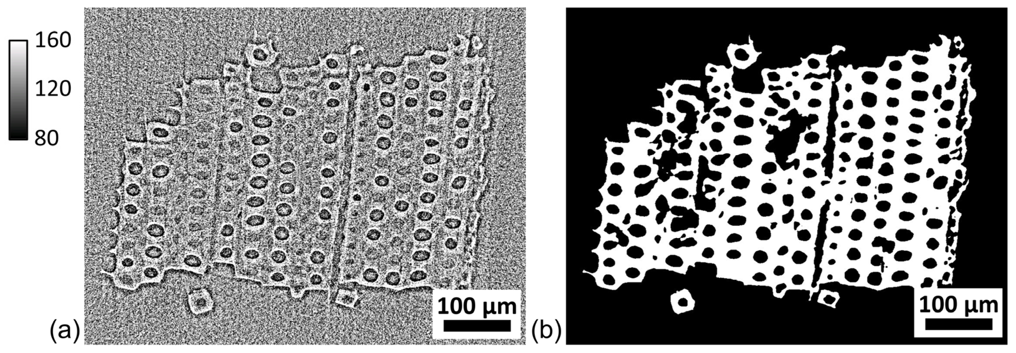
3.1. Reconstructed Grayscale Images

Representative latewood and earlywood reconstructions from 1 mm cross-section specimens are shown in Figure 4. The two material classes in the images are cell wall and air filling the void spaces. The cell walls can be readily observed in the reconstructions and the expected anatomic features are present. Latewood has much thicker cell walls than earlywood, whereas lumina are much larger in earlywood. The specimens were nominally cut along the three primary wood axes and the radial and tangential orientations are indicated in Figure 4a,b. Ray cells (Figure 4a,b) and pits (Figure 4f) are also readily observed.
The reconstructed images need to be segmented into cell wall and air components for quantitative analysis of cell wall swelling. For traditional histogram-based segmentation methods to be successful, a bimodal intensity histogram with distinct peaks corresponding to cell wall and air is needed. However, the intensity histograms (Figure 4c,d) do not display an obvious bimodal distribution. The histograms only have one obvious peak. Close-up views (Figure 4e,f) show that some regions of the cell wall have similar intensity values to the air. The line profile in Figure 3b also shows that the grayscale intensity values for cell walls and air-filled voids can overlap. Nevertheless, given the simplicity of the histogram-based thresholding, different traditional segmentation methods were tested in the Supplementary Materials. However, none of these traditional histogram threshold-based methods performed well. The resulting binary images lacked the expected anatomic features.

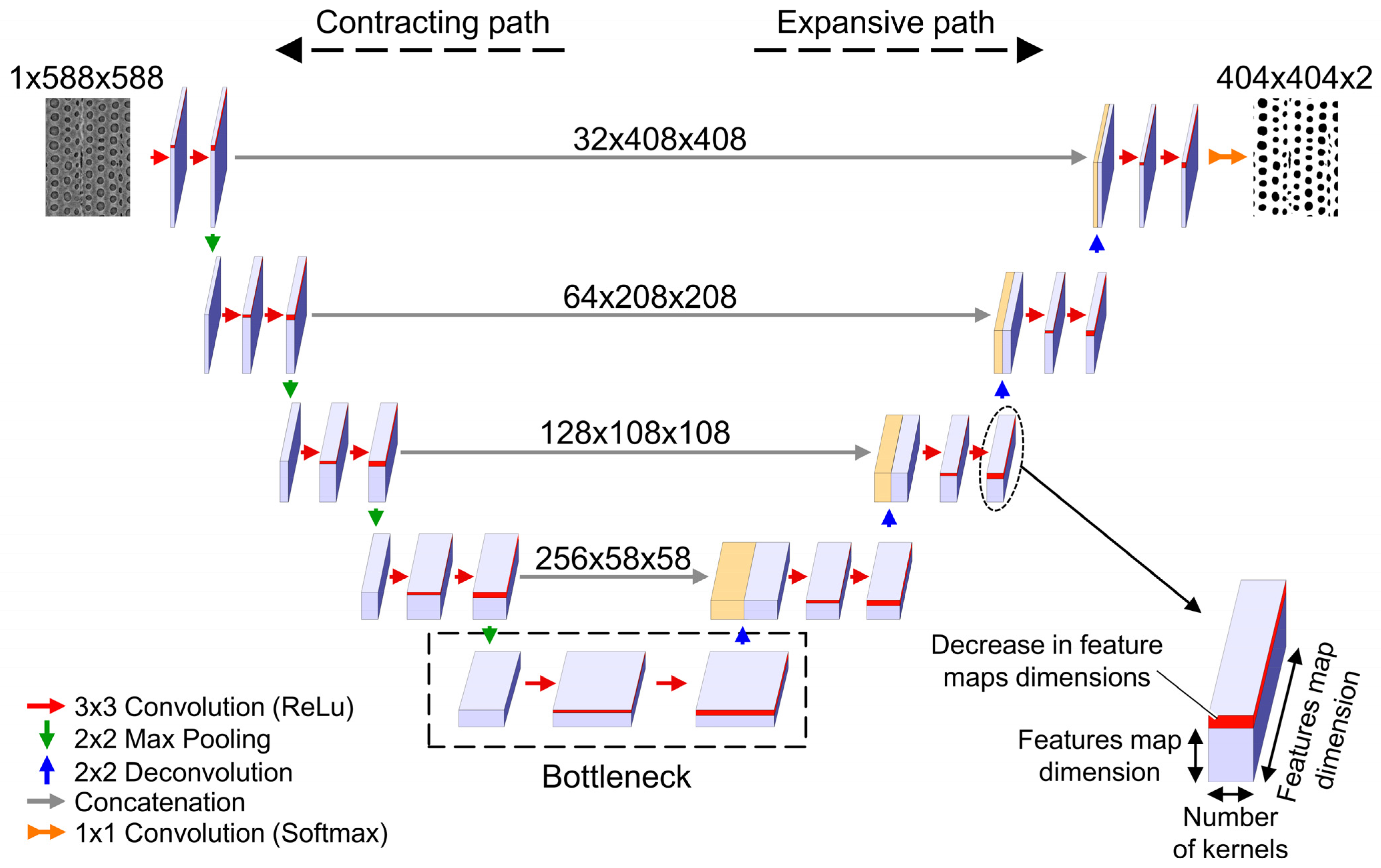
3.2. Convolutional Neural Network (CNN) for Image Segmentation

The CNN used in this work was an adaptation from the U-Net architecture [26]. Initial efforts to use the original U-Net architecture resulted in over-fitting. Over-fitting in machine learning models occurs when the training dataset accuracy is greater than the testing dataset accuracy [39]. For CNNs, over-fitting indicates that the model has more filters than needed [39]. To avoid over-fitting, the total network size was decreased by reducing the number of feature maps calculated in each layer by 50% as compared to the original U-Net architecture, which also reduced the number of weights and biases from 31 million to 7.7 million. This reduction resulted in training and testing datasets with similar levels of accuracy. The modified network retained the identical sequences of layers as U-Net and was composed of a contracting path, a bottleneck, and an expansive path (Figure 5). Each successive layer doubled the number of feature maps in the contracting path but halved the resolution of those feature maps by employing convolution and max-pooling operators. The modified network started with calculating 32 feature maps in the first layer, then increased in each successive layer until reaching a maximum of 512 feature maps at the bottleneck. Conversely, in the expansive path the number of feature maps was halved in each successive layer, but the feature map resolution doubled. This path contained convolution and transposed convolution operations. The U-Net CNN architecture made use of high-resolution and low-resolution feature maps to classify the pixels. High-resolution feature maps helped the network identify the context related to each class, while low-resolution maps helped the network better locate those classes.
For the CNN training and validation, 78 images were randomly chosen from earlywood and latewood samples at different RH to create ground-truth images. A combination of traditional threshold and manual segmentation using ImageJ [37] was used to create ground-truth images. The number of training images was increased by partitioning the ground-truth images into 588 × 588-pixel sub-images and employing data augmentation. The training data augmentation was achieved by rotating each sub-image in five different directions. These operations increased the number of training images from 78 full-size images to 14,010 sub-images with 588 × 588-pixel dimensions. Seventy percent of the total sub-images were used for training, while the remaining 30% were used for the model validation.
The network was trained using a stochastic gradient descent algorithm [40] for a total of 30 iterations. The training algorithm worked by extracting feature maps from the training images using convolution operators and assigning a weight to each. An error was then calculated using the cross-entropy loss function. The weights were adjusted in every iteration to lower the loss value between the predicted result and the ground-truth image. The result of this training was a CNN that took a single-channel gray-scale image with size 588 × 588 pixels and outputted a resulting two-channel CNN image with size of 404 × 404 pixels. The two channels corresponded to the probability of the pixel belonging to the cell wall or air class. Because there are only two classes in this segmentation problem, all the segmentation information is included in one channel and the cell wall probability channel was chosen for further analysis.
Because the CNN output size was smaller than the input size, partitioning the images into overlapping tiles was necessary to offset information loss. The overlap-tile strategy worked by partitioning the full image into multiple overlapping sub-images with dimensions equal to the CNN 588 × 588 pixels input size. The sub-images overlapped sufficiently such that there was no information loss when the smaller 404 × 404 pixels output sub-images were pieced back together. The resulting CNN images were 8-bit grayscale images in which grayscale values corresponded to the probability of being in the cell wall class. Finally, binary images were created by thresholding the CNN image with 0–127 grayscale values assigned to air and 128–255 values assigned to cell wall.
In the absence of reference standards, it is not possible to quantify the accuracy and precision of a segmentation technique. However, an alternative evaluation approach is to use validation metrics for semantic image segmentation that compare ground-truth images with the resulting network segmentation. In this work, the intersection over union (IoU), which is a metric that quantifies the overlap between the classes in the ground-truth image and the network’s resulting binary image [41,42], was used to quantify the accuracy of CNN. For CNN image P and corresponding ground-truth image G, IoU is calculated for each pixel class using the following:
I o U = P G P G ( 100 % )
where P G is the size of the area of overlapping intersection, and P G is the size of the union [42]. IoU ranges from 0 to 100%, with 0% signifying no overlap and 100% signifying perfectly overlapping segmentations.
The network testing data set consisted of the 3034 images reserved from the 14,010 generated ground-truth images. First, the IoU was calculated for both the air and the wood cell wall material classes. The mean IoU for a given image was then calculated by averaging the air and cell wall IoUs. For the full testing data set, an average IoU of 96% was calculated. This means that compared to the ground-truth images, 4% of pixels in the segmented CNN images were misclassified. Compared to the traditional histogram-based segmentation methods tested in the Supplementary Materials, the CNN mean IoU of 96% was much higher with none of the other full image methods reaching 50%. Compared to the literature, this value is also higher than the IoU of 92% reported for the U-Net CNN effectiveness for segmenting the cellular structure of HeLa cells [26]. The 96% IoU also compares favorably to the 73% to 96% IoUs reported for seven different U-net segmentation tasks in biomedical imaging [43].

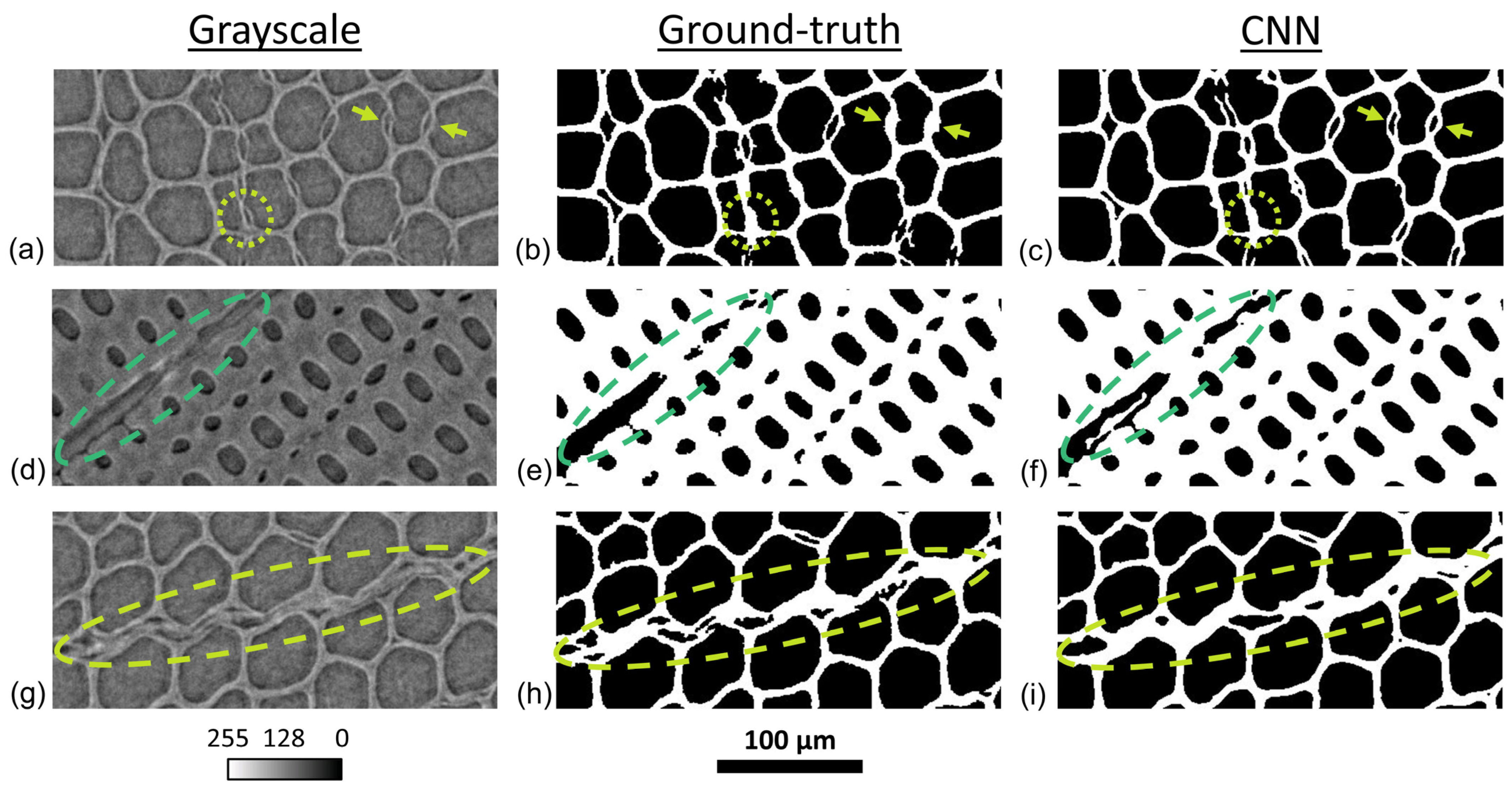
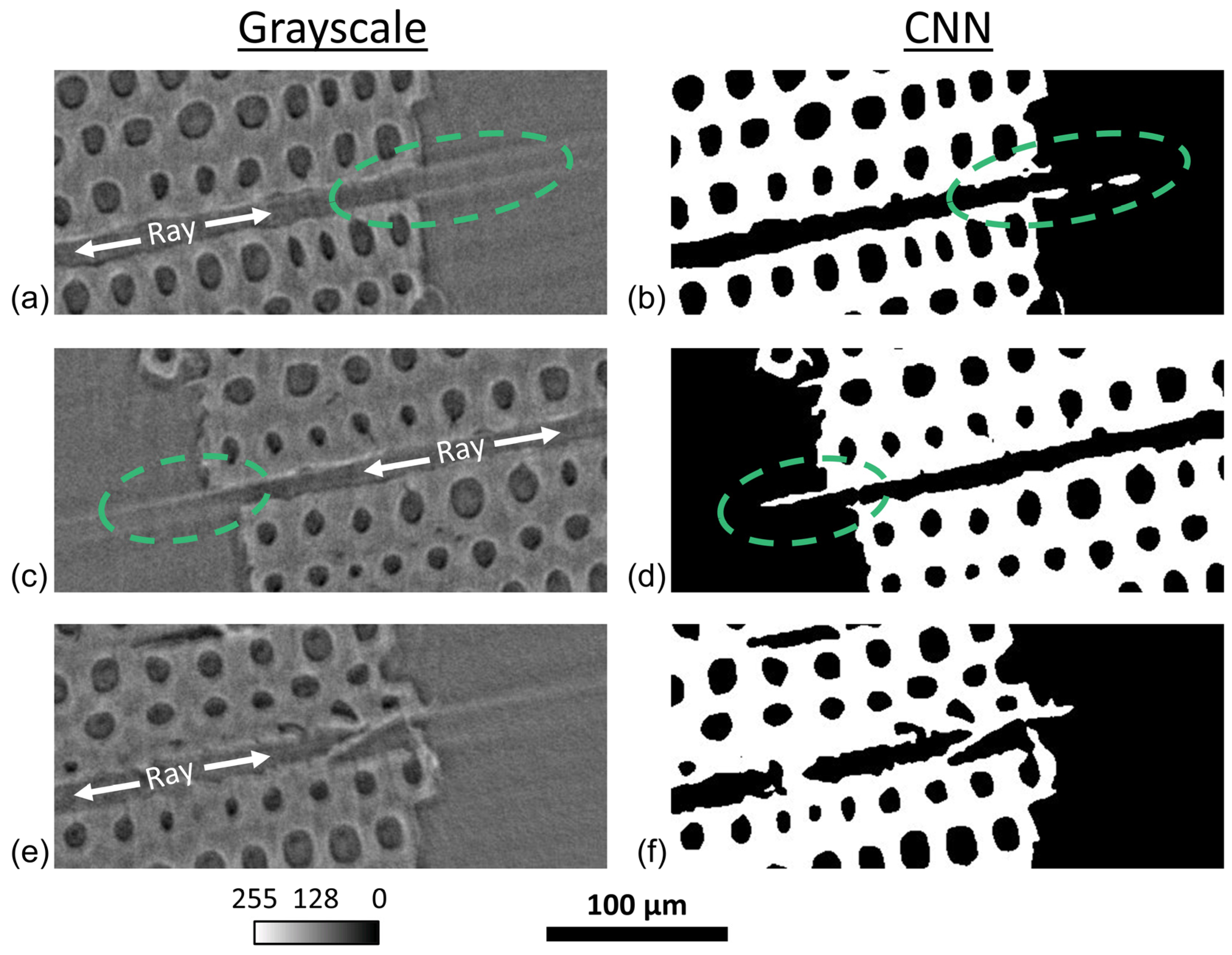
3.3. Qualitative Observations
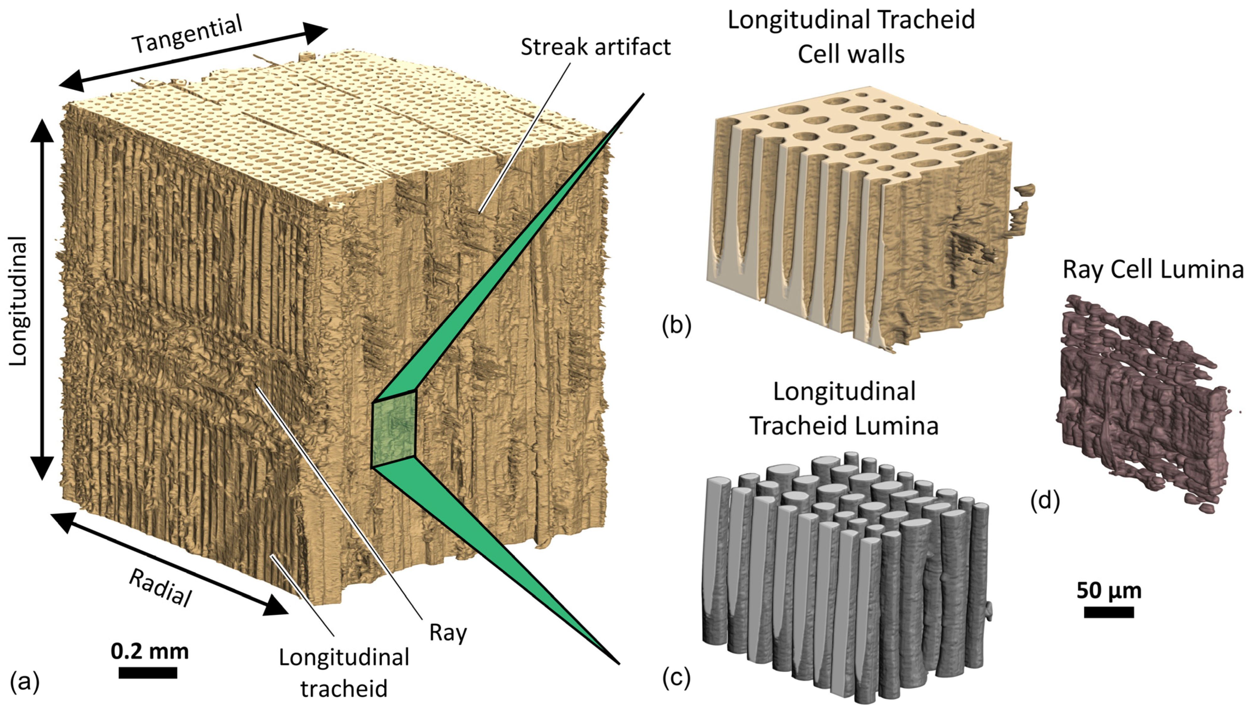
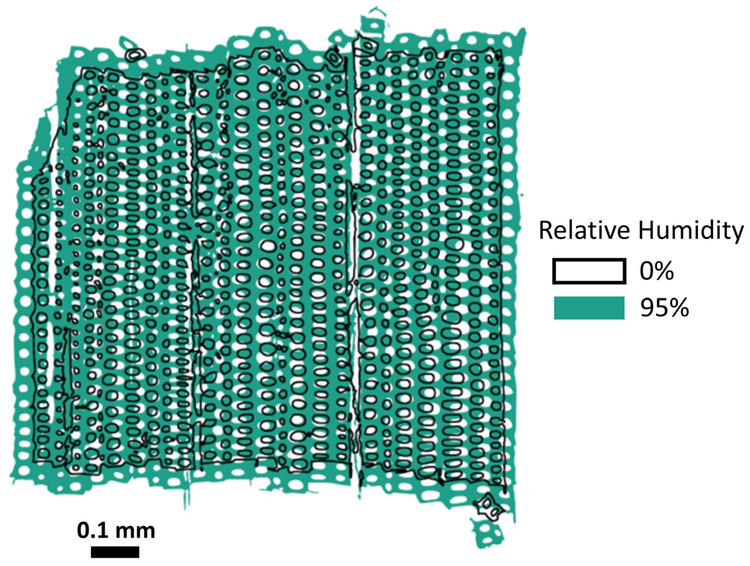
Visual comparisons between reconstructed grayscale, ground-truth binary, and CNN binary images are shown in Figure 6. These close-up images were chosen to highlight a few qualitative observations in the segmented wood cellular structure. Softwood is primarily composed of longitudinal tracheids, whose cross-sections occupy most of the images. The cell walls and lumina in these tracheids are well-defined in the grayscale images and the CNN did well to segment them. Often, the cell wall-lumen interfaces are smoother in the CNN than in the in the ground-truth images, which is more consistent with the grayscale images and suggests the CNN segmentation can outperform manual segmentation. However, some differences between the ground-truth and CNN segmentations were observed in the pits and rays. The arrows in Figure 6a–c show cross sections of two pits that were missed in the manually segmented ground-truth image but were properly segmented by the CNN. The pit in the dotted circle in Figure 6a–c was not properly segmented in the ground-truth nor CNN images. The ray cells, which are indicated by dashed ellipses in Figure 6d–i, are less regularly defined than the longitudinal tracheids in the grayscale images. Even when manually segmenting the ground-truth images some user judgments had to be made with regard to which pixels corresponded to cell wall and air classes in the rays. Although differences were sometimes observed between the ground-truth and CNN segmentations, it was often not possible to unambiguously determine the correct pixel classification. Fortunately, the segmentation uncertainties in pits and rays are not expected to have a substantial effect on the cell wall quantification because most of softwood is composed of tracheids. In loblolly pine, tracheids occupy 96% of the total wood cellular volume and account for 99% of the total cell wall material [44]. Therefore, uncertainties in the segmenting of pits and rays would not be expected to be more than a few percent at most, which is consistent with the quantified CNN mean IoU of 96%.
Streak artifacts caused by the image reconstruction algorithm were also observed to occasionally cause misclassifications in the CNN segmented images. The dashed ellipses in Figure 7a–d show streak artifacts in grayscale images that were partially segmented into the cell wall class in the CNN images. Figure 7e–d shows a similar streak artifact in a grayscale image that was not segmented into the cell wall class. These strong streak artifacts that were sometimes erroneously segmented into the cell wall class were only observed to appear at the edges of wood specimens with large ray cells, such as in the chosen close-ups in Figure 7. As is shown in the next section, streak artifacts that are segmented into the cell wall class affect the three-dimensional visualization of wood specimens. However, the number of pixels in the segmented streak artifacts is very small compared to the number of pixels in the cell wall material. For example, the percentages of pixels in Figure 7b,d that were misclassified in the streak artifact were 0.9% and 0.5%, respectively. Given Figure 7b,d depicts only close-up views of portions of the entire specimen, the actual percentage error would be much smaller and would not be expected to substantially affect cell wall volumes measured from the CNN segmented images.
When inspecting the μXCT image stacks, it was possible to detect that some reconstructed stacks contained blurring noise. After the image segmentation process, it became obvious that the segmented images in these stacks did not correspond to the expected cellular structure. For example, portions of the cell wall material were classified as air or random lumina classified as cell wall, as shown in Figure 8. Also, for a given specimen tested at different RH conditions, the blurring effect was random and only present in scans under certain RH conditions. Therefore, the effect was not specimen dependent. It is likely that this random blurring effect was from lateral vibrations caused by the sample becoming loose in the mounting clay and vibrating during rotations. It is also possible that airflow through the RH chamber caused specimen vibrations. These blurred image stacks will need to be removed in future analyses for calculating moisture swelling because the cell walls cannot be reliably segmented. Future experiments should use mechanical clamping instead of mounting clay to minimize this blurring effect.

3.4. Visualization

Figure 9 shows three-dimensional renderings of a portion of a 1 mm cross-section latewood sample. Like the two-dimensional images, different wood anatomical features can be observed, such as rays and longitudinal tracheids on the exposed radial–longitudinal surface. The small features protruding from the exposed tangential–longitudinal face are streak artifacts and not a real anatomical feature of wood. With stacks of segmented μXCT images, it also possible to virtually separate different components to obtain information about the interior of the sample. For example, Figure 9b–d shows the longitudinal tracheid cell walls, longitudinal tracheid lumina, and ray cell lumina, respectively, from a sub-volume virtually excised from the specimen. In addition to visualization, virtual separations could also be used for quantitative analyses of the different components.
To demonstrate moisture swelling, Figure 10 shows superimposed cross-sectional images at 0% and 95% RH. To better visualize the interior of the sample, the 0% RH image was processed to extract the sample edges. It can be readily observed that the size of the sample cross-section increased as the RH increased. Moreover, it can be observed in the interior of the sample that the width of the rays also increased. Swelling of the cell wall itself is not as easy to observe visually. Fortunately, the cell wall swelling can be easily quantified by using the known 0.65 μm pixel size and summing the number of pixels in the cell wall class at each RH. For this cross-section, the cell wall area increased from 0.49 mm2 to 0.61 mm2 going from 0% to 95% RH. This is an approximately 25% increase. The increase in cell wall swelling is much larger than the estimated errors in the CNN segmentation results, which included from the calculated mean IoU an estimated misclassification of 4% of pixels and qualitative observations of small errors in the CNN segmentation of pits, rays, and streak artifacts. Therefore, CNN segmentation will be adequate to calculate cell wall swelling in wood over this range of RH because the expected amount of swelling is much larger compared to the estimated uncertainties. The 25% increase in cell wall area from the results in Figure 10 was also consistent with previous work. Derome and coworkers also used μXCT to study swelling in latewood Norway spruce cell walls and reported a 12.5% increase in cell wall volume when measured over the smaller RH range of 10% to 85% [13].

4. Conclusions

Fast propagation-based phase-contrast micro-X-ray computed tomography (μXCT) is poised to become a valuable tool to study in situ dynamic processes at the cellular length scales in wood. To overcome the segmentation challenges associated with the decreased grayscale intensity contrast between object classes that occur when materials like wood are imaged with fast μXCT, a modified U-net convolutional neural network (CNN) segmentation method was developed for segmenting wood μXCT images into cell wall and air classes. The efficacy of the new segmentation method was demonstrated in experiments of loblolly pine wood imaged under different RH conditions. The accuracy of the CNN was quantified using the intersection over union (IoU) metric calculated through a comparison of ground-truth binary images to their corresponding CNN binary images. The CNN scored a mean IoU of 96%. Qualitative observations revealed that the small discrepancies between the ground-truth and CNN images primarily arose when segmenting pits, rays, and streak artifacts. Fortunately, these discrepancies represented a very small portion of the wood μXCT images. A few specimens also displayed blurring noise that was likely caused by lateral vibrations during μXCT imaging. The μXCT images with blurring noise could not be reliably segmented and will need to be discarded in future quantitative analyses of this data set. Future μXCT experiments should employ mechanical holders instead of mounting clay to hold specimens more securely and minimize lateral vibrations. Initial observations of moisture swelling in latewood cellular structure revealed that the cell walls swelled about 25% from 0% to 95% RH, and that in the transverse plane ray cell lumina became wider at higher RH. Overall, it was determined that the CNN was sufficient for future quantitative studies of cellular scale processes like moisture swelling in wood cellular structures. The CNN developed here would be expected to perform even better in synthetic cellular materials because synthetic materials lack the pits and rays that cause many of the uncertainties in the CNN segmented wood images.

Supplementary Materials

The following supporting information can be downloaded at: https://www.mdpi.com/article/10.3390/app13148146/s1, Arzola_CNN_SM.pdf. Following are references that appear only in the Supplementary Materials: [45,46,47,48,49,50,51,52,53,54,55,56,57].

Author Contributions

Conceptualization, X.A.-V., J.E.J., R.L. and D.S.S.; methodology, X.A.-V., J.E.J., C.B., J.O., P.S., X.X. and F.D.C.; formal analysis, X.A.-V., J.E.J. and C.B.; data curation, X.A.-V. and J.E.J.; writing—original draft preparation, X.A.-V.; writing—review and editing, J.E.J., C.B., R.L., D.S.S., J.O., P.S., X.X. and F.D.C.; visualization, X.A.-V. and J.E.J.; supervision, J.E.J., R.L. and D.S.S.; funding acquisition, J.E.J., R.L. and D.S.S. All authors have read and agreed to the published version of the manuscript.

Funding

This research used resources of the Advanced Photon Source, a U.S. Department of Energy (DOE) Office of Science user facility operated for the DOE Office of Science by Argonne National Laboratory under Contract No. DE-AC02-06CH11357. Support for X.A was provided by the Graduate Engineering Research Scholars (GERS) program at UW-Madison and USDA Forest Service grants 14-JV-11111129-063, 18-JV-11111129-036, and 22-JV-11111129-029.

Data Availability Statement

Data can be available upon reasonable request to the corresponding author.

Acknowledgments

We acknowledge the machine shop at the Forest Products Laboratory for construction of the in situ relative humidity chambers used in the µXCT experiments. Thank you to Bill Thomas of Shuqualak Lumber for sourcing the Pinus taeda.

Conflicts of Interest

The authors declare no conflict of interest. The funders had no role in the design of the study; in the collection, analyses, or interpretation of data; in the writing of the manuscript; or in the decision to publish the results.

References

  1. Gibson, L.J.; Ashby, M.F. Cellular Solids: Structure and Properties, 2nd ed.; Cambridge University Press: New York, NY, USA, 1997. [Google Scholar]
  2. Jakes, J.E.; Arzola, X.; Bergman, R.; Ciesielski, P.; Hunt, C.G.; Rahbar, N.; Tshabalala, M.; Wiedenhoeft, A.C.; Zelinka, S.L. Not just lumber—Using wood in the sustainable future of materials, chemicals, and fuels. JOM 2016, 68, 2395–2404. [Google Scholar] [CrossRef] [Green Version]
  3. Brandner, R.; Flatscher, G.; Ringhofer, A.; Schickhofer, G.; Thiel, A. Cross laminated timber (CLT): Overview and development. Eur. J. Wood Wood Prod. 2016, 74, 331–351. [Google Scholar] [CrossRef]
  4. Rajendra, S.; Ho, T.X.; Arijit, S. Structural Performance Characterization of Mass Plywood Panels. J. Mater. Civ. Eng. 2021, 33, 4021275. [Google Scholar] [CrossRef]
  5. Hofstetter, K.; Gamstedt, E.K. Hierarchical modelling of microstructural effects on mechanical properties of wood. A review COST Action E35 2004–2008: Wood machining—Micromechanics and fracture. Holzforschung 2009, 63, 130–138. [Google Scholar] [CrossRef]
  6. Salmen, L.; Burgert, I. Cell wall features with regard to mechanical performance. A review. COST Action E35 2004–2008: Wood machining—Micromechanics and fracture. Holzforschung 2009, 63, 121–129. [Google Scholar] [CrossRef]
  7. Glass, S.; Zelinka, S. Moisture relations and physical properties of wood. In Wood Handbook: Wood as an Engineering Material; GTR-190; US Department of Agriculture, Forest Service, Forest Products Laboratory: Madison, WI, USA, 2010; pp. 1–19. [Google Scholar]
  8. Jakes, J.E.; Frihart, C.R.; Hunt, C.G.; Yelle, D.J.; Plaza, N.Z.; Lorenz, L.F.; Ching, D.J. Integrating Multi-Scale Studies of Adhesive Penetration into Wood. For. Prod. J. 2018, 68, 340–348. [Google Scholar]
  9. Arzola-Villegas, X.; Lakes, R.; Plaza, N.Z.; Jakes, J.E. Wood Moisture-Induced Swelling at the Cellular Scale—Ab Intra. Forests 2019, 10, 996. [Google Scholar] [CrossRef] [Green Version]
  10. Wiedenhoeft, A.C. Structure and Function of Wood. In Handbook of Wood Chemistry and Wood Composites; Rowell, R.M., Ed.; CRC Press: Boca Raton, FL, USA, 2013; pp. 9–32. [Google Scholar]
  11. Nikitin, V.; Tekawade, A.; Duchkov, A.; Shevchenko, P.; De Carlo, F. Real-time streaming tomographic reconstruction with on-demand data capturing and 3D zooming to regions of interest. J. Synchrotron Radiat. 2022, 29, 816–828. [Google Scholar] [CrossRef] [PubMed]
  12. Cierniak, R. X-ray Computed Tomography in Biomedical Engineering; Springer Science & Business Media: Heidelberg, Germany, 2011; ISBN 0857290274. [Google Scholar]
  13. Derome, D.; Griffa, M.; Koebel, M.; Carmeliet, J. Hysteretic swelling of wood at cellular scale probed by phase-contrast X-ray tomography. J. Struct. Biol. 2011, 173, 180–190. [Google Scholar] [CrossRef] [PubMed]
  14. Patera, A.; Derome, D.; Griffa, M.; Carmeliet, J. Hysteresis in swelling and in sorption of wood tissue. J. Struct. Biol. 2013, 182, 226–234. [Google Scholar] [CrossRef]
  15. Paris, J.L.; Kamke, F.A. Quantitative wood–adhesive penetration with X-ray computed tomography. Int. J. Adhes. Adhes. 2015, 61, 71–80. [Google Scholar] [CrossRef]
  16. Jakes, J.E.; Frihart, C.R.; Hunt, C.G.; Yelle, D.J.; Plaza, N.Z.; Lorenz, L.; Grigsby, W.; Ching, D.J.; Kamke, F.; Gleber, S.-C.; et al. X-ray methods to observe and quantify adhesive penetration into wood. J. Mater. Sci. 2019, 54, 705–718. [Google Scholar] [CrossRef]
  17. Zhao, J.; Li, L.; Lv, P.; Sun, Z.; Cai, Y. A comprehensive evaluation of axial gas permeability in wood using XCT imaging. Wood Sci. Technol. 2023, 57, 33–50. [Google Scholar] [CrossRef]
  18. McKinley, P.E.; Ching, D.J.; Kamke, F.A.; Zauner, M.; Xiao, X. Micro X-ray Computed Tomography of Adhesive Bonds in Wood. Wood Fiber Sci. 2016, 48, 2–16. [Google Scholar]
  19. Ching, D.J.; Kamke, F.A.; Bay, B.K. Methodology for comparing wood adhesive bond load transfer using digital volume correlation. Wood Sci. Technol. 2018, 52, 1569–1587. [Google Scholar] [CrossRef]
  20. Forsberg, F.; Mooser, R.; Arnold, M.; Hack, E.; Wyss, P. 3D micro-scale deformations of wood in bending: Synchrotron radiation μCT data analyzed with digital volume correlation. J. Struct. Biol. 2008, 164, 255–262. [Google Scholar] [CrossRef]
  21. Zauner, M.; Keunecke, D.; Mokso, R.; Stampanoni, M.; Niemz, P. Synchrotron-based tomographic microscopy (SbTM) of wood: Development of a testing device and observation of plastic deformation of uniaxially compressed Norway spruce samples. Holzforschung 2012, 66, 973–979. [Google Scholar] [CrossRef] [Green Version]
  22. Pare, S.; Kumar, A.; Singh, G.K.; Bajaj, V. Image Segmentation Using Multilevel Thresholding: A Research Review. Iran. J. Sci. Technol. Trans. Electr. Eng. 2020, 44, 1–29. [Google Scholar] [CrossRef]
  23. Born, M.; Wolf, E. Principles of Optics: Electromagnetic Theory of Propagation, Interference and Diffraction of Light, 6th ed.; Pergamon Press: New York, NY, USA, 1980; ISBN 148310320X. [Google Scholar]
  24. Paris, J.L.; Kamke, F.A.; Xiao, X. X-ray computed tomography of wood-adhesive bondlines: Attenuation and phase-contrast effects. Wood Sci. Technol. 2015, 49, 1185–1208. [Google Scholar] [CrossRef]
  25. Galvez-Hernandez, P.; Gaska, K.; Kratz, J. Phase segmentation of uncured prepreg X-Ray CT micrographs. Compos. Part A Appl. Sci. Manuf. 2021, 149, 106527. [Google Scholar] [CrossRef]
  26. Ronneberger, O.; Fischer, P.; Brox, T. U-Net: Convolutional Networks for Biomedical Image Segmentation BT—Medical Image Computing and Computer-Assisted Intervention—MICCAI 2015; Navab, N., Hornegger, J., Wells, W.M., Frangi, A.F., Eds.; Springer International Publishing: Cham, Switzerland, 2015; pp. 234–241. [Google Scholar]
  27. Liu, X.; Deng, Z.; Yang, Y. Recent progress in semantic image segmentation. Artif. Intell. Rev. 2019, 52, 1089–1106. [Google Scholar] [CrossRef] [Green Version]
  28. Teuwen, J.; Moriakov, N. Chapter 20—Convolutional neural networks. In The Elsevier and MICCAI Society Book Series; Zhou, S.K., Rueckert, D., Fichtinger, G., Eds.; Academic Press: Cambridge, MA, USA, 2020; pp. 481–501. ISBN 978-0-12-816176-0. [Google Scholar]
  29. Ajit, A.; Acharya, K.; Samanta, A. A Review of Convolutional Neural Networks. In Proceedings of the 2020 International Conference on Emerging Trends in Information Technology and Engineering (ic-ETITE), Vellore, India, 24–25 February 2020; pp. 1–5. [Google Scholar]
  30. Wang, Y.; De Carlo, F.; Foster, I.; Insley, J.; Kesselman, C.; Lane, P.; von Laszewski, G.; Mancini, D.C.; McNulty, I.; Su, M.-H.; et al. Quasi-real-time x-ray microtomography system at the Advanced Photon Source. In Proceedings of the SPIE’s International Symposium on Optical Science, Engineering, and Instrumentation, Denver, CO, USA, 18–23 July 1999; Volume 3772, pp. 318–327. [Google Scholar]
  31. De Carlo, F.; Albee, P.B.; Chu, Y.S.; Mancini, D.C.; Tieman, B.; Wang, S.Y. High-throughput real-time x-ray microtomography at the Advanced Photon Source. In Proceedings of the SPIE International Symposium on Optical Science and Technology, San Diego, CA, USA, 29 July–3 August 2001; Volume 4503, pp. 1–13. [Google Scholar]
  32. Greenspan, L. Humidity fixed points of binary saturated aqueous solutions. J. Res. Natl. Bur. Stand. Sect. A Phys. Chem. 1977, 81, 89. [Google Scholar] [CrossRef]
  33. Gürsoy, D.; De Carlo, F.; Xiao, X.; Jacobsen, C. TomoPy: A framework for the analysis of synchrotron tomographic data. J. Synchrotron Radiat. 2014, 21, 1188–1193. [Google Scholar] [CrossRef] [Green Version]
  34. Münch, B.; Trtik, P.; Marone, F.; Stampanoni, M. Stripe and ring artifact removal with combined wavelet—Fourier filtering. Opt. Express 2009, 17, 8567–8591. [Google Scholar] [CrossRef] [Green Version]
  35. Rivers, M.L. tomoRecon: High-speed tomography reconstruction on workstations using multi-threading. In Proceedings of the SPIE Optical Engineering + Applications, San Diego, CA, USA, 12–16 August 2012; Volume 8506, p. 85060U. [Google Scholar]
  36. Kohno, H.; Tanji, Y.; Fujimoto, K.; Kitajima, H.; Horikawa, Y.; Takahashi, N. Reconstruction of CT images using iterative least-squares methods with nonnegative constraint. J. Signal Process. 2019, 23, 41–48. [Google Scholar] [CrossRef]
  37. Schneider, C.A.; Rasband, W.S.; Eliceiri, K.W. NIH Image to ImageJ: 25 years of image analysis. Nat. Methods 2012, 9, 671–675. [Google Scholar] [CrossRef]
  38. Van Rossum, G.; Drake, F.L., Jr. Python Reference Manual; Centrum Voor Wiskunde en Informatica: Amsterdam, The Netherlands, 1994. [Google Scholar]
  39. Michelucci, U. Advanced Applied Deep Learning: Convolutional Neural Networks and Object Detection; Springer: Berlin/Heidelberg, Germany, 2019; ISBN 1484249763. [Google Scholar]
  40. Rumelhart, D.E.; Hinton, G.E.; Williams, R.J. Learning representations by back-propagating errors. Nature 1986, 323, 533–536. [Google Scholar] [CrossRef]
  41. Jaccard, P. The Distribution of the Flora in the Alpine Zone.1. New Phytol. 1912, 11, 37–50. [Google Scholar] [CrossRef]
  42. Rahman, M.A.; Wang, Y. Optimizing Intersection-Over-Union in Deep Neural Networks for Image Segmentation BT—Advances in Visual Computing; Bebis, G., Boyle, R., Parvin, B., Koracin, D., Porikli, F., Skaff, S., Entezari, A., Min, J., Iwai, D., Sadagic, A., et al., Eds.; Springer International Publishing: Cham, Switzerland, 2016; pp. 234–244. [Google Scholar]
  43. Yin, X.-X.; Sun, L.; Fu, Y.; Lu, R.; Zhang, Y. U-Net-Based Medical Image Segmentation. J. Healthc. Eng. 2022, 2022, 4189781. [Google Scholar] [CrossRef]
  44. Onilude, M.A. Quantitative Anatomical Characteristics of Plantation Grown Loblolly Pine (Pinus taeda L.) and Cottonwood (Populus Deltoides Bart. ex Marsh) and Their Relationships to Mechanical Properties. Ph.D. Thesis, Virginia Polytechnic Institute and State University, Blacksburg, VA, USA, 1982. [Google Scholar]
  45. Huang, L.-K.; Wang, M.-J.J. Image thresholding by minimizing the measures of fuzziness. Pattern Recognit. 1995, 28, 41–51. [Google Scholar] [CrossRef]
  46. Prewitt, J.M.S.; Mendelsohn, M.L. The analysis of cell images. Ann. N. Y. Acad. Sci. 1966, 128, 1035–1053. [Google Scholar] [CrossRef]
  47. Shanbhag, A.G. Utilization of Information Measure as a Means of Image Thresholding. CVGIP Graph. Model. Image Process. 1994, 56, 414–419. [Google Scholar] [CrossRef]
  48. Zack, G.W.; Rogers, W.E.; Latt, S.A. Automatic measurement of sister chromatid exchange frequency. J. Histochem. Cytochem. 1977, 25, 741–753. [Google Scholar] [CrossRef] [PubMed]
  49. Yen, J.-C.; Chang, F.-J.; Chang, S. A new criterion for automatic multilevel thresholding. IEEE Trans. Image Process. 1995, 4, 370–378. [Google Scholar] [CrossRef] [PubMed]
  50. Ridler, T.W.; Calvard, S. Picture Thresholding Using an Iterative Selection Method. IEEE Trans. Syst. Man. Cybern. 1978, 8, 630–632. [Google Scholar] [CrossRef]
  51. Li, C.H.; Lee, C.K. Minimum cross entropy thresholding. Pattern Recognit. 1993, 26, 617–625. [Google Scholar] [CrossRef]
  52. Kapur, J.N.; Sahoo, P.K.; Wong, A.K.C. A new method for gray-level picture thresholding using the entropy of the histogram. Comput. Vision Graph. Image Process. 1985, 29, 273–285. [Google Scholar] [CrossRef]
  53. Glasbey, C.A. An Analysis of Histogram-Based Thresholding Algorithms. CVGIP Graph. Model. Image Process. 1993, 55, 532–537. [Google Scholar] [CrossRef]
  54. Kittler, J.; Illingworth, J. Minimum error thresholding. Pattern Recognit. 1986, 19, 41–47. [Google Scholar] [CrossRef]
  55. Tsai, W.-H. Moment-preserving thresolding: A new approach. Comput. Vision, Graph. Image Process. 1985, 29, 377–393. [Google Scholar] [CrossRef]
  56. Otsu, N. A threshold selection method from gray-level histograms. IEEE Trans. Syst. Man. Cybern. 1979, 9, 62–66. [Google Scholar] [CrossRef] [Green Version]
  57. Doyle, W. Operations useful for similarity-invariant pattern recognition. J. ACM 1962, 9, 259–267. [Google Scholar] [CrossRef]
Figure 1. Illustration of softwood cellular structure. Softwood is an anisotropic cellular material defined by the radial, tangential, and longitudinal directions [10]. It is mainly composed of longitudinal tracheids and ray cells. Pits are small openings between cells that facilitate intercellular water transport. A single longitudinal tracheid can be thought of as a hollow tube with the open space called a lumen. The cell wall is a multilamellar structure with secondary cell wall layers that are nanofiber-reinforced composites consisting of helically wound cellulose microfibrils embedded in a matrix of amorphous cellulose, hemicelluloses, and lignin [6]. Wood polymers are hygroscopic, and as a hygroscopic material wood’s properties and performance depend on the amount of water in the wood [7]. Growth rings consist of earlywood and latewood layers. Latewood is denser than earlywood because its tracheids have smaller lumina and thicker cell walls.
Applsci 13 08146 g001
Figure 2. Custom-built relative humidity (RH) chamber for APS beamline 2-BM-B. The chamber separated into two pieces to facilitate sample changes. The top of the chamber consisted of 6.3 cm length of a Precision Paper Tube Company (Wheeling, IL, USA) Kapton© tube with 127 µm thick walls and 4.45 cm outside diameter. The Kapton© tube had machined aluminum caps at each end. The bottom consisted of machined aluminum with a Ted Pella™ (Mountain Lakes Blvd, Redding, CA, USA) pin mount sample holder that was secured in the chamber with a set screw, a hose barb connector for the RH generator connection, a Sensirion™ (Staefa, Switzerland) SHT1x relative humidity and temperature sensor to monitor the conditions inside the chamber, and a ThorLabs™ (Sparta Ave, Newton, NJ, USA) kinematic mount to attach the RH chamber to the beamline rotation stage.
Applsci 13 08146 g002
Figure 3. Comparison between the (a) filtered back projection (FBP) and the (b) conjugate gradient least squares (CGLS) reconstruction algorithms. The images are 8-bit and no filters were applied post-reconstruction. The line profiles show the noise along the white lines for each algorithm with regions of void and cell walls indicated with v and c, respectively. Intensity bar has units of grayscale values.
Applsci 13 08146 g003
Figure 4. Representative 8-bit reconstruction slices from 1 mm cross-section (a) latewood and (b) earlywood specimens with their corresponding histograms in (c) and (d), respectively. The close-up views in (e) and (f) are from the white boxes in (a) and (b), respectively. Intensity bars have units of grayscale values.
Applsci 13 08146 g004
Figure 5. Convolutional neural network (CNN) architecture diagram used in this work. This CNN was an adaptation from the U-Net architecture designed by Ronneberger and coworkers [26].
Applsci 13 08146 g005
Figure 6. Comparison of (a,d,g) grayscale, (b,e,h) ground-truth binary, and (c,f,i) convolutional neural network (CNN) binary images. The grayscale images are 8-bit with no filters applied post-reconstruction. Intensity bar has units of grayscale values.
Applsci 13 08146 g006
Figure 7. Comparisons of (a,c,e) grayscale and (b,d,f) convolutional neural networks (CNN) binary images showing streak artifacts. The grayscale images are 8-bit with no filters applied post-reconstruction. Intensity bar has units of grayscale values.
Applsci 13 08146 g007
Figure 8. Comparison of (a)grayscale and (b) convolutional neural network (CNN) binary images showing the effects of blurring noise in a 0.5 mm cross-section latewood specimen. The grayscale images are 8-bit with no filters applied post-reconstruction. Intensity bar has units of grayscale values.
Applsci 13 08146 g008
Figure 9. Three-dimensional renderings from a 1 mm cross-section latewood specimen conditioned at 0% relative humidity. The full image (a) is from 1400 image slices corresponding to a total length of 910 μm. The sub volumes show virtually separated (b) longitudinal tracheid cell walls, (c) longitudinal tracheid lumina, and (d) ray cell lumina.
Applsci 13 08146 g009
Figure 10. Superimposed 1 mm cross-sections of a latewood sample conditioned at 0% and 95% relative humidity.
Applsci 13 08146 g010
Table 1. Desiccant or salts used in saturated aqueous solutions with corresponding relative humidity condition created [32].
Relative Humidity
Desiccant0%
Magnesium chloride33%
Sodium chloride75%
Potassium chloride95%
Disclaimer/Publisher’s Note: The statements, opinions and data contained in all publications are solely those of the individual author(s) and contributor(s) and not of MDPI and/or the editor(s). MDPI and/or the editor(s) disclaim responsibility for any injury to people or property resulting from any ideas, methods, instructions or products referred to in the content.

