Generalized Function Projective Synchronization of Two Different Chaotic Systems with Uncertain Parameters

Abstract

This study proposes a new approach to realize generalized function projective synchronization (GFPS) between two different chaotic systems with uncertain parameters. The GFPS condition is derived by converting the differential equations describing the synchronization error systems into a series of Volterra integral equations on the basis of the Laplace transform method and convolution theorem, which are solved by applying the successive approximation method in the theory of integral equations. Compared with the results obtained by constructing Lyapunov functions or calculating the conditional Lyapunov exponents, the uncertain parameters and the scaling function factors considered in this paper have fewer restrictions, and the parameter update laws designed for the estimation of the uncertain parameters are simpler and easier to realize physically.

1. Introduction

Since Pecora and Carroll realized synchronization between two chaotic systems in 1990 [1,2], chaos synchronization has been widely explored and studied due to its potential applications in vast areas of physics and engineering science [3,4,5,6]. Synchronization is a process wherein two or more systems adjust a given property of their motion. Different types of synchronization phenomena have been numerically observed and experimentally verified in a variety of chaotic systems, such as complete synchronization [1,7], phase synchronization [8,9], anti-phase synchronization [10,11], lag synchronization [12,13], generalized synchronization [14,15] and projective synchronization [16,17].

Complete synchronization (CS) is characterized by a coincidence of states of two chaotic systems while evolving in time. CS only appears when two interacting systems are identical. However, it is difficult to construct two absolutely identical systems in the real world. Generalized synchronization (GS) refers to a functional relation of states of two different chaotic systems, which is an extension of CS. Projective synchronization (PS) is more complex than CS but simpler than GS. Additionally, PS is useful in extending binary digital to M-nary digital communication to achieve faster communication [18,19,20].

PS was first reported by Mainieri et al. [16] in a class of systems with partial linearity in which the drive and response vectors evolve in a proportional scale. Xu [21] showed that the scaling factor of PS in coupled partially linear systems is unpredictable and can be arbitrarily maneuvered by introducing a feedback control to master systems. The PS between two chaotic discrete dynamical systems was achieved by Xin and Wu [22] via linear state error feedback control. Wen and Xu [23] and Yan and Li [24] extended the projective synchronization feature to general nonlinear systems, including non-partially linear chaotic systems, by applying controllers to response systems, which is called generalized projective synchronization (GPS) and was studied later [25,26,27]. CS and anti-synchronization are particular cases of GPS. As an extension of GPS, modified projective synchronization (MPS) was introduced by Li et al. [28] and He et al. [29], where the responses of synchronized dynamical states can be synchronized up to a constant matrix. The combined projective synchronization (CPS) among different nonlinear systems has been reported by Feng et al. [30] by means of the active backstepping design method. Chen et al. [31,32] considered two chaotic systems synchronized up to a scaling function factor, which is called function projective synchronization (FPS). The FPS between two novel chaotic systems has been investigated by El Dessoky et al. [33] and Bekiros et al. [34] using the Lyapunov method of stability. Du et al. [35] and Srisuntorn et al. [36] discussed modified function projective synchronization (MFPS), in which two chaotic systems can be synchronized up to a desired scaling function matrix. As another extension of MPS and FPS, in generalized function projective synchronization (GFPS), the scaling function matrix is more generalized than that of MFPS, as has been discussed by Yu and Li [37], Li and Zhao [38], Wu et al. [39] and Al-Azzawi [40].

Most of the previous works have focused on the constant scaling factor and mainly on chaotic systems with exactly known parameters. However, in many practical situations, GFPS needs to be investigated while some parameters are uncertain. It is easy to understand that GFPS may be greatly affected by these uncertainties. Yu and Li [37] designed an adaptive controller to achieve GFPS between two different chaotic systems and gain some parameter update laws to estimate the unknown parameters of chaotic systems. Li and Zhao [38] firstly discussed the GFPS conditions of two different uncertain hyperchaotic systems when the scaling function factors were periodic functions and polynomial functions. However, only a few theoretical results about GFPS between two different uncertain chaotic systems have been obtained [41,42,43,44,45]. Furthermore, the aforementioned controllers all are designed through the construction of proper Lyapunov functions. The added controllers therefore are often very specific and may be too difficult to realize physically.

In this paper, an effective approach is proposed to design an adaptive controller to realize GFPS between two different uncertain chaotic systems. Moreover, the unknown parameters in the coupled system can be estimated by given parameter update laws. The key to realizing GFPS between two chaotic systems is the determination of the stability of the synchronization error system. In previous works, this problem usually was solved by using the Lyapunov method. However, there are two main difficulties in this method: the first one is that it is challenging to construct a proper Lyapunov function; the second is that the GFPS conditions derived using the Lyapunov method are usually sufficient and highly conserved. The controllers and parameter update laws designed based on such conditions are often very specific. In fact, GFPS can be viewed as a unique case of GS, which can be investigated using the auxiliary system approach [46]. To avoid the construction of Lyapunov functions, the approach presented in this paper converts the differential equations describing the synchronization error system between the auxiliary system and the response system into a series of Volterra integral equations by using the Laplace transform method. Then, the dynamical behavior of the error system near its origin can be analyzed by employing the successive approximation method [47]. In the theory of integral equations, the significance of the Laplace transform method is that the GFPS condition can be obtained without the construction of Lyapunov functions, even if the scaling function factors are periodic functions, polynomial functions or any other complex functions. Compared to previous works, our approach allows the easier design of controllers and simpler parameter update laws and removes some restrictions on the uncertain parameters. The feasibility and effectiveness of the approach are illustrated by several numerical simulations.

The rest of the paper is organized as follows. In Section 2, the GFPS scheme for two different uncertain chaotic systems is introduced. In Section 3, the GFPS condition is investigated using the Laplace transform method combined with the successive approximation method in the theory of Volterra integral equations. A numerical example is provided in Section 4 to demonstrate the effectiveness of our GFPS scheme. In Section 5, simple parameter update laws are designed according to the GFPS condition derived in Section 3 to estimate the uncertain parameters in chaotic systems, the validity of which are illustrated by numerical simulations. Finally, conclusions are drawn in Section 6.

2. GFPS Scheme between Two Different Uncertain Chaotic Systems

Consider two chaotic systems (drive–response systems) with uncertain parameters given in the following form:

$$\begin{array}{cc}\hfill & \dot{x}=f_1(x,\varphi ),\hfill \\ \hfill & \dot{y}=f_2(y,\psi )+u,\hfill \end{array}$$

(1)

where $x,y\in R^n$; $\varphi \in R^m,\psi \in R^l$ are uncertain parameter vectors, and u is the controller to be designed. For simplicity, assume that $f_1(0,\varphi )=f_2(0,\psi )=0$ hold for any values of $\varphi$ and $\psi$. If there exists a scaling function matrix $h=diag\{h_1\left(x\right),$$h_2\left(x\right)$$,\cdots$$,h_n\left(x\right)\}$, such that

$$\underset{t\to \infty }{lim}\left|\right|y-h\left(x\right)x\left|\right|=0,$$

(2)

then the two chaotic systems in system (1) are said to be GFPS with respect to the scaling function matrix h [37,40]. The two chaotic systems are said to be FPS if

$$h_1\left(x\right)=h_2\left(x\right)=\cdots =h_n\left(x\right)$$

in Equation (2). Moreover, we find MPS between the two chaotic systems if $h=diag\{h_1,$$h_2,$$\cdots ,$$h_n\},$ $h_i$($i=1,2,\cdots ,n$) are real constants in Equation (2). Obviously, both FPS and MPS are specific cases of GFPS.

The controller u and the parameter update laws in system (1) are designed as below:

$$\begin{array}{cc}\hfill & u=J\left(x\right)f_1(x,\widehat{\varphi })-f_2(y,\widehat{\psi })+k{\delta }_1,\hfill \\ \hfill & \dot{\widehat{\varphi }}=g_1(\widehat{\varphi }-\varphi ,{\delta }_1),\hfill \\ \hfill & \dot{\widehat{\psi }}=g_2(\widehat{\psi }-\psi ,{\delta }_1),\hfill \end{array}$$

(3)

where $J\left(x\right)=d\left(h\right(x\left)x\right)/dx$, k is the control parameter, and ${\delta }_1=y-h\left(x\right)x$ is the synchronization error; $\widehat{\varphi }$ and $\widehat{\psi }$ are the estimated values of uncertain parameter vectors $\varphi$ and $\psi$, respectively. In addition, $g_1(\widehat{\varphi }-\varphi ,0)=g_2(\widehat{\psi }-\psi ,0)=0$ hold if

$$\widehat{\varphi }=\varphi and\widehat{\psi }=\psi .$$

(4)

The GFPS occurring in system (1) can be regarded as a specific case of GS between the two chaotic systems, which can be detected using the auxiliary system approach [46]. Consider the following identical copy of the response system driven by the same driving signal x,

$$\begin{array}{cc}\hfill & \dot{z}=f_2(z,\psi )+\overline{u},\hfill \\ \hfill & \overline{u}=J\left(x\right)f_1(x,\overline{\varphi })-f_2(z,\overline{\psi })+k{\delta }_2,\hfill \\ \hfill & \dot{\overline{\varphi }}=g_1(\overline{\varphi }-\varphi ,{\delta }_2),\hfill \\ \hfill & \dot{\overline{\psi }}=g_2(\overline{\psi }-\psi ,{\delta }_2),\hfill \end{array}$$

(5)

in which $z\in R^n$ and ${\delta }_2=z-h\left(x\right)x$. $\overline{\varphi }$ and $\overline{\psi }$ are the estimated values of uncertain parameter vectors $\varphi$ and $\psi$, respectively. Additionally, $g_1(\overline{\varphi }-\varphi ,0)=g_2(\overline{\psi }-\psi ,0)=0$ hold for

$$\overline{\varphi }=\varphi and\overline{\psi }=\psi .$$

(6)

Then, GFPS conditions (2) and (4) lead to

$$\underset{t\to \infty }{lim}\left|\right|y-z\left|\right|=0,\underset{t\to \infty }{lim}\left|\right|\widehat{\varphi }-\overline{\varphi }\left|\right|=0,\underset{t\to \infty }{lim}\left|\right|\widehat{\psi }-\overline{\psi }\left|\right|=0.$$

(7)

3. Detection of GFPS Condition Based on the Laplace Transform

By letting

$$\begin{array}{cc}\hfill & e_1=\frac{y-z}{2},e_2=\frac{\widehat{\varphi }-\overline{\varphi }}{2},e_3=\frac{\widehat{\psi }-\overline{\psi }}{2}\hfill \\ \hfill & e_4=\frac{y+z}{2},e_5=\frac{\widehat{\varphi }+\overline{\varphi }}{2},e_6=\frac{\widehat{\psi }+\overline{\psi }}{2}\hfill \end{array}$$

systems (1), (3) and (5) become

$$\begin{array}{cc}\hfill & {\dot{e}}_1=k{e}_1+\frac{J\left(x\right)}{2}[f_1(x,e_2+e_5)-f_1(x,e_5-e_2)]+\frac{1}{2}[f_2(e_1+e_4,\psi )-f_2(e_4-e_1,\psi )]\hfill \\ \hfill & +\frac{1}{2}[f_2(e_4-e_1,e_6-e_3)-f_2(e_4+e_1,e_6+e_3)],\hfill \\ \hfill & {\dot{e}}_2=\frac{1}{2}[g_1(e_2+e_5-\varphi ,e_1+e_4-h\left(x\right)x)-g_1(e_5-e_2-\varphi ,e_4-e_1-h\left(x\right)x)],\hfill \\ \hfill & {\dot{e}}_3=\frac{1}{2}[g_2(e_3+e_6-\psi ,e_1+e_4-h\left(x\right)x)-g_2(e_6-e_3-\psi ,e_4-e_1-h\left(x\right)x)],\hfill \\ \hfill & {\dot{e}}_4=k{e}_4+\frac{J}{2}[f_1(x,e_2+e_5)+f_1(x,e_5-e_2)]+\frac{1}{2}[f_2(e_1+e_4,\psi )+f_2(e_4-e_1,\psi )]\hfill \\ \hfill & -\frac{1}{2}[f_2(e_4-e_1,e_6-e_3)+f_2(e_4+e_1,e_6+e_3)],\hfill \\ \hfill & {\dot{e}}_5=\frac{1}{2}[g_1(e_2+e_5-\varphi ,e_1+e_4-h\left(x\right)x)+g_1(e_5-e_2-\varphi ,e_4-e_1-h\left(x\right)x)],\hfill \\ \hfill & {\dot{e}}_6=\frac{1}{2}[g_2(e_3+e_6-\psi ,e_1+e_4-h\left(x\right)x)+g_2(e_6-e_3-\psi ,e_4-e_1-h\left(x\right)x)],\hfill \\ \hfill & \dot{x}=f_1(x,\varphi ).\hfill \end{array}$$

(8)

GFPS condition (7) can be written as

$$\underset{t\to \infty }{lim}\left|\right|e_i\left|\right|=0,i=1,2,3.$$

(9)

For sufficiently small $e_{1,2,3}$ near $(0,0,0)$, the right-hand side of the first three equations in system (8) can be expanded as

$$\begin{array}{cc}\hfill & {\dot{e}}_1=k{e}_1+F_1(x,e_2,e_3),\hfill \\ \hfill & {\dot{e}}_2={\alpha }_1{e}_1+{\alpha }_2{e}_2+F_2(e_1,e_2),\hfill \\ \hfill & {\dot{e}}_3={\alpha }_3{e}_1+{\alpha }_4{e}_3+F_3(e_1,e_3).\hfill \end{array}$$

(10)

where

$$\begin{array}{cc}\hfill & F_1(x,e_2,e_3)=J\left(x\right)\sum _{n=1}^{\infty }\frac{1}{(2n-1)!}\frac{{\partial }^{(2n-1)}{f}_1(x,\varphi )}{\partial {\varphi }^{(2n-1)}}{e}_2^{(2n-1)}-\sum _{n=1}^{\infty }\frac{1}{(2n-1)!}\frac{{\partial }^{(2n-1)}{f}_2(h\left(x\right)x,\psi )}{\partial {\psi }^{(2n-1)}}{e}_3^{(2n-1)},\hfill \\ \hfill & F_2(e_1,e_2)=\sum _{n=1}^{\infty }\frac{1}{(2n+1)!}[\frac{{\partial }^{(2n+1)}{g}_1(0,0)}{\partial {\delta }_1^{(2n+1)}}{e}_1^{(2n+1)}+\frac{{\partial }^{(2n+1)}{g}_1(0,0)}{\partial {(\widehat{\varphi }-\varphi )}^{(2n+1)}}{e}_2^{(2n+1)}],\hfill \\ \hfill & F_3(e_1,e_3)=\sum _{n=1}^{\infty }\frac{1}{(2n+1)!}[\frac{{\partial }^{(2n+1)}{g}_2(0,0)}{\partial {\delta }_1^{(2n+1)}}{e}_1^{(2n+1)}+\frac{{\partial }^{(2n+1)}{g}_2(0,0)}{\partial {(\widehat{\psi }-\psi )}^{(2n+1)}}{e}_3^{(2n+1)}],\hfill \\ \hfill & {\alpha }_1=\frac{\partial g_1(0,0)}{\partial {\delta }_1},{\alpha }_2=\frac{\partial g_1(0,0)}{\partial (\widehat{\varphi }-\varphi )},{\alpha }_3=\frac{\partial g_2(0,0)}{\partial {\delta }_1},{\alpha }_4=\frac{\partial g_2(0,0)}{\partial (\widehat{\psi }-\psi )}.\hfill \end{array}$$

Consider the Laplace transform, defined as follows:

$$\begin{array}{cc}\hfill & E_j\left(s\right)=L[e_j]={\int }_0^{+\infty }{e}_j\left(t\right)e^{-st}dt,\hfill \\ \hfill & e_j\left(t\right)=L^{-1}[E_j]=\frac{1}{2\pi i}{\int }_{\sigma -i\infty }^{\sigma +i\infty }{E}_j\left(s\right)e^{st}ds,j=1,2,3.\hfill \end{array}$$

(11)

Both $e_j$ and $E_j$ are vectors with the same dimensions for $j=1,2,3$. Taking the Laplace transform of $e_{1,2,3}$ on both sides of system (10) yields

$$(S-M){[E_1,E_2,E_3]}^T={[e_{10},e_{20},e_{30}]}^T+{[{\widehat{F}}_1,{\widehat{F}}_2,{\widehat{F}}_3]}^T,$$

(12)

where

$$S=\left[\begin{array}{ccc}s{I}_n& 0& 0\\ 0& s{I}_m& 0\\ 0& 0& s{I}_l\end{array}\right],M=\left[\begin{array}{ccc}k{I}_n& 0& 0\\ {\alpha }_1& {\alpha }_2& 0\\ {\alpha }_3& 0& {\alpha }_4\end{array}\right],$$

(13)

$I_n$, $I_m$, $I_l$ represent the $n\times n$, $m\times m$ and $l\times l$ real identity matrices, respectively. T denotes the transpose of vectors. $e_{j0}$, $j=1,2,3$, are given initial values of system (10) and ${\widehat{F}}_{1,2,3}$ are the Laplace transforms of $F_{1,2,3}$, respectively, i.e.,

$${\widehat{F}}_j=L[F_j]={\int }_0^{+\infty }{F}_j\left(t\right)e^{-st}dt,j=1,2,3.$$

The solution to Equation (12) can be derived by using Cramer’s rule [48]. Take, for example, the expression of $E_1$, which is an n-dimensional vector and always can be given by the form below:

$$E_1=\left[\begin{array}{c}{E}_{11}\\ E_{12}\\ ⋮\\ E_{1n}\end{array}\right]=\frac{1}{D\left(s\right)}\left[\begin{array}{c}{w}_{11}\left(s\right)\\ w_{12}\left(s\right)\\ ⋮\\ w_{1n}\left(s\right)\end{array}\right]+\frac{1}{D\left(s\right)}\left[\begin{array}{c}{w}_{21}\left(s\right){\widehat{F}}_{11}\left(s\right)\\ w_{22}\left(s\right){\widehat{F}}_{12}\left(s\right)\\ ⋮\\ w_{2n}\left(s\right){\widehat{F}}_{1n}\left(s\right)\end{array}\right],$$

(14)

where $(E_{11},E_{12},\cdots ,E_{1n})$ and $({\widehat{F}}_{11},{\widehat{F}}_{12},\cdots ,{\widehat{F}}_{1n})$ are the n components of the vectors $E_1$ and ${\widehat{F}}_1$, respectively. $D\left(s\right)$ is the determinant of matrix $(S-M)$. $w_{1j},w_{2j}$, $j=1,\cdots ,n$, are polynomials of s, and their highest powers are less than that of $D\left(s\right)$. Taking the inverse Laplace transform on Equation (14) and applying the convolution theorem, one has

$$e_{1j}=L^{-1}[E_{1j}]=L^{-1}[\frac{w_{1j}\left(s\right)}{D\left(s\right)}]+L^{-1}[\frac{w_{2j}\left(s\right)}{D\left(s\right)}]\ast F_{1j}\left(t\right),j=1,\cdots ,n.$$

(15)

where $(e_{11},e_{12},\cdots ,e_{1n})$ and $(F_{11},F_{12},\cdots ,F_{1n})$ are the n components of the vectors $e_1$ and $F_1$, respectively. ∗ denotes the convolution operation. First, we introduce the following theorem.

Theorem 1.

The necessary condition for $e_{1j}\to 0$ with $t\to \infty$, $j=1,2,\cdots ,n$, in Equation (15) is that all eigenvalues of matrix M defined in Equation (13) have negative real parts.

Proof. 

Without loss of generality, for any $i=1,2$ and $j=1,2,\cdots ,n$, $w_{ij}\left(s\right)/D\left(s\right)$ have the following form

$$\frac{w_{ij}\left(s\right)}{D\left(s\right)}=\frac{\sum _{p=0}^v{a}_p{s}^p}{\sum _{p=0}^{n+m+l}{b}_p{s}^p},$$

(16)

where $v<n+m+l$, $a_p$ and $b_p$ are constants. Consider the following three cases of the inverse Laplace transforms for Equation (16):

• $D\left(s\right)$ has $n+m+l$ single roots $s_1,s_2,\cdots ,s_{(n+m+l)}$
  $\frac{w_{ij}\left(s\right)}{D\left(s\right)}=\frac{q_1}{s-s_1}+\frac{q_2}{s-s_2}+\cdots +\frac{q_{(n+m+l)}}{s-s_{(n+m+l)}}$,
  where $q_p=\frac{w_{ij}\left(s\right)}{D\left(s\right)}(s-s_p){|}_{s=s_p}$, $p=1,2,\cdots ,n+m+l$.
  $L^{-1}[\frac{w_{ij}\left(s\right)}{D\left(s\right)}]=q_1{e}^{s_{1}t}+q_2{e}^{s_{2}t}+\cdots +q_{(n+m+l)}{e}^{s_{(n+m+l)}t}$
• $D\left(s\right)$ has a pair of conjugate complex roots $s_{1,2}=\beta \pm j\omega$
  $\frac{w_{ij}\left(s\right)}{D\left(s\right)}=\frac{w_{ij}\left(s\right)}{(s-\beta -j\omega )(s-\beta +j\omega )Q\left(s\right)}=\frac{q_1}{s-\beta -j\omega }+\frac{q_2}{s-\beta +j\omega }+\frac{P\left(s\right)}{Q\left(s\right)}$,
  where $q_1=\frac{w_{ij}\left(s\right)}{D^{\prime }\left(s\right)}{|}_{s=\beta +j\omega }$, $q_2=\frac{w_{ij}\left(s\right)}{D^{\prime }\left(s\right)}{|}_{s=\beta -j\omega }$,
  $L^{-1}[\frac{w_{ij}\left(s\right)}{D\left(s\right)}]=q_1{e}^{(\beta +j\omega )t}+q_2{e}^{(\beta -j\omega )t}+L^{-1}[\frac{P\left(s\right)}{Q\left(s\right)}]$
• $D\left(s\right)$ has $(n+m+l)$-repeated real roots $s=s_0$
  $\frac{w_{ij}\left(s\right)}{D\left(s\right)}=\frac{q_1}{s-s_0}+\frac{q_2}{{(s-s_0)}^2}+\cdots +\frac{q_{(n+m+l)}}{{(s-s_0)}^{(n+m+l)}}$,
  where $q_{(n+m+l-p)}=\frac{1}{p!}\frac{d^p}{d{s}^p}[{(s-s_0)}^{(n+m+l)}\frac{w_{ij}\left(s\right)}{D\left(s\right)}]{|}_{s=s_0}$, $p=1,2,\cdots ,n+m+l-1$,
  $q_{(n+m+l)}=[{(s-s_0)}^{(n+m+l)}\frac{w_{ij}\left(s\right)}{D\left(s\right)}]{|}_{s=s_0}$,
  $L^{-1}[\frac{w_{ij}\left(s\right)}{D\left(s\right)}]=(q_1+q_{2}t+\cdots +q_{(n+m+l)}{t}^{(n+m+l-1)})e^{s_{0}t}$

From the analysis of the inverse Laplace transform of Equation (16), it is clear that the inverse Laplace transform of $w_{ij}\left(s\right)/D\left(s\right)$, $i=1,2$, in Equation (15) must be a sum of exponential functions. When $t\to \infty$, all roots of $D\left(s\right)$ must have negative real parts if

$$L^{-1}[\frac{w_{1j}\left(s\right)}{D\left(s\right)}],L^{-1}[\frac{w_{2j}\left(s\right)}{D\left(s\right)}]\to 0,j=1,2,\cdots ,n$$

□

Assume that matrix M only has eigenvalues with negative real parts; from Equation (15), when $t\to +\infty$, $e_{1j}$ can be written in the following form:

$$e_{1j}={\int }_0^t{R}_{1j}(t-\tau )F_{1j}\left(\tau \right)d\tau ,j=1,2,\cdots ,n$$

(17)

where

$$R_{1j}=L^{-1}[\frac{w_{2j}\left(s\right)}{D\left(s\right)}],j=1,2,\cdots ,n$$

One can easily confirm that the condition that matrix M only has eigenvalues with negative real parts also is necessary for $e_{2j}\to 0$, $j=1,2,\cdots ,m$ and $e_{3j}\to 0$, $j=1,2,\cdots ,l$. Similarly, under such conditions, when $t\to +\infty$, $e_{2j}$ and $e_{3j}$ have the following form:

$$\begin{array}{cc}\hfill & e_{2j}={\int }_0^t{R}_{2j}(t-\tau )F_{1j}\left(\tau \right)d\tau +{\int }_0^t{R}_{3j}(t-\tau )F_{2j}\left(\tau \right)d\tau ,j=1,2,\cdots ,m\hfill \\ \hfill & e_{3j}={\int }_0^t{R}_{4j}(t-\tau )F_{1j}\left(\tau \right)d\tau +{\int }_0^t{R}_{5j}(t-\tau )F_{2j}\left(\tau \right)d\tau +{\int }_0^t{R}_{6j}(t-\tau )F_{3j}\left(\tau \right)d\tau ,\hfill \\ \hfill & j=1,2,\cdots ,l\hfill \end{array}$$

(18)

in which $R_{ij}\to 0$ for $t\to +\infty$, $i=2,3,\cdots ,6$. $(F_{21},F_{22},\cdots ,F_{2m})$ and $(F_{31},F_{32},\cdots ,F_{3l})$ are the m and l components of the vectors $F_2$ and $F_3$, respectively, which are defined in Equation (10).

Theorem 2.

$e_{1j}=0$, $j=1,2,\cdots ,n$, $e_{2j}=0$, $j=1,2,\cdots ,m$, $e_{3j}=0$, $j=1,2,\cdots ,l$, are the unique continuous solutions of Equations (17) and (18).

Proof. 

In fact, Equations (17) and (18) are a series of Volterra integral equations, which can be solved by using the successive approximation method [47] in the theory of integral equations. Consider the Volterra integral equation as below:

$$A\left(t\right)=B\left(t\right)+{\int }_0^{t}T(t-\tau )H(\tau ,A(\tau \left)\right)d\tau ,$$

(19)

where $A\left(t\right)\in R^n$ and $\left|A\right(t\left)\right|<\infty$, $T\left(t\right)$ is a $n\times n$ matrix, and $\left|T\left(t\right)\right|\in L[0,t_0]$ for any $0<t_0<\infty$. Both $B\left(t\right)$ and $H(t,A(t\left)\right)$ are vectors with n continuous components. Furthermore, for any $\eta >0$, there must exist a constant $\rho \left(\eta \right)>0$ such that

$$|H(t,A_1)-H(t,A_2)|\le \rho \left(\eta \right)|A_1-A_2|,(|A_1|,|A_2|\le \eta )$$

(20)

From the results given by Nohel [47], if the above conditions are satisfied, the successive approximations

$${\omega }_0\left(t\right)=0,{\omega }_{n+1}\left(t\right)=B\left(t\right)+{\int }_0^{t}T(t-\tau )H(\tau ,{\omega }_n\left(\tau \right))d\tau ,n=0,1,2,\cdots$$

(21)

will uniformly converge to the unique continuous solution $A\left(t\right)=\omega \left(t\right)$ of Equation (19).

Comparing Equations (17)–(19), it is easy to check that $F_{1,2,3}$, which are defined in Equation (10), are smooth enough to satisfy condition (20). From Equation (21), $e_{1j}=0$, $j=1,2,\cdots ,n$, $e_{2j}=0$, $j=1,2,\cdots ,m$, $e_{3j}=0$, $j=1,2,\cdots ,l$, are the unique continuous solutions of Equations (17) and (18). □

According to Theorems 1 and 2, we have the following result.

Theorem 3.

GFPS in systems (1) and (3) can be achieved if the matrix M defined in Equation (13) only has eigenvalues with negative real parts. □

4. Discussion of GFPS Scheme

To illustrate the effectiveness of the GFPS scheme proposed in the previous sections on the basis of the Laplace transform method, the following chaotic systems with uncertain parameters, which have been considered in [37,38], are discussed:

$$\begin{array}{cc}\hfill & \dot{x}=f\left(x\right)+\mathrm{\Phi }\left(x\right)\mathrm{\Theta },\hfill \\ \hfill & \dot{y}=g\left(y\right)+\mathrm{\Psi }\left(y\right)\mathrm{\Omega }+U,\hfill \end{array}$$

(22)

where $x,y\in R^n$ are the state vectors; $\mathrm{\Phi }\left(x\right):R^n\to R^{n\times p}$, $\mathrm{\Psi }\left(y\right):R^n\to R^{n\times q}$, $\mathrm{\Theta }\in R^p$ and $\mathrm{\Omega }\in R^q$ represent the vectors of uncertain parameters; and $U\in R^n$ is a controller. For simplicity, $f\left(0\right)+\mathrm{\Phi }\left(0\right)\mathrm{\Theta }=g\left(0\right)+\mathrm{\Psi }\left(0\right)\mathrm{\Omega }=0$ hold for any values of $\mathrm{\Theta }$ and $\mathrm{\Omega }$. Define the error vector of GFPS as

$$e=y-h\left(x\right)x,$$

where $h\left(x\right)=diag\{h_1\left(x\right),h_2\left(x\right),\cdots ,h_n\left(x\right)\}$, $h_i\left(x\right):R^n\to R(i=1,2,\cdots ,n)$ are scaling function factors that compose the scaling function matrix $h\left(x\right)$. According to [38], GFPS in (22) can be achieved by the controller and the parameter update laws as follows:

$$\begin{array}{cc}\hfill & U=J(f\left(x\right)+\mathrm{\Phi }\left(x\right)\widehat{\mathrm{\Theta }})-g\left(y\right)-\mathrm{\Psi }\left(y\right)\widehat{\mathrm{\Omega }}+Ke,\hfill \\ \hfill & \dot{\widehat{\mathrm{\Theta }}}=-{\left(J\mathrm{\Phi }\left(x\right)\right)}^{T}e-(\widehat{\mathrm{\Theta }}-\mathrm{\Theta }),\hfill \\ \hfill & \dot{\widehat{\mathrm{\Omega }}}={\mathrm{\Psi }}^T\left(y\right)e-(\widehat{\mathrm{\Omega }}-\mathrm{\Omega }),\hfill \end{array}$$

(23)

where $J=d\left(h\right(x\left)x\right)/dx$, $\widehat{\mathrm{\Theta }}$ and $\widehat{\mathrm{\Omega }}$ are estimated values of the uncertain parameters in Equation (22); K is a $n\times n$ matrix, which can be decomposed into $K=K_1+K_2$, in which $K_1$ and $K_2$ satisfy the following assumptions:

$$\begin{array}{cc}\hfill \left(i\right)& K_1^T=-K_1,\hfill \\ \hfill \left(ii\right)& K_2=diag\{b_1,b_2,\cdots ,b_n\},b_i<0,(i=1,2,\cdots ,n).\hfill \end{array}$$

(24)

From the first condition in condition (24), all real parts of the eigenvalues of $K_1$ are zero since it is a real antisymmetric matrix. Then, all eigenvalues of matrix K ($K=K_1+K_2$) must have negative real parts if condition (24) is satisfied.

From Theorem 3 in Section 3, GFPS in system (22) appears due to the controller and parameter update laws presented in Equation (23) if all eigenvalues of the matrix

$$\left[\begin{array}{ccc}K& 0& 0\\ 0& -I_p& 0\\ 0& 0& -I_q\end{array}\right],$$

(25)

have negative real parts, in which $I_p$ and $I_q$ are the $p\times p$ and $q\times q$ real identity matrices, respectively. Obviously, the above GFPS condition implies that all eigenvalues of matrix K should have negative real parts.

Remark 1.

The GFPS condition derived in [38] is a special condition of Theorem 3 in Section 3.

An example is given below to demonstrate that the condition (24) is not necessary for GFPS occurring in system (22) under the controller and parameter update laws in (23). Consider the hyperchaotic Chen system and hyperchaotic Lorenz system as the drive and response systems, respectively [38].

$$\begin{array}{cc}\hfill & {\dot{x}}_1=-a{x}_1+a{x}_2+x_4,\hfill \\ \hfill & {\dot{x}}_2=d{x}_1+c{x}_2-x_1{x}_3,\hfill \\ \hfill & {\dot{x}}_3=-b{x}_3+x_1{x}_2,\hfill \\ \hfill & {\dot{x}}_4=r{x}_4+x_2{x}_3,\hfill \end{array}$$

(26)

and

$$\begin{array}{cc}\hfill & {\dot{y}}_1=-a_1{y}_1+a_1{y}_2+y_4+u_1,\hfill \\ \hfill & {\dot{y}}_2=b_1{y}_1-y_2-y_1{y}_3+u_2,\hfill \\ \hfill & {\dot{y}}_3=-c_1{y}_3+y_1{y}_2+u_3,\hfill \\ \hfill & {\dot{y}}_4=d_1{y}_4-y_1{y}_3+u_4,\hfill \end{array}$$

(27)

where $a,b,c,d,r,a_1,b_1,c_1$ and $d_1$ are uncertain parameters to be identified. The true values of the uncertain parameters of systems (26) and (27) are chosen as $a=35$, $b=3$, $c=12$, $d=7$, $r=0.08$, $a_1=10$, $b_1=28$, $c_1=8/3$ and $d_1=1.3$. In addition, we choose the scaling function matrix as $h\left(x\right)=diag\{h_1\left(x_1\right),h_2\left(x_2\right),h_3\left(x_3\right),h_4\left(x_4\right)\}$, where

$$\begin{array}{cc}\hfill & h_1\left(x_1\right)=2sin(x_1+1)+1,\hfill \\ \hfill & h_2\left(x_2\right)=3sin(-2x_2+3)+1,\hfill \\ \hfill & h_3\left(x_3\right)=-sin(3x_3-1)+1,\hfill \\ \hfill & h_4\left(x_4\right)=-2sin(-x_4+4)+1,\hfill \end{array}$$

(28)

Then, one can find that $J=d\left(h\left(x\right)x\right)/dx=diag\{J_1,J_2,J_3,J_4\}$, where

$$\begin{array}{cc}\hfill & J_1=2cos(x_1+1)x_1+2sin(x_1+1)+1,\hfill \\ \hfill & J_2=-6cos(2x_2-3)x_2-3sin(2x_2-3)+1,\hfill \\ \hfill & J_3=-3cos(3x_3-1)x_3-sin(3x_3-1)+1,\hfill \\ \hfill & J_4=2cos(x_4-4)x_4+2sin(x_4-4)+1,\hfill \end{array}$$

(29)

According to the theoretical analysis, the controller and parameter update laws presented in (23) have the following form:

$$\begin{array}{cc}\hfill & u_1=J_1{x}_4-y_4+{\widehat{a}}_1(y_1-y_2)-\widehat{a}{J}_1(x_1-x_2)+\sum _{i=1}^4{k}_{1i}{e}_i,\hfill \\ \hfill & u_2=y_2+y_1{y}_3-J_2{x}_1{x}_3-{\widehat{b}}_1{y}_1+\widehat{d}{J}_2{x}_1+\widehat{c}{J}_2{x}_2+\sum _{i=1}^4{k}_{2i}{e}_i,\hfill \\ \hfill & u_3=J_3{x}_1{x}_2-y_1{y}_2+{\widehat{c}}_1{y}_3-\widehat{b}{J}_3{x}_3+\sum _{i=1}^4{k}_{3i}{e}_i,\hfill \\ \hfill & u_4=y_1{y}_3+J_4{x}_2{x}_3-{\widehat{d}}_1{y}_4+\widehat{r}{J}_4{x}_4+\sum _{i=1}^4{k}_{4i}{e}_i,\hfill \end{array}$$

(30)

$$\begin{array}{cc}\hfill & \dot{\widehat{a}}=(x_1-x_2)J_1{e}_1+(a-\widehat{a}),\hfill \\ \hfill & \dot{\widehat{b}}=x_3{J}_3{e}_3+(b-\widehat{b}),\hfill \\ \hfill & \dot{\widehat{c}}=-x_2{J}_2{e}_2+(c-\widehat{c}),\hfill \\ \hfill & \dot{\widehat{d}}=-x_1{J}_2{e}_2+(d-\widehat{d}),\hfill \\ \hfill & \dot{\widehat{r}}=-x_4{J}_4{e}_4+(r-\widehat{r}),\hfill \end{array}$$

(31)

$$\begin{array}{cc}\hfill & {\dot{\widehat{a}}}_1=(y_2-y_1)e_1+(a_1-{\widehat{a}}_1),\hfill \\ \hfill & {\dot{\widehat{b}}}_1=y_1{e}_2+(b_1-{\widehat{b}}_1),\hfill \\ \hfill & {\dot{\widehat{c}}}_1=-y_3{e}_3+(c_1-{\widehat{c}}_1),\hfill \\ \hfill & {\dot{\widehat{d}}}_1=y_4{e}_4+(d_1-{\widehat{d}}_1),\hfill \end{array}$$

(32)

where $k_{ij}$ ($i=1,2,3,4;j=1,2,3,4$) are real constants that compose the matrix K; $e_i=(y_i-h_i{x}_i)$, $i=1,2,3,4$; $\widehat{a}$, $\widehat{b}$, $\widehat{c}$, $\widehat{d}$, $\widehat{r}$, ${\widehat{a}}_1$, ${\widehat{b}}_1$, ${\widehat{c}}_1$ and ${\widehat{d}}_1$ are estimated values of the unknown parameters in systems (26) and (27). From the analytical result given in [38], GFPS between systems (26) and (27) will be achieved if the K matrix is chosen as

$$K=\left[\begin{array}{cccc}-1& 1& 0& 0\\ -1& -1& 1& 0\\ 0& -1& -1& 1\\ 0& 0& -1& -1\end{array}\right],$$

(33)

which satisfies condition (24). However, the GFPS conditions obtained in this paper for systems (26) and (27) only require that all eigenvalues of K matrix have negative real parts. Numerical simulations for systems (26), (27) are carried out below by selecting

$$K=\left[\begin{array}{cccc}-1& 1& 0& 0\\ -2& -1& 1& 0\\ 0& -1& -1& 1\\ 0& 0& -1& -1\end{array}\right].$$

(34)

Remark 2.

The K matrix (34) is not antisymmetric, which does not satisfy the first condition in (24).

The four eigenvalues of K matrix (34) are $-1\pm 1.85i$ and $-1\pm 0.77i$. The numerical results are shown in Figure 1 and Figure 2, in which the initial values of the systems (26) and (27) are taken as $x_1\left(0\right)=3$, $x_2\left(0\right)=5$, $x_3\left(0\right)=7$, $x_4\left(0\right)=8$, $y_1\left(0\right)=-12$, $y_2\left(0\right)=2$, $y_3\left(0\right)=3$, $y_4\left(0\right)=-5$ and the estimated parameters have initial conditions $\widehat{a}\left(0\right)=4$, $\widehat{b}\left(0\right)=-6$, $\widehat{c}\left(0\right)=-2$, $\widehat{d}\left(0\right)=1$, $\widehat{r}\left(0\right)=-5$, ${\widehat{a}}_1\left(0\right)=1$, ${\widehat{b}}_1\left(0\right)=-3$, ${\widehat{c}}_1\left(0\right)=0.3$ and ${\widehat{d}}_1\left(0\right)=0.1$. Although K matrix (34) does not satisfy condition (24), Figure 1 shows that GFPS between systems (26) and (27) is achieved with the scaling function factors (28). Figure 2 illustrates that the estimated parameters $\widehat{a}$, $\widehat{b}$, $\widehat{c}$, $\widehat{d}$, $\widehat{r}$, ${\widehat{a}}_1$, ${\widehat{b}}_1$, ${\widehat{c}}_1$, ${\widehat{d}}_1$ in systems (26) and (27) adapt themselves to the true values $a=35$, $b=3$, $c=12$, $d=7$, $r=0.08$, $a_1=10$, $b_1=28$, $c_1=8/3$ and $d_1=1.3$, respectively. The numerical results in Figure 1 and Figure 2 demonstrate that GFPS between systems (26) and (27) can be achieved with the scaling function factors (28) and matrix (34), and the parameter estimate errors converge to zero.

Remark 3.

The GFPS condition derived using the Laplace transform method is more generalized than that proposed in [38], which is obtained using the Lyapunov method.

To further verify the theory’s parts in more detail, another K matrix,

$$K=\left[\begin{array}{cccc}-1& 2& 3& 4\\ -2& 1& 2& 3\\ 2& -3& -4& -4\\ -2& -3& -4& -4\end{array}\right],$$

(35)

is chosen to perform the numerical simulations for systems (26) and (27) with scaling function factors (28), in which all the initial conditions remain the same.

Remark 4.

For matrix (35), neither of the two conditions in (24) is satisfied.

Matrix (35) has four eigenvalues with negative real parts, $-3.4925\pm 0.6286i$, $-0.5075\pm 0.2452i$, which satisfies the condition given in Theorem 1 in Section 3. The numerical results are presented in Figure 3 and Figure 4. Figure 3 illustrates that GFPS between systems (26) and (27) occurs with the scaling function factors (28). Figure 4 shows that the estimated parameters $\widehat{a}$, $\widehat{b}$, $\widehat{c}$, $\widehat{d}$, $\widehat{r}$, ${\widehat{a}}_1$, ${\widehat{b}}_1$, ${\widehat{c}}_1$, ${\widehat{d}}_1$ in systems (26) and (27) also can converge to their true values $a=35$, $b=3$, $c=12$, $d=7$, $r=0.08$, $a_1=10$, $b_1=28$, $c_1=8/3$ and $d_1=1.3$, respectively. The numerical results in Figure 1, Figure 2, Figure 3 and Figure 4 demonstrate that GFPS between systems (26) and (27) can be achieved with the scaling function factors (28), and the parameter estimate errors converge to zero as long as all eigenvalues of K matrix have negative real parts, which verifies the correctness of our theoretical results in Section 3.

5. The Design of Simple Parameter Update Laws

According to the GFPS condition given in Theorem 1 in Section 3, simple parameter update laws can be designed for the estimation of the uncertain parameters in system (1). From M matrix defined in Equation (13), $g_1(\widehat{\varphi }-\varphi ,e_1)$ and $g_2(\widehat{\psi }-\psi ,e_1)$ in Equation (3) can be selected so that the eigenvalues of matrix M are independent of $\varphi$ and $\psi$. Consider that $g_1(\widehat{\varphi }-\varphi ,e_1)$ and $g_2(\widehat{\psi }-\psi ,e_1)$ in Equation (3) have the following form:

$$\begin{array}{cc}\hfill & g_1(\widehat{\varphi }-\varphi ,{\delta }_1)={\gamma }_{11}(\widehat{\varphi }-\varphi )+{\gamma }_{12}{\Gamma }_1\left({\delta }_1\right),\hfill \\ \hfill & g_2(\widehat{\psi }-\psi ,e_1)={\gamma }_{21}(\widehat{\psi }-\psi )+{\gamma }_{22}{\Gamma }_2\left({\delta }_1\right),\hfill \end{array}$$

(36)

where ${\gamma }_{11},{\gamma }_{12},{\gamma }_{21},{\gamma }_{22}$ are control parameters; ${\Gamma }_{1,2}\left({\delta }_1\right)$ are the functions of ${\delta }_1$, $\frac{\partial {\Gamma }_{1,2}\left({\delta }_1\right)}{\partial {\delta }_1}{|}_{{\delta }_1=0}=0$. With parameter update laws (36), matrix M in Equation (13) becomes

$$M=\left[\begin{array}{ccc}k{I}_n& 0& 0\\ 0& {\gamma }_{11}{I}_m& 0\\ 0& 0& {\gamma }_{21}{I}_l\end{array}\right],$$

(37)

where $I_n$, $I_m$ and $I_l$ represent $n\times n$, $m\times m$ and $l\times l$ real identity matrices, respectively. All eigenvalues of matrix (37) have negative real parts as long as matrices k, ${\gamma }_{11}$ and ${\gamma }_{21}$ have no eigenvalues with non-negative real parts. For the sake of simplicity, one can choose all k, ${\gamma }_{11}$ and ${\gamma }_{21}$ to be scalars. Therefore, GFPS in system (1) can be achieved by the controller and parameter update laws presented in Equations (3) and (36) if $k,{\gamma }_{11},{\gamma }_{21}<0$.

To illustrate the effectiveness of the parameter update laws (36), drive–response systems constructed with the Lorenz and Chen systems are selected to perform numerical simulations. The Lorenz chaotic system [49], as the drive system, can be described by the following equations:

$$\begin{array}{cc}\hfill & {\dot{x}}_1=\sigma (x_2-x_1),\hfill \\ \hfill & {\dot{x}}_2=r{x}_1-x_2-x_1{x}_3,\hfill \\ \hfill & {\dot{x}}_3=x_1{x}_2-\beta x_3,\hfill \end{array}$$

(38)

where $x_1,x_2,x_3$ are state variables, and $\sigma ,r,\beta$ are uncertain parameters to be identified. In particular, when $\sigma =10$, $r=28$ and $\beta =8/3$, system (38) displays a chaotic attractor.

The Chen chaotic system [50], as the response system, is given as below:

$$\begin{array}{cc}\hfill & {\dot{y}}_1=a(y_2-y_1)+u_1,\hfill \\ \hfill & {\dot{y}}_2=(c-a)y_1-y_1{y}_3+c{y}_2+u_2,\hfill \\ \hfill & {\dot{y}}_3=y_1{y}_2-b{y}_3+u_3,\hfill \end{array}$$

(39)

where $y_1,y_2,y_3$ are state variables, $a,b,c$ are uncertain parameters to be estimated and $u_1,u_2,u_3$ are the control laws to be designed. System (39) exhibits chaotic dynamics when $a=35$, $b=3$ and $c=28$. The scaling function matrix between systems (38) and (39) is chosen as $h\left(x\right)=diag\{2sin(x_1+1)+1,3sin(-2x_2+3)+1,-sin(3x_3-1)+1)\}$, and one has

$$\begin{array}{cc}\hfill & J=\frac{d\left(h\right(x\left)x\right)}{dx}=diag\{2cos(x_1+1)x_1+2sin(x_1+1)+1,\hfill \\ \hfill & -6cos(2x_2-3)x_2-3sin(2x_2-3)+1,\hfill \\ \hfill & -3cos(3x_3-1)x_3-sin(3x_3-1)+1\}.\hfill \end{array}$$

According to Equations (3) and (36), the controller $u_1,u_2,u_3$ and the parameter update laws can be given by

$$\begin{array}{cc}\hfill & u_1=(2cos(x_1+1)x_1+2sin(x_1+1)+1)\widehat{\sigma }(x_2-x_1)\hfill \\ \hfill & +k(y_1-(2sin(x_1+1)+1)x_1)+\widehat{a}(y_1-y_2),\hfill \\ \hfill & u_2=(-6cos(2x_2-3)x_2-3sin(2x_2-3)+1)(\widehat{r}{x}_1-x_2-x_1{x}_3)\hfill \\ \hfill & +k(y_2-(3sin(-2x_2+3)+1)x_2)-(\widehat{c}-\widehat{a})y_1+y_1{y}_3-\widehat{c}{y}_2,\hfill \\ \hfill & u_3=(-3cos(3x_3-1)x_3-sin(3x_3-1)+1)(x_1{x}_2-\widehat{\beta }{x}_3)\hfill \\ \hfill & +k(y_3-(-sin(3x_3-1)+1)x_3)-y_1{y}_2+\widehat{b}{y}_3,\hfill \end{array}$$

(40)

$$\begin{array}{cc}\hfill & \dot{\widehat{\sigma }}={\gamma }_{11}(\widehat{\sigma }-\sigma )+{\gamma }_{12}(1-cos(y_1-(2sin(x_1+1)+1)x_1)),\hfill \\ \hfill & \dot{\widehat{r}}={\gamma }_{11}(\widehat{r}-r)+{\gamma }_{12}(1-cos(y_2-(3sin(-2x_2+3)+1)x_2)),\hfill \\ \hfill & \dot{\widehat{\beta }}={\gamma }_{11}(\widehat{\beta }-\beta )+{\gamma }_{12}(1-cos(y_3-(-sin(3x_3-1)+1)x_3)),\hfill \end{array}$$

(41)

$$\begin{array}{cc}\hfill & \dot{\widehat{a}}={\gamma }_{21}(\widehat{a}-a)+{\gamma }_{22}(1-cos(y_1-(2sin(x_1+1)+1)x_1)),\hfill \\ \hfill & \dot{\widehat{b}}={\gamma }_{21}(\widehat{b}-b)+{\gamma }_{22}(1-cos(y_2-(3sin(-2x_2+3)+1)x_2)),\hfill \\ \hfill & \dot{\widehat{c}}={\gamma }_{21}(\widehat{c}-c)+{\gamma }_{22}(1-cos(y_3-(-sin(3x_3-1)+1)x_3)),\hfill \end{array}$$

(42)

where $\widehat{\sigma },\widehat{r},\widehat{\beta },\widehat{a},\widehat{b}$ and $\widehat{c}$ are estimated values of the uncertain parameters in systems (38) and (39). The true values of the uncertain parameters of systems (38) and (39) are chosen as $\sigma =10$, $r=28$, $\beta =8/3$ and $a=35$, $b=3$, $c=28$. According to the previous analysis results in the section, if $k,{\gamma }_{11},{\gamma }_{21},{\gamma }_{12},{\gamma }_{22}$ are chosen as $k={\gamma }_{11}={\gamma }_{21}=-1$ and ${\gamma }_{12}={\gamma }_{22}=0.01$, GFPS between uncertain Lorenz and Chen chaotic systems will be achieved under the control of the controller (40), and the uncertain parameters will be estimated using the parameter update laws (41) and (42). The initial conditions are given by $x_1\left(0\right)=0.1$, $x_2\left(0\right)=0.2$, $x_3\left(0\right)=0.3$, $y_1\left(0\right)=0.4$, $y_2\left(0\right)=0.5$, $y_3\left(0\right)=0.6$, $\widehat{\sigma }=9$, $\widehat{r}=25$, $\widehat{\beta }=3$, $\widehat{a}=33$, $\widehat{b}=2$ and $\widehat{c}=29$ to perform the numerical simulations. As shown in Figure 5 and Figure 6, GFPS between systems (38) and (39) is achieved, and the uncertain parameters are also identified.

If the scaling function matrix is taken as $h\left(x\right)=diag\{0.02x_1^2+0.2x_1+1,-0.01x_2^2+0.1x_2-1,0.03x_3^2-0.1x_3+0.5\}$ and all other parameter conditions in systems (38) and (39) remain the same, GFPS between systems (38) and (39) still can be achieved and the uncertain parameters are also identified under the controller and parameter update laws given by Equations (3) and (36), respectively. 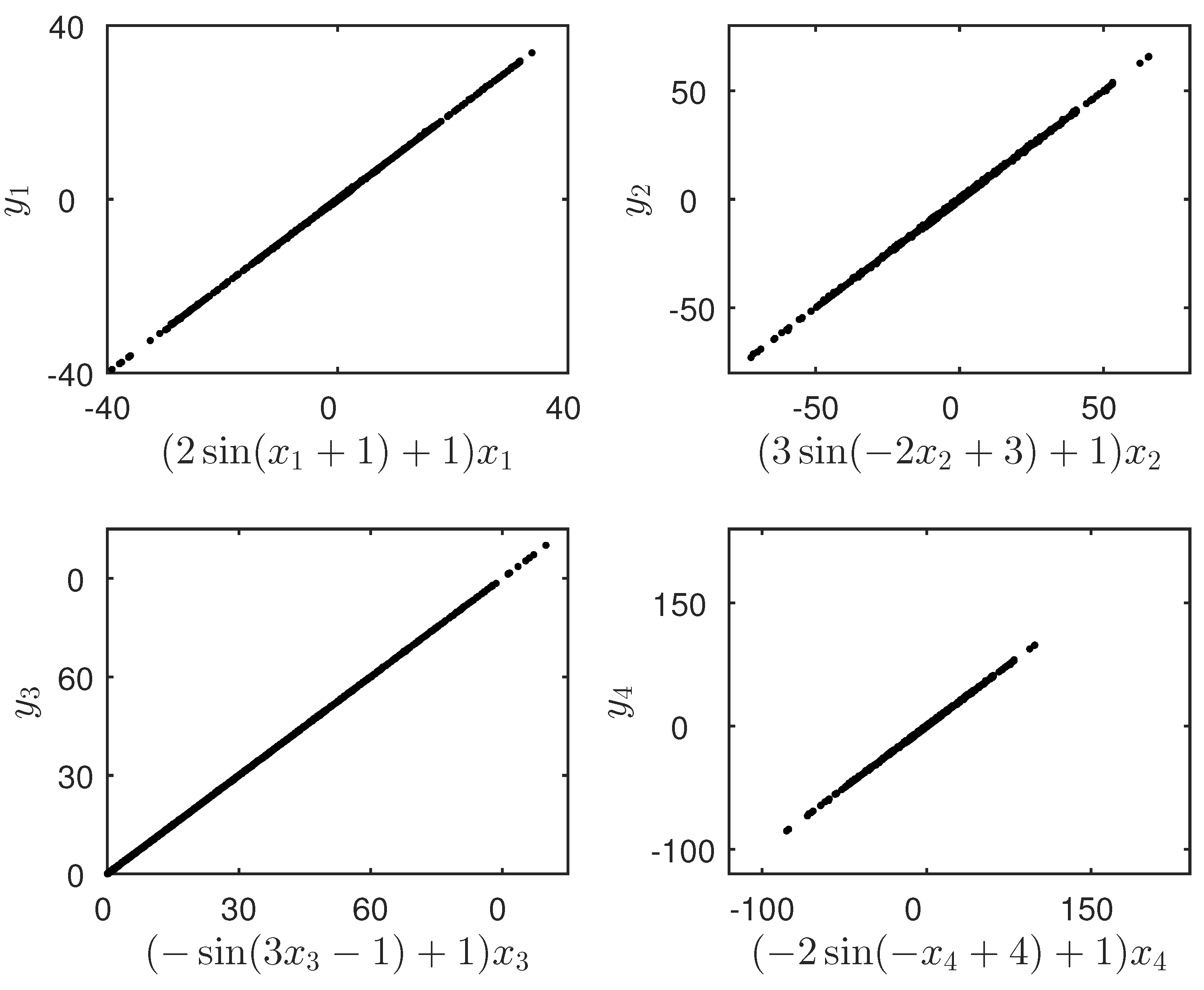The simulation results are shown in Figure 7 and Figure 8, which illustrate the validity of the parameter update laws (36) proposed in the section. It is worth pointing out that the parameter update laws (36) are still valid even if the scaling function factors are other complex functions.

6. Conclusions

In this paper, an adaptive controller is proposed to realize GFPS between two different chaotic systems (drive–response systems) with uncertain parameters based on the Laplace transform method. Compared to previous research, first, the uncertain chaotic systems considered in this paper are more generalized and have fewer restrictions on uncertain parameters; second, the GFPS scheme proposed in this paper is more generalized, and it can be used even when the scaling function factors are periodic functions, polynomial functions or other complex functions. Third, the parameter update laws designed for the estimation of uncertain parameters based on the GFPS condition derived using the Laplace transform method are simpler.

The greatest advantage of the GFPS scheme based on the Laplace transform method is that it can be used to design simple controllers and parameter update laws without constructing Lyapunov functions. The added controllers designed by this approach are more generalized and easier to realize physically than those designed through the Lyapunov function method.

It should be noted that we only consider the local stability of the origin in the GFPS error system between two chaotic systems in this paper. Moreover, to obtain the GFPS conditions, we require the smoothness of the trajectories in two chaotic systems to guarantee the existence, uniqueness and continuousness of solutions in a class of Volterra integral equations. According to the works in the literature [51,52], the global stability of the GFPS error system between two non-smooth chaotic systems is worthy of discussion, and this will be one of our next research points.

References

1. Pecora, L.M.; Carroll, T.L. Synchronization in chaotic systems. Phys. Rev. Lett. 1990, 64, 821–824. [Google Scholar] [CrossRef] [PubMed]
2. Carroll, T.L.; Pecora, L.M. Synchronizing chaotic circuits. IEEE Trans. Circ. Syst. I 1991, 38, 453–456. [Google Scholar] [CrossRef] [Green Version]
3. Chen, G.; Dong, X. From Chaos to Order: Methodologies, Perspectives and Applications; World Scientific: Singapore, 1998. [Google Scholar]
4. Klug, F. Synchronization transitions in supply chain networks. Int. J. Syst.-Sci.-Oper. Logist. 2023, 10, 2224104. [Google Scholar]
5. Zhong, X.H.; Jia, Z.W.; Li, Q.T.; Wang, L.S.; Guo, Y.Y.; Sun, Y.H.; Wang, Y.C.; Wang, A.B. Multi-wavelength broadband chaos generation and synchronization using long-cavity FP lasers. IEEE J. Sel. Top. Quantum Electron. 2023, 29, 0600207. [Google Scholar] [CrossRef]
6. Khezeli, M.; Najafi, E.; Molana, M.H.; Seidi, M. A sustainable and resilient supply chain (RS-SCM) by using synchronisation and load-sharing approach: Application in the oil and gas refinery. Int. J. Syst.-Sci.-Oper. Logist. 2023, 10, 2198055. [Google Scholar] [CrossRef]
7. Li, J.; Li, H.L.; Yang, J.P.; Yang, J.K.; Zhang, L. Hybrid control-based synchronization of fractional-order delayed complex-valued fuzzy neural networks. Comput. Appl. Math. 2023, 42, 154. [Google Scholar] [CrossRef]
8. Rosenblum, M.G.; Pikovsky, A.S.; Kurths, J. Phase synchronization of chaotic oscillators. Phys. Rev. Lett. 1996, 76, 1804–1807. [Google Scholar] [CrossRef] [Green Version]
9. Haerter, P.; Viana, R.L. Synchronization of phase oscillators due to nonlocal coupling mediated by the slow diffusion of a substance. Braz. J. Phys. 2023, 53, 114. [Google Scholar] [CrossRef]
10. Cao, L.; Lai, Y. Antiphase synchronism in chaotic systems. Phys. Rev. E 1998, 58, 382–386. [Google Scholar] [CrossRef] [Green Version]
11. Thazhathethil, R.; Pallimanhiyil, A.S. In-phase and anti-phase bursting dynamics and synchronisation scenario in neural network by varying coupling phase. J. Biol. Phys. 2023. [Google Scholar] [CrossRef]
12. Rosenblum, M.G.; Pikovsky, A.S.; Kurths, J. From phase to lag synchronization in coupled chaotic oscillators. Phys. Rev. Lett. 1997, 78, 4193–4296. [Google Scholar] [CrossRef]
13. Kumar, V.; Heiland, J.; Benner, P. Exponential lag synchronization of Cohen-Grossberg neural networks with discrete and distributed delays on time scales. Neural Process. Lett. 2023. [Google Scholar] [CrossRef]
14. Kocarev, L.; Parlitz, U. Generalized synchronization, predictability, and equivalence of unidirectionally coupled dynamical systems. Phys. Rev. Lett. 1996, 76, 181–1819. [Google Scholar] [CrossRef] [PubMed] [Green Version]
15. Xing, Y.A.; Dong, W.J.; Zeng, J.; Guo, P.T.; Zhang, J.; Ding, Q. Study of generalized chaotic synchronization method incorporating error-feedback coefficients. Entropy 2023, 25, 818. [Google Scholar] [CrossRef]
16. Mainieri, R.; Rehacek, J. Projective synchronization in the threedimensional chaotic systems. Phys. Rev. Lett. 1999, 82, 3042–3045. [Google Scholar] [CrossRef]
17. Han, J.; Chen, G.C.; Wang, L.M.; Zhang, G.D.; Hu, J.H. Direct approach on fixed-time stabilization and projective synchronization of inertial neural networks with mixed delays. Neurocomputing 2023, 535, 97–106. [Google Scholar] [CrossRef]
18. Chee, C.Y.; Xu, D.L. Chaos-based M-nary digital communication technique using controlled projective synchronization. IEEE Proc. Circuits Devices Syst. 2006, 153, 357–360. [Google Scholar] [CrossRef]
19. Zhang, F.F.; Leng, S.; Li, Z.F.; Jiang, C.M. Time delay complex Chen chaotic system and secure communication scheme for wireless body area networks. Entropy 2020, 22, 1420. [Google Scholar] [CrossRef]
20. Baluni, S.; Yadav, V.K.; Das, S. Quasi projective synchronization of time varying delayed complex valued Cohen-Grossberg neural networks. Inf. Sci. 2022, 612, 231–240. [Google Scholar] [CrossRef]
21. Xu, D.L. Control of projective synchronization in chaotic systems. Phys. Rev. E. 2001, 63, 027201. [Google Scholar] [CrossRef]
22. Xin, B.G.; Wu, Z.H. Projective synchronization of chaotic discrete dynamical systems via linear state error feedback control. Entropy 2015, 17, 2677–2687. [Google Scholar] [CrossRef] [Green Version]
23. Wen, G.; Xu, D. Nonlinear observer control for full-state projective synchronization in chaotic continuous-time system. Chaos Solitons Fractals 2005, 26, 71–77. [Google Scholar] [CrossRef]
24. Yan, J.; Li, C. Generalized projective synchronization of a unified chaotic system. Chaos Solitons Fractals 2005, 26, 1119–1124. [Google Scholar] [CrossRef]
25. Zhou, Y.; Wang, H.; Liu, H. Generalized function projective synchronization of incommensurate fractional-order chaotic systems with inputs saturation. Int. J. Fuzzy Syst. 2019, 21, 823–836. [Google Scholar] [CrossRef]
26. Zhang, L.; Wang, Y.; Wang, Q.; Qiao, S.; Wang, F. Generalized projective synchronization for networks with one crucial node and different dimensional nodes via a single controller. Asian J. Control 2020, 24, 1471–1483. [Google Scholar] [CrossRef]
27. Li, X.; Zhao, X.; Lu, Y.; Xu, T.; Hou, P.; Cui, X. Generalized projection synchronization and generalized dislocation synchronization of fractional-order financial chaotic systems with different orders. In Proceedings of the International Symposium on Electrical, Electronics and Information Engineering, Soul, Republic of Korea, 19–21 February 2021; pp. 635–638. [Google Scholar]
28. Li, G.H. Modified projective synchronization of chaotic system. Chaos Solitons Fractals 2007, 32, 1786–1790. [Google Scholar] [CrossRef]
29. He, J.M.; Lei, T.F.; Chen, F.Q. Global matrix projective synchronization of delayed fractional-order neural networks. Soft Comput. 2023, 27, 8991–9000. [Google Scholar] [CrossRef]
30. Feng, C.F.; Tan, Y.R.; Wang, Y.H.; Yang, H.J. Active backstepping control of combined projective synchronization among different nonlinear systems. Automatika 2017, 58, 295–301. [Google Scholar] [CrossRef]
31. Chen, Y.; Li, X. Function projective synchronization between two identical chaotic systems. Int. J. Mod. Phys. C 2007, 18, 883–888. [Google Scholar] [CrossRef]
32. Chen, Y.; An, H.L. The function cascade synchronization approach with uncertain parameters or not for hyperchaotic systems. Appl. Math. Comput. 2008, 197, 96–110. [Google Scholar] [CrossRef] [Green Version]
33. El-Dessoky, M.M.; Alzahrani, E.O.; Almohammadi, N.A. Chaos control and function projective synchronization of noval chaotic dynamical system. J. Comput. Anal. Appl. 2019, 26, 1. [Google Scholar]
34. Bekiros, S.; Yao, Q.J.; Mou, J.; Alkhateeb, A.F.; Jahanshahi, H. Adaptive fixed-time robust control for function projective 332 synchronization of hyperchaotic economic systems with external perturbations. Chaos Solitons Fractals 2023, 172, 113609. [Google Scholar] [CrossRef]
35. Du, H.Y.; Zeng, Q.S.; Wang, C.H. Modified function projective synchronization of chaotic system. Chaos Solitons Fractals 2009, 197, 2399–2404. [Google Scholar] [CrossRef]
36. Srisuntorn, R.; Weera, W.; Botmart, T. Modified function projective synchronization of master-slave neural networks with mixed interval time-varying delays via intermittent feedback control. AIMS Math. 2022, 7, 18632–18661. [Google Scholar] [CrossRef]
37. Yu, Y.; Li, H.X. Adaptive generalized function projective synchronization of uncertain chaotic systems. Nonlinear Anal. RWA 2010, 11, 2456–2464. [Google Scholar] [CrossRef]
38. Li, Z.B.; Zhao, X.S. Generalized function projective synchronization of two different hyperchaotic systems with unknown parameters. Nonlinear Anal. RWA 2011, 12, 2607–2615. [Google Scholar] [CrossRef]
39. Wu, X.J.; Fu, Z.Y.; Kurths, J. A secure communication scheme based generalized function projective synchronization of a new 5D hyperchaotic system. Phys. Scr. 2015, 90, 045210. [Google Scholar] [CrossRef] [Green Version]
40. Al-Azzawi, S.F.; Al-Talib, Z.S. Generalized function projective synchronization via nonlinear controller strategy. J. Interdiscip. Math. 2022, 25, 1753–1765. [Google Scholar] [CrossRef]
41. Zhou, X.B.; Xiong, L.L.; Cai, X.M. Adaptive Switched Generalized Function Projective Synchronization between Two Hyperchaotic Systems with Unknown Parameters. Entropy 2013, 16, 377–388. [Google Scholar] [CrossRef]
42. Sun, J.W.; Guo, J.C.; Zhang, X.C. Adaptive generalized hybrid function projective dislocated synchronization of new four- dimensional uncertain chaotic systems. Appl. Math. Comput. 2015, 252, 304–314. [Google Scholar] [CrossRef]
43. Hamel, S.; Boulkroune, A. A generalized function projective synchronization sheme for uncertain chaotic systems subject to input nonlinearities. Int. J. Gen. Syst. 2016, 45, 689–710. [Google Scholar] [CrossRef]
44. Li, Z.B.; Tang, J.S. Generalized binary function projective synchronization of chaotic systems with unknown parameters. Optik 2017, 137, 101–107. [Google Scholar] [CrossRef]
45. Li, Q.P.; Liu, S.Y.; Chen, Y.G. Finite-time adaptive modified function projective multi-lag generalized compound synchronization for multiple uncertain chaotic systems. Int. J. Appl. Math. Comput. Sci. 2018, 28, 613–624. [Google Scholar] [CrossRef] [Green Version]
46. Abarbanel, H.D.I.; Rulkov, N.F.; Sushchik, M.M. Gneralized synchronization of chaos: The auxiliary system approach. Phys. Rev. E 1996, 53, 4528–4535. [Google Scholar] [CrossRef] [Green Version]
47. Nohel, J.A. Some problems in nonlinear Volterra integral equations. Bull. Am. Math. Soc. 1962, 68, 323–330. [Google Scholar] [CrossRef] [Green Version]
48. Kyrchei, I. Cramer’s rule for generalized inverse solutions. In Advances in Linear Algebra Research; Kyrchei, I., Ed.; Nova Science Publishers: Hauppauge, NY, USA, 2015; pp. 79–132. [Google Scholar]
49. Lorenz, E.N. Deterministic nonperiodic flow. J. Atmos. Sci. 1963, 20, 130–141. [Google Scholar] [CrossRef]
50. Chen, G.; Ueta, T. Yet another chaotic attrator. Int. J. Bifurc. Chaos 1999, 9, 1465–1466. [Google Scholar] [CrossRef]
51. Zhang, T.W.; Xiong, L.L. Periodic motion for impulsive fractional functional differential equations with piecewise Caputo derivative. Appl. Math. Lett. 2020, 101, 106072. [Google Scholar] [CrossRef]
52. Liu, Y.T. Global exponential stability and synchronization of discrete-time fuzzy bidirectional associative memory neural networks via Mittag-Leffler difference approach. Int. J. Fuzzy Syst. 2023, 25, 1922–1934. [Google Scholar] [CrossRef]
Figure 1. GFPS between systems (26) and (27) is achieved with the scaling function matrix h ( x ) = d i a g { 2 s i n ( x 1 + 1 ) + 1 , 3 s i n ( 2 x 2 + 3 ) + 1 , s i n ( 3 x 3 1 ) + 1 , 2 s i n ( x 4 + 4 ) + 1 } and K matrix (34).
Applsci 13 08135 g001
Figure 2. The estimates of the uncertain parameters of systems (26) and (27) for GFPS with the scaling function matrix h ( x ) = d i a g { 2 s i n ( x 1 + 1 ) + 1 , 3 s i n ( 2 x 2 + 3 ) + 1 , s i n ( 3 x 3 1 ) + 1 , 2 s i n ( x 4 + 4 ) + 1 } and K matrix (34). (a) uncertain parameters in system (26) (b) uncertain parameters in system (27).
Applsci 13 08135 g002
Figure 3. GFPS between systems (26) and (27) is achieved with the scaling function matrix h ( x ) = d i a g { 2 s i n ( x 1 + 1 ) + 1 , 3 s i n ( 2 x 2 + 3 ) + 1 , s i n ( 3 x 3 1 ) + 1 , 2 s i n ( x 4 + 4 ) + 1 } and K matrix (35).
Applsci 13 08135 g003
Figure 4. The estimates of the uncertain parameters of systems (26) and (27) for GFPS with the scaling function matrix h ( x ) = d i a g { 2 s i n ( x 1 + 1 ) + 1 , 3 s i n ( 2 x 2 + 3 ) + 1 , s i n ( 3 x 3 1 ) + 1 , 2 s i n ( x 4 + 4 ) + 1 } and K matrix (35). (a) uncertain parameters in system (26) (b) uncertain parameters in system (27).
Applsci 13 08135 g004
Figure 5. GFPS between systems (38) and (39) is achieved with the scaling function matrix h ( x ) = d i a g { 2 s i n ( x 1 + 1 ) + 1 , 3 s i n ( 2 x 2 + 3 ) + 1 , s i n ( 3 x 3 1 ) + 1 ) } . (a) ( 2 s i n ( x 1 + 1 ) + 1 ) x 1 vs. y 1 (b) ( 3 s i n ( 2 x 2 + 3 ) + 1 ) x 2 vs. y 2 (c) ( s i n ( 3 x 3 1 ) + 1 ) ) x 3 vs. y 3 .
Applsci 13 08135 g005
Figure 6. The estimates of the uncertain parameters of systems (38) and (39) for GFPS with the scaling function matrix h ( x ) = d i a g { 2 s i n ( x 1 + 1 ) + 1 , 3 s i n ( 2 x 2 + 3 ) + 1 , s i n ( 3 x 3 1 ) + 1 ) } . (a) uncertain parameters in system (38) (b) uncertain parameters in system (39).
Applsci 13 08135 g006
Figure 7. GFPS between systems (38) and (39) is achieved with the scaling function matrix h ( x ) = d i a g { 0.02 x 1 2 + 0.2 x 1 + 1 , 0.01 x 2 2 + 0.1 x 2 1 , 0.03 x 3 2 0.1 x 3 + 0.5 ) } . (a) ( 0.02 x 1 2 + 0.2 x 1 + 1 ) x 1 vs. y 1 (b) ( 0.01 x 2 2 + 0.1 x 2 1 ) x 2 vs. y 2 (c) ( 0.03 x 3 2 0.1 x 3 + 0.5 ) x 3 vs. y 3 .
Applsci 13 08135 g007
Figure 8. The estimates of the uncertain parameters of systems (38) and (39) for GFPS with the scaling function matrix h ( x ) = d i a g { 0.02 x 1 2 + 0.2 x 1 + 1 , 0.01 x 2 2 + 0.1 x 2 1 , 0.03 x 3 2 0.1 x 3 + 0.5 } . (a) uncertain parameters in system (38) (b) uncertain parameters in system (39).
Applsci 13 08135 g008
Disclaimer/Publisher’s Note: The statements, opinions and data contained in all publications are solely those of the individual author(s) and contributor(s) and not of MDPI and/or the editor(s). MDPI and/or the editor(s) disclaim responsibility for any injury to people or property resulting from any ideas, methods, instructions or products referred to in the content.