A Multi-Scale Deep Back-Projection Backbone for Face Super-Resolution with Diffusion Models

Abstract

Face verification and recognition are important tasks that have made great progress in recent years. However, recognizing low-resolution faces from small images is still a difficult problem. In this paper, we advocate using diffusion models (DMs) to enhance face resolution and improve their quality for various downstream applications. Most existing DMs for super-resolution use U-Net as their backbone network, which only exploits multi-scale features along the spatial dimension. These approaches result in a slow convergence of corresponding DMs and the inability to capture complex details and fine textures. To address this issue, we propose a novel conditional generative model based on DMs called BPSR3, which replaces the U-Net in super-resolution via repeated refinement (SR3) with a multi-scale deep back-projection network structure. BPSR3 can extract richer features not only in depth but also in breadth. This helps to effectively refine the image quality at different scales. The experimental results on facial datasets show that BPSR3 significantly improved both convergence speed and reconstruction performance. BPSR3 has about 1/4 of the parameters of SR3 but achieves a 50.1% improvement in PSNR, a 19.8% improvement in SSIM, and a 15.4% reduction in FID. Our contribution lies in achieving less time and space consumption and better reconstruction results. In addition, we propose an idea of enhancing the performance of DMs by replacing the U-Net with a better network.

1. Introduction

Face verification and recognition have advanced significantly in recent years, but recognizing LR faces from small-sized images is still challenging. These facial images often lack visual clues and are difficult to differentiate from other small objects. This results in a low accuracy for LR face detection. Super-resolution (SR) reconstruction of facial images can alleviate this problem. Single image super-resolution (SISR) is a computer vision task that aims to restore high-resolution (HR) images from low-resolution (LR) images. This is challenging because the image degradation process is not standardized and different HR images can degrade to the same LR image.

SR reconstruction based on convolutional neural networks (CNN) often outperforms traditional methods due to its powerful ability to capture complex mappings. Despite their imperfections [1], CNN-based models have demonstrated an outstanding performance across a variety of computer vision applications [2,3]. SRCNN [4] is the first CNN-based SISR model and it outperforms many traditional models. Following its success, many scholars have also applied CNN to SISR, such as Very Deep Convolutional Networks [5] and Deeply Recursive Convolutional Networks [6]. Among these approaches, Haris M et al. [7] proposed a deep back-projection network (DBPN), which inspired our later work. In terms of face reconstruction, CNN has also achieved some success. Yun et al. [8] proposed an adversarial framework combined with CNN to reconstruct the HR facial image by simultaneously generating an HR image with and without blur. Grm et al. [9] proposed a cascade of multiple CNN-based SR models that progressively upscale the LR images by factors of 2×. They addressed the problem of hallucinating HR facial images from unaligned LR inputs at high magnification factors.

Since the introduction of the generative adversarial networks (GANs) [10], SISR based on GANs has gained popularity, as seen in [11,12,13,14,15,16,17]. Recently, however, diffusion models [18] with rigorous mathematical inference have surpassed the previous SOTA GAN in some tasks, such as image generation [19], and image synthesis [20,21]. Diffusion models are a type of image generation models that simulates the image degradation process by gradually adding noise and learning the distribution of the real image through the denoising process. By adding a small amount of noise at each step, these models achieve better results. Nevertheless, several challenges persist. For instance, the training process of diffusion models is computationally demanding due to the multiple repeated sampling. Moreover, convergence can be slow, and there are instances where the reconstructed output fails to align adequately with the reference image.

Several researchers are currently addressing these concerns and solving the drawbacks of the diffusion models mentioned above. Li et al. [22] proposed an efficient diffusion-based SISR approach that reduces training costs by diffusing the residual between HR and LR images. Saharia C et al. [23] introduced a generalized conditional generative SISR method that directly generates HR images by using LR image-guided diffusion. However, this method requires stitching LR images and involves a significant computational effort. Shang et al. [24] utilized residual diffusion for SISR, incorporating a CNN in image preprocessing to capture improved pixel neighborhood relations. To tackle a slow convergence, Hoogeboom E et al. [25] and Bao et al. [26] replaced the U-Net architecture underlying the diffusion model with transformer-based modules. Meanwhile, they introduced an accelerated sampling scheme and achieved promising results. In addition, researchers have proposed accelerated sampling methods [27,28] to address non-Gaussian and multimodal distributions in the inverse diffusion process.

This paper aims to enhance the application of diffusion models in facial image SR by leveraging their strengths in combination. Inspired by the findings from Haris M et al. [7], Saharia C et al. [23], Shang et al. [24], and Hoogeboom E et al. [25], we propose BPSR3, a conditional generation diffusion model that replaces the U-Net with a multi-scale DBPN, and apply it to the SISR task. BPSR3 follows the idea of SR3 [23] using LR directly to guide the reconstruction of images and keeping the same parameter continuity settings as SR3. Meanwhile, we note that Simple Diffusion [25] demonstrated the usability of replacing the underlying network, ResDiff [24] found the effectiveness of using a convolutional structure to guide the reconstruction, and DBPN [7] achieved some success in SISR. Therefore, we tried to replace the U-Net with a structure from the DBPN family, through which the scaling is conducted in the convolutional structure. Unlike in Simple Diffusion, we completely discarded the U-shaped structure in our proposed model and instead completed the network replacement by splicing parallel sequences formed by DBPNs with different scales. The different scales allow the DBPN to capture information at multiple image scales like U-Net. The skip connections in the DBPN help the diffusion model enhancement to preserve the Markov condition, making the results at a certain time step depend on previous or subsequent effects. Such a parallel structure approach boasts a reduced parameter count compared to the traditional U-Net, thereby simplifying the model and aiding in the reduction in training costs while accelerating convergence. Furthermore, at the zoom level of the image, leveraging convolution operations enables a more precise extraction of pixel proximity compared to interpolation methods. This enhancement leads to improved reproduction of the reconstruction.

Our experiments on facial datasets show that (1) BPSR3 has only 1/4 of the parameters of SR3 and converges faster and more stably; (2) BPSR3’s multi-scale design is more effective than single-scale; and (3) BPSR3 can reconstruct HR images without affecting the potential for accelerated sampling.

Our contribution to face SR can be summarized as follows:

Less time and space consumption: we propose a multi-scale BP-based diffusion model BPSR3 for the facial SISR task, which improves the reconstruction convergence speed significantly compared to SR3 using U-Net. Moreover, BPSR3 uses fewer parameters and computes fewer feature maps for the same magnification task. It achieves successful optimization in both time and space.

More restored reconstruction results: using learnable convolutional structures to scale images can capture the image domain relationships better than U-Net with linear interpolation methods. This can enhance the visual similarity between their constructed image and the reference image.

2. Related Work

2.1. Single-Scale Deep Back-Projection Networks

SISR is a challenging task that aims to reconstruct an HR image from an LR image. This task has many applications in various fields, such as satellite imagery [29], monitoring equipment [30], remote sensing images [31], medical imaging [32], and so on. However, SISR is an ill-posed problem because one LR image can correspond to multiple HR images. Therefore, it requires sophisticated methods to recover the missing details and enhance the image quality.

Deep learning methods have become popular for SISR in recent years. Haris M et al. [7] proposed DBPN, which uses iterative up and down sampling layers to provide an error feedback mechanism for projection errors at each stage. It improves SR performance for large scaling factors by bringing high-level information back to the previous layer and refining low-level information. Based on DBPN [7], Geng et al. [33] proposed an enhanced back-projection network that provides an up and down sampling process with error feedback to capture various spatial correlations and introduced the residual block in the sampling process to alleviate the difficulty of training deep networks.

By constructing interconnected upward and downward sampling stages, the DBPN can handle different types of image degradation and recover HR components. To conclude, the DBPN offers three valuable insights for SISR: (1) jump connection; (2) continuous up and down sampling; and (3) sampling with convolution.

2.2. SISR Based on the Conditional Diffusion Model

Diffusion models are a type of image generation models that is inspired by nonequilibrium thermodynamics. It defines a Markov chain of diffusion steps (the current state is only related to the previous state) and learns the reverse diffusion process to reconstruct the original data from noise. This model can be used for tasks such as image smoothing, denoising, and image generation. In image generation, the diffusion model can iteratively update pixels to produce diverse and realistic images. In terms of SISR, diffusion models can increase the detail and quality of an image by denoising it from additive Gaussian noise.

Li et al. [22] proposed a novel approach to SISR by leveraging diffusion models, which efficiently diffuse the residual between HR and LR images to reduce training costs. By combining joint diffusion results with the LR image’s residual, their approach achieves SOTA performance in generating HR images at that period. Saharia C et al. [23] proposed a more generalized generative SISR method that generates HR images directly using LR image-guided diffusion derived from other conditional generation scenarios. However, this approach requires stitching LR images and incurs a huge computational effort. The diffusion models need to recover both the high- and low-frequency content of the image, which prolongs the convergence time and may inhibit the model’s attention to fine-grained information and texture details, leading to generating images that deviate further from the reference image. Similarly, Shang et al. [24] used residual diffusion for SISR but incorporated a CNN in image preprocessing to capture better pixel neighborhood relations, as opposed to [22], which used interpolation.

2.3. Replacement of U-Net in Diffusion Models

Almost all diffusion models recently use U-Net as the base network. Therefore, a very natural question arises: whether the reliance on the U-Net is necessary for diffusion models.

Some academics have successfully replaced it with a transformer-based architecture: Bao et al. [26] designed a simple and general ViT-based architecture called U-ViT. Following the design methodology of transformers, U-ViT treats all inputs including the time, condition, and noisy image patches as tokens. Hoogeboom E et al. [25] used a series of similar transformer modules to replace the U-Net in the diffusion model, simplifying the diffusion model base network and providing a viable solution for single-training speedups. The successful experiments of these researchers demonstrate the possibility of using alternative models to U-Net, which inspires our research direction.

3. Image Super-Resolution via Repeated Refinement

3.1. Gaussian Diffusion Process

We were given a dataset of input–output image pairs, denoted $D={\{{LR}_i,{HR}_i\}}_{i=1}^N$, which represents samples drawn from an unknown distribution $p\left(HR|LR\right)$. The conditional distribution $p\left(HR|LR\right)$ is a one-to-many mapping in which many target HR images may be consistent with a single source LR image. In diffusion models, there are two crucial processes: the diffusion process and the inference process, both of which are parameterized Markov chains. We refer to them as process $q$ and process $p$, respectively.

SR3 [23] learns the parameter estimation of $p\left(HR|LR\right)$ by a stochastic iterative refinement process based on DDPM [18], which maps the source image LR to the target image HR. The forward Markov process $q$ can be defined as follows:

$$q\left({HR}_{1:T}|{HR}_0\right)={\prod }_{t=1}^{T}q\left({HR}_t|{HR}_{t-1}\right),$$

(1)

$$q\left({HR}_t|{HR}_{t-1}\right)=\mathcal{N}\left({HR}_t|\sqrt{{\alpha }_t}{HR}_{t-1},\left({1-\alpha }_t\right)\mathit{I}\right),$$

(2)

where $0<{\alpha }_t<1(t=1,2,\dots ,T)$ is a scalar parameter, which determines the variance of the noise added at each iteration. We used t to represent a certain moment in the diffusion process $q$, and T to represent the end moment. T also corresponds to the inference step. Note that ${HR}_{t-1}$ is attenuated by $\sqrt{{\alpha }_t}$ to ensure that the variance of the random variables remains bounded as $t\to \mathrm{\infty }$. The original HR image ${HR}_0$ gradually loses its distinguishable features as the step t becomes larger. Eventually, after T iterations, ${HR}_T$ is equivalent to an isotropic Gaussian noise.

In addition, an important conclusion of the diffusion process is that the ${HR}_t$ image at any moment can be derived from the source image ${HR}_0$, as shown in Equation (3):

$$q\left({HR}_t\right|{HR}_0)=\mathcal{N}\left({HR}_t|\sqrt{{\gamma }_t}{HR}_0,(1-{\gamma }_t)\mathit{I}\right),$$

(3)

where ${\gamma }_t={\prod }_{i=1}^t{\alpha }_i$ $(t=1,2,\dots ,T)$. Since the ${\alpha }_i(i=1,2,\dots ,t)$ in the cumulative multiplication is a decimal, we can easily infer that ${\gamma }_t$ decreases as t increases. To make the diffusion and inverse diffusion process more continuous, SR3 [23] samples the hyperparameter ${\gamma }_t$ from a uniform distribution $p\left(\gamma \right)={\sum }_{i=1}^T\frac{1}{T}U({\gamma }_{t-1},{\gamma }_t)$. In the training phase, we sampled random pairs of time steps t to obtain a pre-defined sequence of hyperparameters ${\gamma }_t$. This is where iterative optimization takes place. Using uniformly distributed hyperparameters ${\gamma }_t$ makes the diffusion and inverse pre-post relationship more noticeable than using discrete time sampling.

3.2. Inference Process and Optimization Model

The inference process $p$ is the inverse of the process $q$, which starts from a pure Gaussian noise and goes in the reverse direction of the forward diffusion process. Combining Equations (2) and (3), and Bayes’ rule [18], we can derive the posterior distribution of ${HR}_{t-1}$ $(t=1,2,\dots ,T)$ given (${HR}_0$, ${HR}_{\mathrm{t}}$) as Equation (4):

$$\begin{gathered} q\left(H{R}_{t-1}∣{HR}_0,{HR}_t\right)=\mathcal{N}\left(H{R}_{t-1}∣\mathit{\mu },{\sigma }^2\mathit{I}\right), \\ \mathit{\mu }=\frac{\sqrt{{\gamma }_{t-1}}\left(1-{\alpha }_t\right)}{1-{\gamma }_t}{HR}_0+\frac{\sqrt{{\alpha }_t}\left(1-{\gamma }_{t-1}\right)}{1-{\gamma }_t}{HR}_t, \\ {\sigma }^2=\frac{\left(1-{\gamma }_{t-1}\right)\left(1-{\alpha }_t\right)}{1-{\gamma }_t}. \end{gathered}$$

(4)

Equation (4) shows how the “${\alpha }_t$ determines the variance of the noise added at each iteration” by giving the mean and variance of the noise-added image $H{R}_{t-1}$. This formula tells us that the variance of the inference $p$ at any time t can be decided with a pre-set sequence of hyperparameters ${\gamma }_t$. For the process $p$, $H{R}_t$ is always known, but $H{R}_0$ is unknown, which leads to the unknown mean $\mathit{\mu }$ of $H{R}_{t-1}$. But fortunately, according to Equation (3) and properties of the Gaussian distribution, we can use $H{R}_t$ to represent $H{R}_0$:

$$\begin{array}{c}{HR}_0=\frac{1}{\sqrt{{\gamma }_t}}\left({HR}_t-\sqrt{1-{\gamma }_t}{\mathit{ϵ}}_t\right),\end{array}$$

(5)

where ${\mathit{ϵ}}_t~\mathcal{N}(0,\mathit{I})$. If we plug Equation (5) into the expression for $\mathit{\mu }$, we can obtain a new mean expression that only involves ${HR}_t$ and a normal random variable ${\mathit{ϵ}}_t$. Since ${\mathit{ϵ}}_t$ is the only unknown factor, we can model it by letting a network $f_{\theta }$ output a prediction for ${\mathit{ϵ}}_t$. Furtherly, we can calculate the $\mathit{\mu }$ based on ${\mathit{ϵ}}_t$, and then obtain the result of $H{R}_{t-1}$.

Through a series of mathematical derivations and some simplification methods [23], each iteration of iterative refinement takes the form,

$${HR}_{t-1}\leftarrow \frac{1}{\sqrt{{\alpha }_t}}({HR}_t-\frac{1-{\alpha }_t}{\sqrt{1-{\gamma }_t}}{f}_{\theta }(LR,{HR}_t,{\gamma }_t\left)\right)+\sqrt{1-{\alpha }_t}{\mathit{ϵ}}_t).$$

(6)

In Equation (6), $f_{\theta }$ represents a network structure for stepwise noise reduction in the process $p$. The parameters of $f_{\theta }$ are learned in the training phase throughout the conditional diffusion model, which in turn enables inference to produce better-quality images. $f_{\theta }$ first up-samples the LR image with interpolation, and then concatenates the up-sampled LR with ${HR}_t$ to obtain a richer feature. We will discuss the causes of generation and optimal settings for $f_{\theta }$ in Section 4. Further, the optimized target model in the training process can be determined by using $f_{\theta }$ as Equation (7):

$$\min {\mathbb{E}}_{(LR,HR)}{\mathbb{E}}_{ϵ,{\gamma }_t}{\parallel f_{\theta }(LR,\sqrt{{\gamma }_t}{HR}_0+\sqrt{1-{\gamma }_t}ϵ,{\gamma }_t)-ϵ\parallel }_p^p,$$

(7)

where $ϵ~\mathcal{N}(0,\mathit{I})$, $(LR,HR)$ are sampled from the training set, $p$ can take the value 1 or 2, and the distribution of ${\gamma }_t$ is consistent with the sequence given in Section 3.1. To explain the diffusion model more clearly, we give Figure 1, which shows the entire SR3 operational flow. As shown in Figure 1, all $Ne{t}^t(t=1,2,\dots ,T)$ constitute a complete $f_{\theta }$. These sub-networks are abstract representations, and we did not train them separately. Instead, we controlled the network weights at different time steps through the hyperparameter ${\gamma }_t$.

As illustrated in Figure 1, during the training phase, the process of reconstructing an LR image involves several steps. Initially, the LR image is interpolated to the target size for reconstruction, such as scaling up a 64 × 64 LR image by a factor of four to obtain a 512 × 512 image through interpolation. This interpolated and scaled image is referred to as “Ref” and serves as auxiliary information to guide image generation.

The reference HR image, denoted as ${HR}_0$, is combined with Ref to generate the initial six image features. These features are then fed into the first base network, $Ne{t}^1$, which produces the noise-added image ${HR}_1$. Ref is spliced with ${HR}_1$ and the resulting image is then fed into $Ne{t}^2$, generating the noise-added image ${HR}_2$. This process is repeated for T steps, resulting in a sequence of noise-added images ${HR}_1$, ${HR}_2$, and so on, until reaching ${HR}_T$, which represents a pure Gaussian noise image.

During the inference process, Ref is utilized to reconstruct ${HR}_0$ from the same pure Gaussian noise image by backtracking step by step. As this paper is concerned with the underlying network in the diffusion model, readers who wish to investigate the mathematical principles of the diffusion model further can refer to the original SR3 [23].

4. Base Networks

This section focuses on the selection of $f_{\theta }$, including both the classical and the replaced network.

4.1. U-Net Architecture

U-Net [34] is a deep learning image segmentation model proposed by Ronneberger et al. in 2015. It has a symmetric encoder and decoder structure that resembles the letter U, hence its name. The current diffusion model still uses U-Net, which has been applied for a long time. The diffusion model based on U-Net performs well in practice and has also achieved some success in SR reconstruction [22,23,24,25,26].

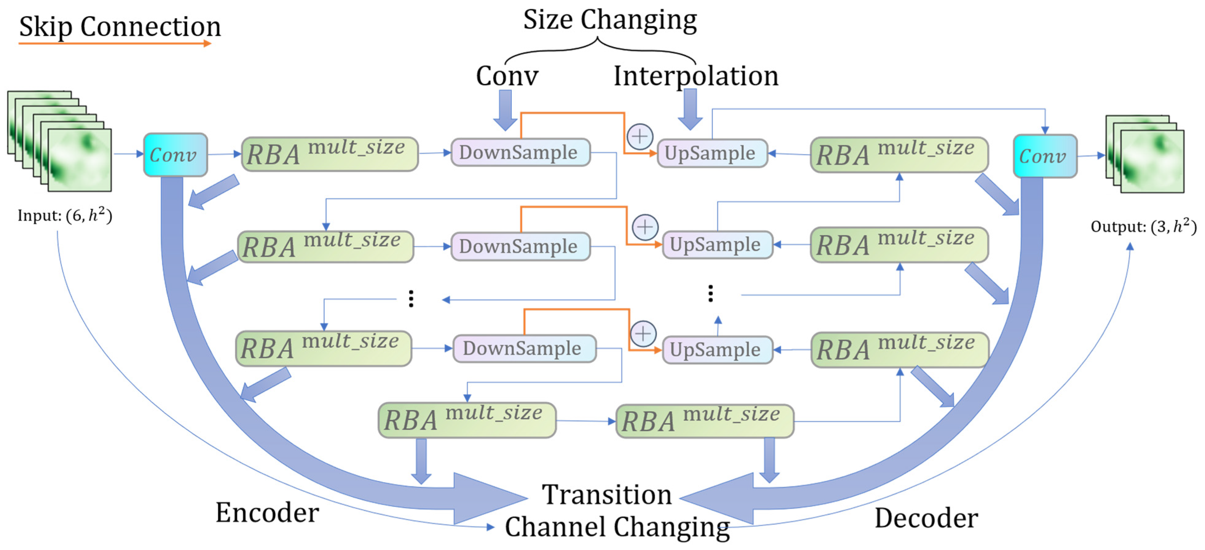
As shown in Figure 2, the original U-Net structure used in SR3 has three important types of modules: DownSample, UpSample, and ResnetBlockwitAttention (RBA).

The DownSample and UpSample modules do not change the number of extracted feature channels, and they are responsible for adjusting the image size to obtain information at multiple scales. The DownSample is implemented by using a convolution of size 3 × 3 with a step size of 2 and a circle around the zero-filled image. The UpSample is implemented by using an interpolation method. It is worth noting that during the up-sampling process, the input feature map will be spliced with the same size feature map obtained with the previous down-sampling, which is the so-called skip connection. The skip connections ensure that the features in the decoding process retain most of the original information while including high-frequency details and low-frequency contours.

RBA is composed of several residual blocks and an attention module that serves as a transition layer, which does not alter the size of the image but serves to enrich the feature representation; however, such a structure also induces temporal problems in the overhead.

Furthermore, we present a comprehensive exposition of the architecture of the U-Net depicted in Figure 2: the input is a concatenated LR and $H{R}_t$ image with six channels. After repeated up-sampling and down-sampling at different scales, a final RGB image with three channels was generated. Here, ${RBA}^{mult\_size}$ represents the RBA with a given feature growth sequence. In Figure 2, the channels of each RBA module increase exponentially from top to bottom based on the $mult\_size$ sequence and a basic channel number. For instance, if $mult\_size$ = {1, 2, 4, 8, 8}, and the basic channel number is 64, there are five groups of symmetric RBA modules that scale down the image to 1/32 of its original size. The first group outputs 64-channel features, the second group outputs 128-channel features, the third group outputs 256-channel features, and so on.

4.2. Deep Back-Projection Networks

DBPN utilizes iterative up- and down-sampling layers to achieve SISR reconstruction.

We noticed that DBPN has strong pre- and post-text connections: unlike the U-Net that concatenates feedback after some iterations, the alternating up and down structure of DBPN links the high-frequency and low-frequency information of the image during the iteration process, providing some error feedback mechanism.

We extend the idea of U-Net and used the DBPN modules to transfer information from the shallow to the deep part of the network. To avoid affecting the distribution of noise in the forward and backward process of the diffusion model, we reversed the order of ascending and descending in the original DBPN. This helps prevent the introduction of new noise due to image distortion at the beginning due to zooming in and out, and also reduces the overall image size, making fewer parameters to be trained and reducing the computational cost. The operation flow of the single DBPN module is depicted in Figure 3:

We denote the basic channel number, the scaling factor, the transition feature number, and the total number of stages as N_BC, s, F, and NS, respectively. The whole SR process consists of a feature extraction module, a Scale s module (including numerous multiple stages of down-sampling and up-sampling), and a reconstruction module.

First, the image passes through the feature extraction stage, where it uses convolution to extract F and N_BC features sequentially. Next, the feature will be subjected to continuous up-and-down sampling layers. These are layers that alternately up-sample and down-sample the feature by using convolution operations. This allows the model to learn from multiple scales and refine the output progressively. For example, if NS = 1, an h × h feature map is down-sampled to a size of (h/s) × (h/s) through convolution, and then up-sampled back to its original size through another convolution. This is repeated for multiple stages, with the number of output features remaining constant at N_BC, but the number of input features increases to N_BC × (1 + NS) at each stage. Finally, a transition convolution converts the output to three channels.

The s in the Scale s module determines the size of h/s shown in Figure 3. If s is 2, the size of the image will be transformed between h/2 and h. We can vary the length of the Scale s module to trade-off between feature richness and computational cost. In the BPSR3 proposed in Section 4.3.3 of this paper, we took three modules with s being 2, 4, and 8, respectively, and each module has six stages.

The DownBlock and UpBlock modules in DBPN, used for scaling, are mainly composed of convolutions. In Section 4.3, we provide a detailed description of these modules, combined with temporal encoding using the diffusion model.

We also tried to use the single DBPN directly as the base network of the diffusion model, but found an obvious failure phenomenon; this paper will not delve into this unsuccessful approach. In addition, in Section 5.3, we set up an ablation study to discuss the necessity of using multi-scale DBPN.

4.3. The BPSR3 Model

Building on the previous section, this section proposes the model BPSR3. The running part of the deep projection network given in Figure 3 can be resolved into three parts: a feature extraction module, a Scale s module, and a reconstruction module. Among them, the Scale s module is the core of DBPN. We extracted this module and used it as a basis to derive modules of DBPN for multiple scales. The feature extraction module extracts N_BC features, and the reconstruction module converts them to three channels for visualization. We treat these two modules as common components of multi-scale DBPN.

In the following, Section 4.3.1 explains the scaling sampling part and the corresponding temporal embedding considerations in detail, Section 4.3.2 gives an analogous story to illustrate our idea, and Section 4.3.3 details the model structure of BPSR3.

4.3.1. Scaling Sampling Module

The following is a detailed analysis of the

DownBlock and UpBlock submodules and the time code positions in the scaling sample, starting with the definition of some symbols:

$$\mathrm{scale}\mathrm{up}:H_0^t=(L^{t-1}\ast p_t){\uparrow }_s,$$

(8)

$$\mathrm{scale}\mathrm{down}:L_0^t=\left(H_0^t\ast g_t\right){\downarrow }_s,$$

(9)

$$\mathrm{residual}:e_t^l=L_0^t-L^{t-1},$$

(10)

$$\mathrm{scale}\mathrm{residual}\mathrm{up}:H_1^t=(e_t^l\ast q_t){\uparrow }_s,$$

(11)

$$\mathrm{output}\mathrm{feature}\mathrm{map}:H^t=H_0^t+H_1^t,$$

(12)

where * represents the spatial convolution operation, ${\uparrow }_s$ and ${\downarrow }_s$ represent the up-sampling and down-sampling operator at scaling scale $s$, respectively, and $p_t,g_t$, and $q_t$ are the (de)convolutional layers at stage $t$.

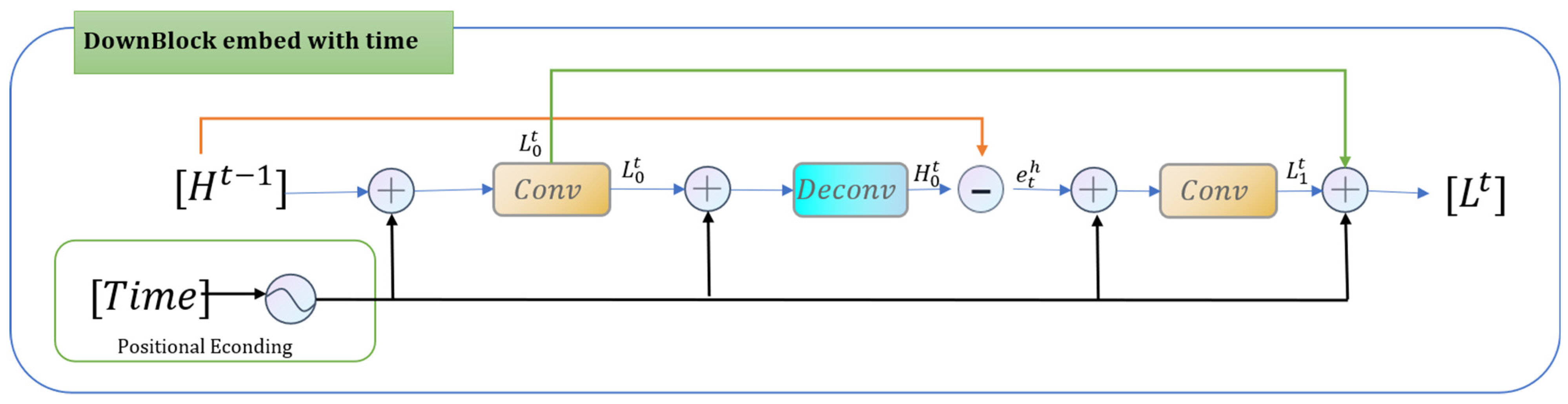
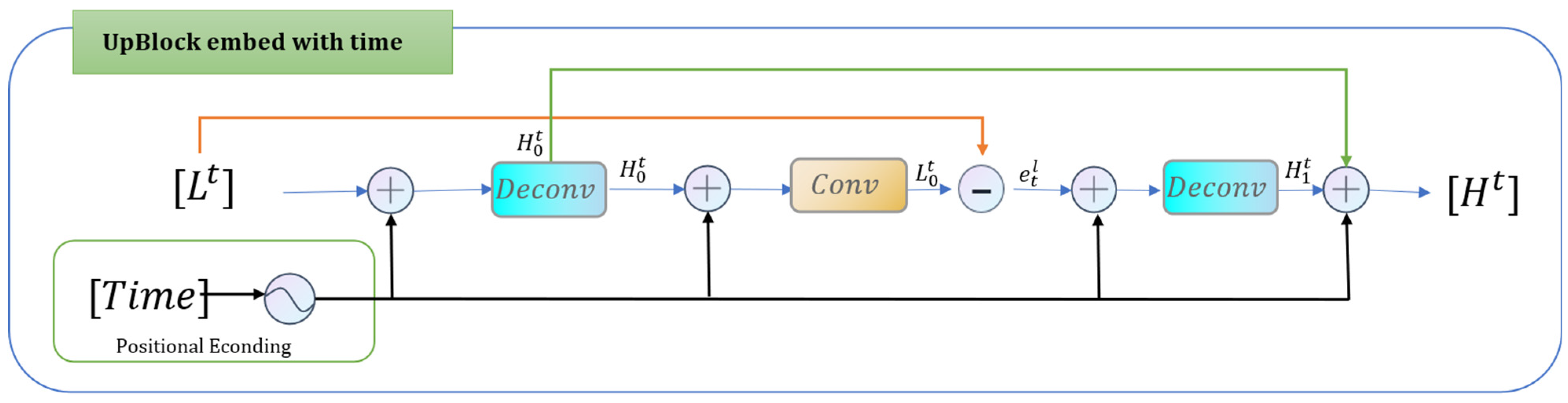
Equations (8)–(12) express the detailed process in the UpBlock in Figure 3. The previously calculated LR feature mapping $L^{t-1}$ was taken as input and mapped to the intermediate HR feature $H_0^t$, and then an attempt was made to map it back to LR space to obtain $L_0^t$ (this is the reverse projection), at which point the LR space residuals $e_t^l$ were generated, and the residuals were up-sampled to simulate the residuals in HR space and output together with $H_0^t$. We embedded the time into all the features before and after the convolution operation occurred, and its running flow is shown in Figure 4. Similarly, by reversing the input LR and output HR, we can obtain the time-embedded DownBlock module, which runs as shown in Figure 5.

4.3.2. Substitution Thinking

Our study drew inspiration from a pass-along guessing game. Imagine there are three teams consisting of graduate students, middle school students, and elementary school students, each with two members. These teams are arranged in a symmetrical order based on their level of education, from highest to lowest and then back to highest. The game involves passing a puzzle from one person to another, starting with a graduate student and going through each person’s description of the puzzle until it reaches the graduate student on the other side.

In this game, people with the same education level can communicate with each other, which is similar to the concept of the jump connection in U-Net. However, the information described by individuals with different education levels varies. This is because the depth of academic knowledge influences how well people can describe and understand things accurately. For instance, if the puzzle is about the biological classification of starfish, a graduate student may know the answer and pass it backward, but a middle school student might only understand the keyword “starfish” and pass that along, while an elementary school student may provide a general description of a star shape. Even if the final graduate student has the right knowledge, the correct answer may not be reached due to information loss during the transmission process.

In U-Net, a similar series of convolution operations represents the transfer of information, which involves a loss of information along the way.

Skip connections (as indicated by the orange line in Figure 2) allow the tail end to access the information from the head end, which can preserve some information. However, the effectiveness of skip connections depends on the knowledge level of the students at both ends. If one of them is clueless about ‘starfish’, then skip connections are useless. In this case, normal information transmission (without the skip connection) may be helpful. On the other hand, if both students are familiar with the answer, then normal information transmission may be disruptive and harmful.

Based on this analogy, we infer that U-Net suffers from information loss during propagation and that skip connections can mitigate this issue by providing multi-scale information. These insights guide our choice of the next network.

4.3.3. Serial and Parallel Architecture

Previously, we mentioned three important modules of DBPN: a feature extraction module, a Scale s module, and a reconstruction module. To avoid redundancy of feature extraction and reduce computation, we designed multi-scale DBPN with a common feature extraction module and reconstruction module for each scale. We combined Scale s modules with different s, as shown in Figure 6.

Figure 6 is a parallel structure where the initialized features are applied simultaneously to the Scale s module at different scales, and finally stitched together to form the features and output the results.

In the parallel structure, modules of scale s at each scale operate independently, unaffected by modules at other scales. This design minimizes the potential loss of information that could occur due to deep feedforward propagation. At the same time, DBPN at one scale has a multi-stage continuous jump connection, which makes the information propagation process without too much deviation.

Our BPSR3 allows for the extraction of image features at different scales, facilitated by its breadth. The individual DBPN submodules, which are elongated freely, ensure that we can learn features with different depths. By combining the parallel structure from Figure 6 with the insights provided in Section 4.3.1, we present a comprehensive explanation of the network operation structure in BPSR3.

Suppose that we are in the step of t in either diffusion or inference. When the LR image is combined with the HR image corresponding to the current step, a six-channel feature representation is formed. The Initial Feature Extraction module performs convolution on this representation to extract a new base filter of features. These features then traverse through the different scale modules.

Taking Scale 2 as an example, as shown in Figure 3, the shallow feature map enters the sequence and is initially down-sampled by a factor of 2. Subsequently, it is restored to its original size through up-sampling. This process is repeated for several rounds, where the previous features are added to the subsequent ones. Consequently, the number of input channels increases linearly, while the number of output channels remains the same. The remaining DBPN sequences follow a similar process as Scale 2.

The DBPN at each scale will obtain N_BC features. Assuming that there are such NB Scale s modules, the features obtained by these sequences are spliced to obtain N_BC × NB features. In our follow-up experiments, we set NB = 3.

Finally, after a transitional convolutional layer (the reconstruction module), the number of feature channels comes to three. Specially, in the whole process, positional encoding [35] is conducted in the feature extraction module, each Scale s module, and the reconstruction module.

5. Experiment

To evaluate the performance of BPSR3 on face reconstruction, we set up a comparison experiment with SR3 and some ablation experiments to verify the effectiveness of its structure. The evaluation metrics chosen include two distortion-based metrics, PSNR and SSIM [36], and one perception-based metric, FID [37]. For the sake of fairness, BPSR3 used the same dataset when compared with other algorithms. We give the code for BPSR3 in the Supplementary Material.

5.1. BPSR3 Basic Configuration

For all BPSR3 (4×) below, if not otherwise specified, the parameters were optimized using the Adam [38] optimizer. The initial learning rate of the optimizer was set to $1\times {10}^{-4}$, and other related parameters were taken as a default. We set the batch size to 4, T to 1000, and the hyperparameter value of ${\beta }_{1:T}$ (${\beta }_t$ is equivalent to 1 − ${\alpha }_t$ and $t=1,2,\dots ,T$) grew linearly from $1\times {10}^{-6}$ to $1\times {10}^{-2}$. Following training, we obtained LR images by down-sampling HR images and used the source image as a reference for reconstruction.

We kept the same hyperparameters with SR3, except for U-Net, so we did not use k-fold cross-validation. Moreover, we did not use data augmentation, like SR3. This simplified the experimental process and reduced the consumption of computational resources.

We used a Tesla V100S-PCIE-32GB GPU to train and test our algorithm model on Pytorch 1.7.1 with Python 3.8.5.

5.2. Comparison with Other Algorithms on Face Images

BPSR3 was compared to the original baseline SR3 [23] using the face datasets CelebA [39] and FFHQ [40] on the 64 × 64 → 256 × 256 (4×) task. For baseline SR3, we followed SR3 to set $mult\_size$ = {1, 2, 4, 8, 8} and N_BC = 64. We used two residual blocks and a dropout with a value of 0.2. Except for these special parameters above, in the non-basic network parameters part of the diffusion model, the settings of SR3 were exactly the same as those of BPSR3.

We used about 30k of CelebA facial images to SR3 and BPSR3. For evaluation, we selected the first 10 images of FFHQ and computed the average PSNR and SSIM of their reconstructions. We saved the evaluation metrics and checkpoints every 10k iterations until we reached 0.5 M iterations. Figure 7 shows the comparison curves of model convergence speed and reconstruction effect.

It is easy to observe from Figure 7 that the PSNR and SSIM of BPSR3 fluctuate widely in the first 200 k iterations but stabilize at a higher value after 200 k. SR3 has almost no large variation between 0.5 M in PSNR, while its optimal value is far from the general level of BPSR3; in the SSIM performance, although SR3 also shows an upward trend, it still does not reach the general level of BPSR3. This indicates that SR3 converges slower than BPSR3.

We computed the parameter counts for SR3 and BPSR3 to be approximately 97 M and 25 M, respectively. Remarkably, the latter constitutes nearly a quarter of the former, indicating that we achieved superior reconstructions using a simpler model.

Furthermore, we evaluated several advanced algorithms on the same validation dataset, including Latent-Diffusion [20], SwinIR [41], RealESRGAN [42], and BSRGAN [43]. Among them, Latent-Diffusion is based on the diffusion model, SwinIR is based on Vision Transformer, and RealESRGAN and BSRGAN are based on GAN.

For evaluation, we measured PSNR, SSIM, and FID. We determined the optimal values for the training process of BPSR3 and its base model SR3. For the other models, we used the default options as given by the authors in the GitHub code.

According to

Table 1. The average performance of BPSR3 versus other SR reconstruction algorithms validated on the first 10 images of FFHQ (64 × 64 → 256 × 256).

Based	Models	PSNR↑	SSIM↑	FID↓
Transformer	SwinIR [41]	26.29	0.7796	113.652
Transformer	SwinIR (Large) [41]	27.20	0.8093	97.976
GAN	RealESRGAN [42]	26.42	0.7856	152.281
GAN	BSRGAN [43]	26.99	0.7901	120.312
Diffusion model	SR3 (The basic one) [23]	20.24	0.7174	77.147
Diffusion model	Latent-Diffusion [20]	26.47	0.7829	110.297
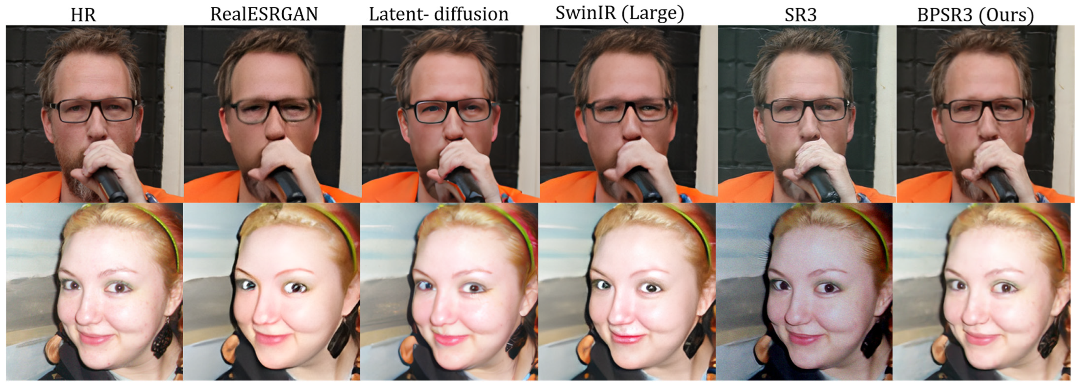
Diffusion model	BPSR3 (Ours)	30.37	0.8597	65.238

, it can be found that the BPSR3 proposed in this paper is optimal in all indicators, which shows its effectiveness. Further, we present Figure 8 to demonstrate the reconstruction results of some of the algorithms in Table 1 for a qualitative analysis. A more representative sample with more significant differences was selected for presentation.

Figure 8 demonstrates that, apart from the SR3 and BPSR3 algorithms, the reconstructed images tend to exhibit excessive smoothness. While SR3 maintains the overall shape of the original image, there is a noticeable variation in the primary hue. On the other hand, our BPSR3 reconstructions closely resemble the reference HR image, offering the most faithful restoration results.

5.3. Ablation Experiments on Face Images

To illustrate the necessity of multi-scale information, we compared DBPNs at different single scales on the same face dataset as in Section 5.2.

We trained different DBPN groups for 10 epochs and tested the 10th epoch on the first three images (a), (b), and (c) in FFHQ. Figure 9 shows the reconstruction results for each group.

For Figure 9, the HR column is the reference HR image; the Interpolation column is the reconstruction with linear interpolation only, while “Scale 8”, “Scale 4”, and “Scale 2” represent the reconstruction with DBPN scales of 8, 4, and 2, respectively; and “Scale 2–4–8” is the reconstruction with multiple scales in parallel. It is evident that the reconstruction of “Scale 8” is notably subpar, exhibiting considerable noise while displaying rough outlines.

The single-scale reconstructions of Scale 2 and Scale 4 are satisfactory, but they are blurry in detail compared to the multi-scale DBPN. For example, the eyes of Figure 9a,c, and the mouth of Figure 9b.

To quantitatively illustrate the effect of DBPN groups at several different scales, we calculated the FID, average PSNR, and average SSIM between HR and reconstructed images, as shown in

Table 2. Evaluation metrics for training 10 epochs when using DBPN at different scales as the base network (results are the average of tests on Figure 9a–c above).

DBPN Scale	FID↓	PSNR↑	SSIM↑
Scale 2	142.608	29.95	0.816
Scale 4	129.36	30.73	0.833
Scale 8	577.557	8.27	0.015
Scale 2–4–8	88.413	30.68	0.843

.

We observe that the multi-scale DBPN, despite having a slightly lower PSNR, achieves the best performance in both SSIM and FID for the same number of training iterations. The image reconstructions in Figure 9 also show the benefits of using multi-scale.

5.4. Comparing Different Inference Steps

In this subsection, we explore the effect of different inference steps T on the reconstruction results. We used the best performing model in BPSR3 trained for 100 epochs from Section 5.3. Throughout the experiments conducted for this section, solely the quantity of inference steps was modified, while no other alterations were made. The PSNR and SSIM for different T were calculated and are visualized in Figure 10 and Figure 11.

For each set of steps, we show the images in proportion to the progress. For example, for the curve with T = 1000, the inference has 1000 steps, and the x-axis value 2 means 200 steps (1000 × 0.2). Similarly, for the curve with T = 200, the x-axis value 2 means 40 steps (200 × 0.2). Figure 10 shows that image reconstruction at the same progress is better when there are fewer inference steps, but there is an upper limit to the advantages and disadvantages of such: at the complete end of the inference, the image PSNR is positively correlated with the total number of inferred steps. As shown in Figure 10, the child’s photo restores its basic shape when the x-axis value is 6.

Figure 11 shows the variation of SSIM, and similar to PSNR, the image quality improves fast when the T is lower, but the final quality is poorer. For the reconstruction of the same child image as in Figure 10, the basic shape can only be restored when the abscissa reaches about 8 when T = 1000.

In combination, it can also be found that the image quality at steps above 400 is already close to 1000 steps, which indicates that replacing the underlying network with a multi-scale DBPN does not erase the characteristics of the original diffusion model that can accelerate sampling. Meanwhile, the improvement of image quality is faster in the later stages of sampling, and the SSIM is improved by about 0.55 between 90% and 100% of the progress.

5.5. Face Image Results

The previous experiments demonstrate the excellence of multi-scale DBPN, and we continued the training to 100 epochs and give some image reconstruction results in Figure 12. The percentage in Figure 12 is the progress of inference. When this percentage reaches 100, the image is completely reconstructed, and the HR column is the reference image.

6. Conclusions

In this paper, we propose BPSR3, a diffusion-based model that uses a parallel, multi-scale DBPN structure instead of U-Net. BPSR3 achieves a faster convergence and better reconstruction quality for face images with fewer parameters than SR3. Moreover, BPSR3 has the potential for an accelerated sampling after replacing U-Net, which opens up new possibilities for its flexible application and improvement.

However, our model exhibits certain limitations. Firstly, the N_BC was set to a larger magnitude, which may have affected its performance. Some of the extracted features might be redundant, leading to inefficiencies. Additionally, the intensive stitching operation necessitates a larger memory space. For future work, we will investigate how to speed up sampling. In particular, we will experiment with different values of T and N_BC to find the optimal ones. We will consider adjusting the model structure appropriately to further reduce the number of parameters. We will continue to discuss the reconstruction effect of BPSR3 on other types of images, such as natural images or satellite images.