A Novel Efficient Borehole Cleaning Model for Optimizing Drilling Performance in Real Time

Abstract

The drilling industry has evolved significantly over the years, with new technologies making the process more efficient and effective. One of the most crucial issues of drilling is borehole cleaning, which entails removing drill cuttings and keeping the borehole clean. Inadequate borehole cleaning can lead to drilling problems such as stuck pipes, poor cementing, and formation damage. Real-time drilling evaluation has seen significant improvements, allowing drilling engineers to monitor the drilling process and make adjustments accordingly. This paper introduces a novel real-time borehole cleaning performance evaluation model based on the transport index (TI_m). The novel TI_m model offers a real-time indication of borehole cleaning efficiency. The novel model was field-tested and validated for three wells, demonstrating its ability to determine borehole cleaning efficiency in typical drilling operations. Using TI_m in Well-A led to a 56% increase in the rate of penetration (ROP) and a 44% reduction in torque. Moreover, the efficient borehole cleaning obtained through the use of TI_m played a significant role in improving drilling efficiency and preventing stuck pipes incidents. The TI_m model was also able to identify borehole cleaning efficiency during a stuck pipe issue, highlighting its potential use as a tool for optimizing drilling performance.

1. Introduction

Hole cleaning during drilling plays a significant role in reducing drilling time by ensuring an increased rate of penetration (ROP) and a flat time by reducing tripping operations, pumping of sweep pills, time spent in circulation, and time spent running casing, as well as by enhancing cementation integrity and efficiency [1]. Inadequate hole cleaning results in drilling issues such as high or erratic trends of equivalent circulating density, torque and drilling drag, wellbore instability, high annulus pressure, lost circulation, confined hole sections encountered during tripping, and stuck pipe and well control incidents [2]. Therefore, in a vertical hole section, to keep a hole clean, the focus is on the flow rate and rheology of the mud with the goal of a completely flat flow profile. When the hole section is deviated and horizontal, the focus in keeping the hole clean is on the flow rate, pipe rotation, and rheology of the mud [3]. Keeping a hole clean is affected by the same factors, whether it is a vertical hole section, a deviated hole section, or a horizontal hole section [4,5,6]. The angle of inclination has the single most significant impact on the hole cleaning process in both deviated and horizontal sections. The angle will result in the formation of a bed of cuttings, increasing the likelihood of settling of drill cuttings. The volumetric concentration of drill cuttings in the annulus will grow due to the formation of beds of cuttings [7,8]. More importantly, in borehole cleaning operations, the settling velocity of particles is a critical parameter that influences the efficiency of cuttings removal from the wellbore [9]. Moreover, determining the density and size of drill cuttings during drilling to estimate the slipping velocity of drill cuttings is critical and vital [5]. Furthermore, various methods of borehole cleaning are employed to improve drilling efficiency. These methods include drilling fluid characteristics, bit and bottom hole assembly (BHA) designs, hydraulics, and rig systems [7,10]. The properties of the drilling fluid, such as its rheology, inhibition, and colloidal solids, can affect hole cleaning efficiency, with rheology playing a particularly crucial role in determining the fluid’s ability to transport cuttings out of the wellbore [11,12]. The design of the bit and BHA can also impact the rate of penetration, allowable revolution per minute (RPM) and reciprocation, and by-pass area, which in turn can affect the efficiency of cuttings removal from the wellbore [10]. Moreover, the directional BHA include a range of stabilizers, drill collars, rotary steerable system (RSS), motors, drill bits, and with measurement-while-drilling (MWD) and logging-while-drilling (LWD) equipment that provides real-time data on the wellbore’s position that are optimized for steering the wellbore in the desired direction. When drilling at full drill string RPM, these tools can improve the ROP, reducing the time needed to complete a well and increasing the efficiency of borehole cleaning [7,10]. Hydraulics is another critical parameter that can impact borehole cleaning efficiency [13]. Factors such as the available gallons per minute (GPM), pressure limits, equivalent circulating density (ECD), BHA requirements and limits, and shaker loading limits can all affect the efficiency of cuttings removal [14]. Moreover, the limitations of rig systems, such as top drive (RPM vs. torque), solids control, pumps, and electrical power, can also affect hole cleaning efficiency. Proper maintenance and control of these systems are crucial for efficient drilling operations. In addition, some experiments have been conducted in the field that have demonstrated the effect of pipe rotation on agitating the cuttings, which in turn helps move the cuttings more efficiently with the flow of fluid. A drilling fluid with an optimal mud rheology, including appropriate plastic viscosity (PV), point of yield (YP), and initial and ultimate strength of gelation (GI and GF), would considerably improve borehole cleaning [7,15]. The proper removal of debris produced in drilling is key to ensuring thorough bottom borehole cleaning. The drill pipe must be rotated to switch the flow from a laminar flow regime to a turbulent one to improve the removal of drilling debris. As the drill string does not have an eccentric position in the vertical borehole segments of the wellbore, drill cuttings will be moved to the opposite wall of the wellbore. Considering that the velocity is highest at the center of a laminar flow pattern [16,17,18], it is advisable to rotate the drill string to move the drill cuttings into the center of the borehole, making it easier for the flow of fluid to lift them [1,16,19]. As an example, Williams and Bruce found that pipe rotation initiates an unstable turbulent flow regime, taking the drill cuttings to the center of the borehole, thus allowing the annular velocity to lift them to the surface. An unstable turbulent flow regime can cause an increase in the shear stress applied on the surface of the drill cuttings. Shear stress will support the removal of drill cuttings [20]. According to Unegbu, the effect of drill pipe rotation on borehole cleaning is minimal in vertical wells, while it is significant in inclined wells. The rate of drilling has a significant bearing on the conveyance of cuttings and the cleaning of boreholes. As the volume load of drill cuttings in the annulus increases with an increasing drilling rate, the ROP must be controlled for the effective transfer of cuttings as well as the cleaning of boreholes. When drilling in a formation with a sticky and clay-like lithology, more drill cuttings produced in rapid drilling can lead to the accumulation of drill cuttings in the annulus and shale shakers [21]. If shale caving or shale sloughing is present in the formation, determining the cutting density, size, and shape will be extremely challenging, and it is not possible to establish these characteristics of drill cuttings with a level of precision that is acceptable. At the top of some wells, there exists a clay formation lithology, and these areas are notoriously sticky. As shale shakers are loaded with muddy cuttings, it is difficult to detect the size, shape, and density of each particle individually [2,22]. When cleaning boreholes in sections that are deviated and horizontal, the angle of the borehole, the accumulated bed of cuttings, the rotation of the pipe, the quality of the mud, and the amount of time mud is circulated are the most critical aspects.

The angle of inclination, accumulated beds of cuttings, pipe rotation, amount of time spent in circulation, properties of the mud, ROP, including the flow rate and annular velocity have an incredibly close relationship with each other which makes them significant components [1,19,23]. During directional drilling, cutting beds are generated as there is either very little or no rotation of the pipe. The most important parameters that lead to better removal of beds of cuttings are mud characteristics, flow rate, pipe rotation, and borehole angle. The erosion of beds of cuttings due to annular velocity of mud causes the size of a bed of cuttings to diminish linearly with respect to the flow rate [1,19,23]. Moreover, the high-velocity drilling fluid is often referred to as the conveyor belt. This is because the fluid functions like a conveyor belt on top of the borehole annulus, carrying the cuttings generated by the drill bit to the surface. The fluid is pumped down the drill string and out through the nozzles at the bottom of the drill bit, creating a turbulent flow that helps to break up and suspend the cuttings. The cuttings are then transported by the fluid to the surface [24]. More importantly, the angle, flow rate, RPM, and rheology of the drilling fluid have a role in determining the distance travelled on the conveyor belt. The flow rate determines the maximum speed at which the conveyor belt may travel. Mud characteristics assist its flow in the removal of a bed of cuttings by adjusting the PV and YP ratio and removing the beds of cuttings more quickly. Also, the presence of a strong gel to suspend the cuttings if the pump is turned off is essential [16,25,26]. Based on the aforementioned parameters and problems, several models, tools, chemicals, charts, methodologies and correlations have been used for borehole cleaning. However, in certain cases, they are not applicable, inefficient, high in cost, and not feasible with drilling operations [10]. For instance, the borehole cleaning ratio (HCR) indicates the amount of cuttings beds removed by determining their critical height [27]. The cutting concentration in the annulus (CCA) is an effective tool that can indicate the amount of cuttings generated while drilling are loaded in the annulus. 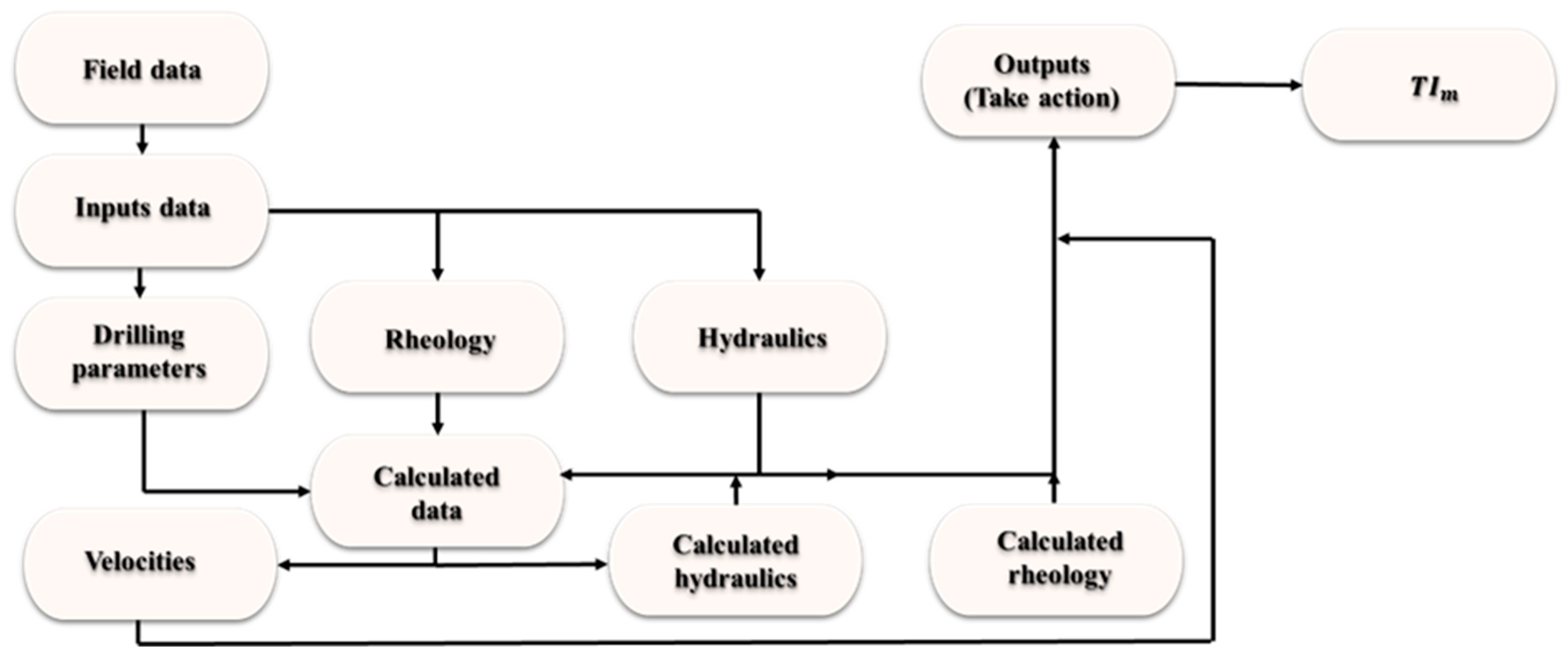Moreover, the cutting carrying index (CCI) provides knowledge of the size of cuttings, size of annulus, flow pattern, and down-borehole fluid properties that cannot be determined with a high degree of accuracy [13]. Considering the aforementioned details, the objective of this study is to present various indicators of borehole cleaning that can help determine the extent of borehole cleaning during the drilling of vertical, deviated, and horizontal wells. Additionally, the study aims to demonstrate how existing parameters can be used to develop a new transport index indicator (TI_m) for improving drilling performance and continuously monitoring and assessing borehole cleaning in real time during drilling. Figure 1 depicts the flowchart of the work.

Figure 1 demonstrates a comprehensive overview of the factors that can impact borehole cleaning, which are thoroughly examined in this study. The paper outlines various real-time models that serve as indicators for evaluating these factors as well as their respective limitations. Additionally, the mathematical development of the TI_m model is presented, which takes into account all relevant parameters necessary for evaluating the extent of hole cleaning in real time. The performance of the TI_m model is validated through field applications, highlighting its importance as a novel indicator model. Finally, the study concludes with insightful recommendations for future research in this field.

2. The Influence of Factors on Borehole Cleaning

The aim of borehole cleaning and cuttings transportation is to prevent cuttings from settling and to facilitate their rapid transport to the shale shaker. In addition to serving as a coolant for the bit, the mud’s primary role is to clean the drill bit face by removing and lifting cuttings away from it. Since the beginning of the studies on the cuttings transportation mechanism, one of the most important goals has been to obtain comprehensive knowledge about the process [28]. Identifying the specific factors affecting cuttings transportation is a difficult task as a single explanation that can satisfactorily explain all the gathered facts does not exist. However, a significant number of studies have arrived at the conclusion that the capacity of mud to transport rock pieces is dependent on the type of mud, its density and rheology, and the pace at which the mud flows or its annular velocity. In addition to the size and density of the cuttings, the borehole angle, RPM, ROP, and drill pipe eccentricity have an effect on cuttings transportation [10]. All the parameters that have an effect on cuttings transport are shown in Figure 2. As seen in Figure 2, it highlights the direct influence of variables such as borehole size and drilling fluid rheology, which can significantly enhance the cleaning process. However, there are also indirect factors, such as cutting size, density, shape, and the ROP, which can moderately impact borehole cleaning efficiency. Notably, certain variables can have a detrimental effect on the cleaning process. Inclinations, for instance, can pose a significant negative impact, making borehole cleaning efficiency difficult to achieve. On the other hand, there are factors that can significantly improve borehole cleaning conditions. Flow rate and RPM are examples of such variables, which can have a significant positive effect and optimize the cleaning process. It is therefore important to consider all the factors that can influence borehole cleaning conditions in order to achieve the best possible results [10,19].

In addition to these affects, the settling velocity of cuttings in drilling fluids is influenced by several parameters, including cuttings size, shape, and density, as well as drilling fluid density, viscosity, and velocity. Cuttings that are larger, denser, or irregularly shaped tend to settle more quickly than smaller, less dense, or rounded cuttings. The density of the drilling fluid plays a critical role in controlling the settling velocity of the cuttings, with higher density fluids suspending larger and denser cuttings more effectively [9,10]. The viscosity of the drilling fluid affects the drag force on the cuttings, slowing down their settling velocity, while the fluid velocity can affect cuttings suspension. The wellbore configuration and presence of confining walls, such as casing or formation, can also affect the settling velocity of cuttings. Finally, pipe rotation can create turbulence in the drilling fluid, helping to suspend the cuttings and reduce their settling velocity [9,29].

Moreover, this demonstrates that the eccentricity of the drill pipe has an indirect influence on cutting transport, but the size of the borehole, the characteristics of the mud, the amount of cuttings, and the flow rate all have direct impacts on the optimization of borehole cleaning. For example, when used in conjunction with other factors, rotation can boost borehole cleaning effectiveness even more (see Figure 3) [19,30,31]. Rotating the drill pipe can improve borehole cleaning by combining the rheology of the mud, the size of the cuts, and the flow velocity of the mud. Additionally, the dynamic behavior of the drill pipe, such as steady-state vibration, unsteady-state vibration, whirling rotation, and true axial rotation parallel to the borehole axis, can have a substantial impact on improving borehole cleaning. This is because the cuttings that have settled on the bottom side of the borehole will be stirred up into the top side when the borehole is rotated, which is where the flow is most efficient [32]. Figure 3 illustrates the effect that rotation has on the cutting bed at a variety of RPMs. The rotation of the pipe at low RPM demonstrates that the viscous coupling coating is of a thin thickness (Figure 3a). Figure 3b shows that when the pipe RPM is at a moderate level (medium RPM up to 100 RPM), the pipe begins to move up the borehole slightly, and the viscous coupling film starts to thicken, but it is still thinner than the tool joint upset. At a rotation speed of approximately 120 RPM, the pipe moves further up the borehole, and the thickness of the viscous coupling film reaches the height of the tool joint upset (Figure 3c). This can be explained by the fact that the fluid is no longer able to flow through the gap in a laminar fashion, leading to the formation of turbulent flow vortices that break off and stir the bed (Figure 3a) [10,33]. More importantly, if the viscosity of the drilling fluid is too high, the viscous coupling effect is very good, but the cuttings “dead zone” area decreases, and the fluid can only pass through the high velocity area of the wellbore, making the velocity dead zone too large, and the cuttings (Figure 3b). Moreover, it is impossible to enter the high velocity zone; if the viscosity of the DF is too low (Figure 3c), the ECD is very low, but the viscous coupling effect in the wellbore is very poor, and cuttings cannot be stirred into the conveyor belt, so the cleaning of the wellbore becomes more difficult [10,33,34].

The Main Models to Evaluate the Borehole Cleaning Efficiency

The efficiency of the borehole cleaning evaluation instruments and procedures is diminished if the findings are not received promptly. Addressing any borehole cleaning difficulties as soon as possible is essential to avoid a buildup of cuttings and the possibility of situations in which pipes have been trapped. The drilling crew is able to promptly evaluate borehole cleaning using real-time models and take corrective action, including modifying drilling fluid properties, adjusting surface parameters, or performing dedicated circulations to move cuttings to the surface. However, conventional rig sensors may not be capable of running some models on real time. Under such circumstances, incorporating sophisticated sensors and models may be necessary [10,17].

Hence, cuttings transport models based on experimental, mechanical, or field-applied approaches have been developed. As an example, the cutting carrying index (CCI) is an indicator that provides knowledge of the size of cuttings, size of the annulus, flow pattern, and downhole fluid properties that cannot be determined with a high degree of accuracy. Leon Robinson developed a simple empirical index to help predict borehole cleaning [13]. When the cuttings are effectively lifted to the surface, the product of the three key variables that have a significant impact on the transport ratio is approximately 400,000. The presence of sharp-edged and well-defined cuttings is a reliable indication of good borehole cleaning [13]. If the edges are rounded, tumbling occurs in the annulus, which means that cuttings are not transported to the surface quickly. A borehole cleaning index or ratio of 1 or greater is considered indicative of good borehole cleaning conditions. When the CCI value is 0.5 or less, the cuttings are more rounded and smaller due to inefficient borehole cleaning, which leads to a longer residence time in the annulus. This CCI is applicable for vertical borehole sections with inclinations ranging from 0 to 25 degrees [13]. For deviated and horizontal borehole sections, CCI must be modified. Another model that allows us to indicate the amount of cuttings beds removed by determining their critical height is called the borehole cleaning ratio (HCR) [27]. An HCR value greater than 1 indicates that the drilling fluid is removing cuttings effectively and maintaining a clean wellbore. On the other hand, an HCR value of less than 1 indicates that the cuttings are settling in the wellbore and not being effectively removed [27]. More importantly, every model performs by considering the influence of different parameters on the obtained results.

Table 1. Various models indicating the cutting transport or borehole cleaning conditions.

№	Name of Model	Equations	Definition	Ref.
1	Hole cleaning ration (HCR)	$\mathrm{H}\mathrm{C}\mathrm{R}=\frac{{\mathrm{H}}_{\mathrm{r}}}{{\mathrm{H}}_{\mathrm{c}\mathrm{r}\mathrm{i}\mathrm{t}}}$	The HCR is a ratio between the free height of the drilling fluid in the annulus and the critical height of the cuttings bed, and it is commonly utilized to assess the risk of a pipe becoming stuck during drilling operations.	[27]
2	$\mathrm{Cutting} \mathrm{carrying} \mathrm{index} (\mathrm{C}\mathrm{C}\mathrm{I}$)	$\mathrm{C}\mathrm{C}\mathrm{I}=\frac{\mathrm{M}\mathrm{W} \mathrm{K} \mathrm{V}\mathrm{a}\mathrm{n}\mathrm{n}}{\text{400,000}}$	$\mathrm{The} \mathrm{C}\mathrm{C}\mathrm{I}$ is used to indicate the borehole cleaning efficiency in vertical borehole sections.	[13]
3	$\mathrm{Cutting} \mathrm{concentration} \mathrm{in} \mathrm{annulus} \left({\mathrm{C}\mathrm{C}\mathrm{A}}_1\right)$	${\mathrm{C}\mathrm{C}\mathrm{A}}_1=-\frac{1}{2}\left(\frac{{\mathrm{V}}_{\mathrm{a}\mathrm{n}\mathrm{n}}}{{\mathrm{V}}_{\mathrm{s}}}-1\right)+(\frac{1}{4}{\left(\frac{{\mathrm{V}}_{\mathrm{a}\mathrm{n}\mathrm{n}}}{{\mathrm{V}}_{\mathrm{s}}}-1\right)}^2{+\frac{{\mathrm{V}}_{\mathrm{a}\mathrm{n}\mathrm{n}}}{{\mathrm{V}}_{\mathrm{s}}}\frac{\mathrm{V}\mathrm{c}}{\frac{\mathrm{G}\mathrm{P}\mathrm{M}}{7.48}})}^{0.5}$	$\mathrm{The} {\mathrm{C}\mathrm{C}\mathrm{A}}_1$ is commonly utilized to assess the cessation of circulating during connections and the circulation which occurs prior to a connection.	[35]
4	$\mathrm{Cutting} \mathrm{concentration} \mathrm{in} \mathrm{annulus} \left({\mathrm{C}\mathrm{C}\mathrm{A}}_2\right)$	$\frac{1}{{\mathrm{C}\mathrm{C}\mathrm{A}}_2}=1+\left(1-\frac{\mathrm{O}{\mathrm{D}}^2}{\mathrm{O}{\mathrm{H}}^2}\right)\left(\frac{\mathrm{V}\mathrm{a}\mathrm{n}\mathrm{n}-\mathrm{V}\mathrm{s}}{30}\right)(\frac{1800}{\mathrm{R}\mathrm{O}\mathrm{P}}+\frac{\mathrm{V}\mathrm{s}}{\frac{24.5\mathrm{G}\mathrm{P}\mathrm{M}}{\mathrm{O}\mathrm{H}-\mathrm{O}\mathrm{D}\mathrm{c}}-\mathrm{V}\mathrm{s}}\mathrm{T}\mathrm{c})$	The ${\mathrm{C}\mathrm{C}\mathrm{A}}_2$ is commonly utilized to assess the steady state lifting solids in the vertical tube.	[8]
5	$\mathrm{Transport} \mathrm{ratio} (\mathrm{T}\mathrm{R}$)	$\mathrm{T}\mathrm{R}=\frac{\mathrm{V}\mathrm{a}\mathrm{n}\mathrm{n}-\mathrm{V}\mathrm{s}}{\mathrm{V}\mathrm{a}\mathrm{n}\mathrm{n}}$	$\mathrm{The} \mathrm{T}\mathrm{R}$ is used to evaluate the efficiency with which cuttings are removed from the wellbore.	[36]
6	$\mathrm{Lifting} \mathrm{coefficient} ({\mathsf{\beta }}^1$)	${\mathsf{\beta }}^1=0.11519·\frac{Q_m}{A_a}·{(1-C_f)}^{-1}·{\left(d_c\right)}^{-2.014}$	$\mathrm{The} {\mathsf{\beta }}^1$ is utilized to evaluate the borehole cleaning attributes for optimal cuttings lifting ability and cuttings lifting coefficient, both of which provide requirements for cutting lifting in a wellbore.	[17]
7	$\mathrm{Transport} \mathrm{index} (\mathrm{T}\mathrm{I}$)	$\mathrm{T}\mathrm{I}=\frac{GPM·RF·MW}{100}or=RF·AF·MW$	$\mathrm{The} \mathrm{T}\mathrm{I}$ is used to evaluate the effectiveness of the drilling fluid in removing cuttings and maintaining a clean wellbore.	[37]

shows various models to indicate the cutting transport or borehole cleaning conditions.

As seen from Table 1, each model has specific set of variables that are crucial in assessing different aspects of drilling operations. For instance, the HCR is commonly used to evaluate the risk of a pipe becoming stuck during drilling operations by calculating the ratio between the free height of the drilling fluid in the annulus and the critical height of the cuttings bed [27]. Similarly, the CCI is based on other variables such as mud weight, consistency factor, and annular velocity, and is used to evaluate the ability of the drilling fluid to transport cuttings out of the wellbore. The TR model, on the other hand, is used to assess the efficiency of cuttings removal based on annular velocity and slip velocity [13]. Additionally, the ${\mathsf{\beta }}^1$ model is utilized to evaluate the borehole cleaning attributes for the optimal cuttings lifting ability and cuttings lifting coefficient based on the drilling fluid flow rate, annular area, and cutting diameter [17]. However, among these models, the TI model stands out due to its incorporation of various variables such as mud weight, rheology factor, flow rate, and angle factor, which are crucial in evaluating the overall borehole cleaning efficiency during drilling operations [37].

More importantly, there are several models, tools, chemicals, charts, methodologies and correlations that were used; however, they were not applicable, inefficient, costly, and not feasible with drilling operations such as ${\mathrm{C}\mathrm{C}\mathrm{A}}_1$ [35]. Moreover, the models utilized to assess the drilling performance and the borehole cleaning conditions have several significant inadequacies. First, they do not consider the mud weight in both static and dynamic conditions, including equivalent circulating density. Second, there are other critical factors that they do not consider, including hydraulic velocities, rheological properties of drilling fluids (including the low shear yield point), flow regime, and cuttings properties, which can all have an impact on the drilling process. In summary, each model provides a unique perspective on evaluating the cutting transport and borehole cleaning conditions during drilling operations, with the TI model being the most comprehensive and inclusive among them. Addressing these shortcomings can lead to more accurate and reliable predictions, ultimately improving the safety and efficiency of drilling operations.

Therefore, in the next section, we present a newly developed model called the transport index based on Luo’ 1992 and 1994 [37,38], which provides a comprehensive evaluation of various factors impacting borehole cleaning. The novel model is designed to assist drilling teams in optimizing drilling operations by empowering them to make informed decisions about necessary modifications based on a thorough understanding of the underlying factors. By utilizing the novel model, drilling teams can identify potential issues and make necessary modifications in a timely and efficient manner, ultimately leading to improved safety, efficiency, and cost effectiveness. This model is particularly valuable in reducing the need for expensive additives and chemicals in the drilling fluid system, which can significantly impact the overall cost of drilling operations.

3. Mathematical Development of the Model for the TI_m

The transport index is a model used in drilling operations to evaluate the effectiveness of the drilling fluid in removing cuttings and maintaining a clean wellbore. It is a measure of the ability of the fluid to transport cuttings out of the wellbore and to the surface and was developed by Luo in 1992 [37,38]. The first model is described by the following Equation [37]:

$$\mathrm{T}\mathrm{I}=\frac{GPM·RF·MW}{100}$$

(1)

where GPM is the flow rate of the mud pump (gal/min), RF is the rheology factor, and $MW$ is the static drilling fluid density (lb/cf).

RF was added to Equation (1) to describe the combined effect of the PV and YP of drilling fluids on fluid rheology.

Moreover, Luo proved that the penetration rate depends on the mud weight, flow rate, and the rheology factor. As seen in Figure 4, from the chart, the TI and borehole angle can be applied to determine the maximum ROP while drilling based on the results obtained from Equation (1) [37].

More importantly, in 1994, Luo showed a straightforward graphical approach that could be used on the rig to evaluate borehole cleaning for different sized boreholes. The model employs a series of charts to assess the efficacy of the borehole cleaning procedure [38]. The full model was obtained by combining the effects of the mud weight (MW), angle factor (AF), and rheology factor (RF), as shown in Equation (2) [38].

$$\mathrm{T}\mathrm{I}=RF·AF·MW$$

(2)

Based on [37,38], using Equations (1) and (2), a series of charts were developed for each of the borehole diameters to calculate the value of the RF based on the mud PV and YP. A higher RF value indicates a mud that is more viscous and thicker, which translates to better suspension of cuttings and more efficient transport to the surface [10]. As an example, Figure 5 shows the RF for the borehole size 17–12″.

From Equations (1) and (2), the AF is a term used in directional drilling to describe the effect of the borehole angle on the amount of cuttings that can be transported by the drilling fluid. A higher wellbore angle can result in a lower AF value, indicating that borehole cleaning may become more difficult. The AF can be obtained based on the borehole angle, as shown in

Table 2. Angle factor values at different borehole angles.

AF by Luo [38]		AF by Unegbu [21]
Borehole Angle	Angle Factor	Borehole Angle	Angle Factor
0	-	0	2.03
25	1.51	25	1.51
30	1.39	30	1.39
35	1.31	35	1.31
40	1.24	40	1.24
45	1.18	45	1.18
50	1.14	50	1.14
55	1.1	55	1.1
60	1.07	60	1.07
65	1.05	65	1.05
70–80	1.02	70	1.02
80–90	1	80	1

[38]. More importantly, Unegbu developed a model based on the flow rate in 2010 to determine the equivalent RF based on the borehole angle for vertical and deviated wells, as shown in Table 2 [21].

Despite the fact that the model was able to evaluate the borehole cleaning conditions in real time, Luo’s model considers only the mud weight in static conditions, flow rate, and rheology factor. Moreover, the RF can only be obtained from the chart, which also depends on the borehole size [37,38]. The AF can only be obtained from Table 2 [21,37,38]. Therefore, the main novelty of the novel modified model transport index (${TI}_m)$ is to consider the MW in static and dynamic conditions (ECD), develop a new model by interpolation to calculate the AF at any borehole angle, and develop a novel model to calculate the RF. More importantly, the novel ${TI}_m$ model considers a range of additional factors, including hydraulic velocities, the rheological characteristics of the drilling fluids with regard to the low shear yield point (LSYP), the flow regime, the properties of the cuttings, and ECD [39]. Moreover, ${TI}_m$ is an automated indicator based on two criteria to evaluate real-time borehole cleaning during drilling operations. If the value of ${TI}_m$ is above 1, borehole cleaning is satisfactory. On the other hand, if ${TI}_m$ falls below 1, borehole cleaning is inadequate. In essence, the ${TI}_m$ model provides an easy-to-use indicator of the efficiency of the drilling process in removing cuttings and maintaining a clean wellbore. By using this model, drilling operators can quickly assess the state of borehole cleaning and take corrective measures and actions if necessary [21,37,38].

Accordingly, the novel modified model transport index (${TI}_m)$ was developed based on the effective mud weight ${(MW}_{eff}$) calculated using Equation (1) [8].

$${MW}_{eff}=MW·CCA+MW$$

(3)

where the variable CCA represents the cuttings concentration in an annulus, and it is defined by Equation (4) [8,40].

$$CCA or {CCA}_{API}=\frac{ROP{ · OH}^2}{1471·GPM·TR}$$

(4)

where ROP represents the rate of penetration (ft/h), OH represents the diameter of the borehole size (inch), and 1471 is a conversion factor. GPM represents the pump flow rate in gal/min, and TR represents the transport ratio. The transport ratio can be substituted with a value of 0.55 according to [8]. From Equation (3), in real time, the ECD can be found based on ${MW}_{eff}$ (pcf). Specifically, Equation (4) can be used to determine the ECD [39].

$$ECD=MW+\left(\left(\frac{0.085}{OH-{OD}_{pipe}}\right)·\left(\mathrm{Y}\mathrm{P}+\frac{PV Vann}{300(OH-{OD}_{pipe})}\right)\right)·7.481$$

(5)

where $PV$ is the plastic viscosity (cP), and $YP$ is the yield point (lb/100 sqft). The LSYP refers to the amount of force required to initiate fluid movement in the wellbore, and it plays a critical role in ensuring that the drilling fluid can effectively suspend and transport cuttings out of the wellbore. Therefore, it is important to consider the LSYP in conjunction with PV and YP to ensure that the drilling fluid system is optimized for efficient and safe drilling operations. ${PV}_m$ and ${YP}_m$ can be modified based on the LSYP, as shown in Equations (6) and (7).

$${PV}_m=\left(R600-LSYP\right)-\left(R300-LSYP\right)$$

(6)

$${YP}_m=2\left(R300-LSYP\right)-(R600-LSYP)$$

(7)

where R600 represents the Fann reading viscometer at 600 RPM, and R300 represents the Fann reading viscometer at 300 RPM. Accordingly, the PV and YP are replaced in the forward Equations with ${PV}_m$ and ${YP}_m$.

More importantly, $k$ and $\mathrm{n}$ are the consistency factor (cP) and the flow behavior index, respectively. The values of k and n must be optimized for the specific drilling conditions to ensure effective borehole cleaning. If the values of k and n are not carefully monitored and adjusted, the drilling fluid may struggle to suspend and transport cuttings out of the wellbore, leading to significant operational challenges. Therefore, it is crucial to carefully monitor and adjust the values of k and n for the drilling fluid system to ensure optimal borehole cleaning efficiency. Therefore, $k$ and $n$ can be further modified based on LSYP, which equals (LSYP = 2R3 − R6) in accordance with [41,42] to consider the viscometer reading at 600 RPM, 300 RPM, 200 RPM, and 100 RPM. Moreover, $k$ and n can be obtained by considering the reading of the viscometer at 6 RPM and 3 RPM for a pipe and an annulus [41,42,43]. $k_m$ and $n_m$ can be obtained from Equations (8) and (9), respectively.

$$k=\frac{510·R_{300}}{{511}^n}=k_m=\frac{{510·(0.5·(R}_{300}+R_{100}\left)\right)-LSYP}{{511}^{n_m}}$$

(8)

$$n=3.32·log\left(\frac{R_{600}}{R_{300}}\right)=n_m=3.32·log\left(\frac{{0.5·(R}_{600}+R_{200})-LSYP}{{0.5·(R}_{300}+R_{100})-LSYP}\right)$$

(9)

In particular, Newit developed a more accurate CCA model for steady-state lifting of materials in a vertical tube by using Equation (4), which may be found in Equation (10) [8,35]. Mitchell provided evidence that an annular concentration model may be derived by taking into account both the circulation that takes place before a connection but after drilling has been halted and the circulation that takes place after connections but before drilling resumes. The time known as the preconnection circulation period is what is known as the later circulation. The annulus is where his Equation tells us to go and obtain the average cutting volume percent that was computed for us (see Equation (11)) [8].

$${CCA}_1=-\frac{1}{2}\left(\frac{{Vann}_m}{V_{sa}}-1\right)+{\left(\frac{1}{4}{\left(\frac{{Vann}_m}{V_{sa}}-1\right)}^2+\frac{{Vann}_m}{V_{sa}}\frac{Vc}{\frac{GPM}{7.48}}\right)}^{0.5}$$

(10)

$${CCA}_2=\frac{1}{1+\left(1-\frac{OD}{OH}\right)\left(\frac{{Vann}_m - V_{sa}}{30}\right)(\frac{1800}{1 + ROP}+\frac{V_{sa}}{V_{ann.dc} - V_{sa}}·T_{PC})}$$

(11)

where ${Vann}_m$ represents the annular modified velocity of the drilling fluid (ft/min) (Equation (12)), $V_{ann.dc}$ is the annular velocity across the drill collar (ft/min), $T_{PC}$ is the preconnection circulation time, which specifies the amount of time required to circulate the cuttings to a height that will prevent them from sinking to the bottom of the borehole during the process of making that connection (min), $V_{sa}$ is the average velocity of cutting slip (ft/min), and $V_c$ is the volumetric rate of cuttings entering the annulus (ft/min). ${Vann}_m$, $V_{ann.dp}$, $V_{ann.dc}$, $T_{PC}$, $Vc$, and $V_{sa}$ can be obtained from Equations (12)–(17), respectively.

$$\begin{array}{c}{V}_{ann.m}=\frac{24.5GPM}{{OH}^2-{{OD}_{pipe}}^2}=\hfill \\ =(\frac{24.5·GPM}{{OH}^2-{{OD}_{pipe}}^2}cos(\alpha )\hfill \\ +\left(\frac{60}{\left(1-{\left(\frac{{OD}_{pipe}}{OH}\right)}^2\right)·\left(0.64+\frac{18.2}{ROP}\right)}+\frac{ROP\left(O{H}^2\right)}{60\left(O{H}^2-{{OD}_{pipe}}^2\right)}\right)\mathit{sin}\left(\beta \right))\hfill \\ -\frac{175\left(d_{cm}\right){\left(\frac{Wc}{7.481}-\frac{{MW}_{eff}}{7.481}\right)}^{2n_m}}{\left({MW}_{eff}{/7.481)}^{n_m}\right(\frac{2.4 · V_{ann.dp}}{OH - {OD}_{pipe}}·\left(\frac{2n_m + 1}{3n_m}\right)·\left(\frac{200K_m\left(OH - {OD}_{pipe}\right)}{V_{ann.dp}}\right){)}^{n_m}}\hfill \end{array}$$

(12)

$$V_{ann.dp}=\frac{24.5\left(GPM\right)}{{OH}^2-{{OD}_{pipe}}^2}$$

(13)

$$V_{ann.dc}=\frac{24.5\left(GPM\right)}{{OH}^2-{{OD}_c}^2}$$

(14)

$$T_{PC}=\frac{V_{sa}}{V_{ann.m}-V_{sa}}·T_C$$

(15)

$$Vc=\frac{ROP·{OH}^2}{1100}$$

(16)

$$V_{sa}=\frac{V_{sm}+V_{sc}}{2}$$

(17)

where $\alpha$ is the borehole angle (degrees), $\beta$ is the azimuth angle (degrees), $T_C$ refers to the time for making the connection (min), $V_{ann.dp}$ is the annular velocity across the drill pipe (ft/min), ${OD}_c$ represents the outer diameter of the drill collar, $V_{cr}$ is the cutting rise velocity(ft/min), $V_{sc}$ is the cutting slip velocity due to ROP which equals ${{(V}_{sc}=V_{ann}-V}_{cr}$) (ft/min) in accordance with [43], and $V_{sm}$ is the slip velocity considering the flow regime (ft/min) based on [44]. The $V_{sm}$ includes the cutting velocities calculated based on the weight of the cuttings, the effective viscosity of the drilling fluid, and the rate of penetration [41,44,45,46]. More importantly, Hopkin also showed that the mud weight ($F_m$) can affect the speed of slipping, and he developed Equation (18) [47]. Therefore, the new average slip velocity with considering the influence of mud weight ($V_{sm.n}$) can be obtained from Equation (21). Furthermore, Equation (21) shows that $V_{s1}$ and $V_{s2}$ represent the velocities that are determined by taking into account the effective viscosity, apparent viscosity, weight, and diameter of the cuttings, which are also considered in Equations (19) and (20).

$$F_m=\left(2.117-\frac{0.1648{MW}_{eff}}{7.481}+0.003681{\left(\frac{{MW}_{eff}}{7.481}\right)}^2\right)$$

(18)

$$V_{s1}=0.45\left(\frac{M_{eff}}{\left(\frac{{MW}_{eff}}{7.481}{d}_{cm}\right)}\right){\left(\left(\frac{\text{36,800} {MW}_{eff}{d_{cm}}^3\left(\frac{Wc}{7.481}-\frac{{MW}_{eff}}{7.481}\right)}{{M_{eff}}^2}\right)+1\right)}^{0.5}-1$$

(19)

$$V_{s2}=\left(\frac{175\left(d_{cm}\right){\left(\frac{Wc}{7.481}-\frac{{MW}_{eff}}{7.481}\right)}^{0.667}}{{{MW}_{eff}}^{0.333}Map{p}^{0.333}}\right)$$

(20)

$$V_{sm.n}=\frac{V_{s1}+V_{s2}}{2}·F_m\to V_{sa}=\frac{V_{sm.n}+V_{sc}}{2}$$

(21)

In Equations (19) and (20), $d_{cm}$ is the modified cutting diameter (inches), $Wc$ is the cuttings density (lb/cf) according to [17,48], $M_{eff}$ is the effective viscosity of the drilling fluid (cP), and $Mapp$ is the apparent viscosity of the drilling fluid (cP), which can be obtained from Equations (22)–(25), respectively.

$$Wc=\left({MW}_{eff}CCA+{MW}_{eff}\right)+\left(1-CCA\right){MW}_{eff}$$

(22)

$$d_{cm}=0.2·\frac{ROP}{RPM+xGPM}$$

(23)

$$M_{eff}={PV}_m+{300YP}_m·\frac{d_{c.m}}{V_{ann.m}}$$

(24)

$$Mapp={\left(\left(\frac{2.4·V_{ann.dp}}{OH-OD}·\left(\frac{2n_m+1}{3n_m}\right)(\frac{200K_m\left(OH-OD\right)}{V_{ann.dp}}\right)\right)}^{n_m}$$

(25)

Hence, the modified ${CCA}_{am}$ described by Equation (26) takes all the affecting factors and the velocity of annular cuttings for the drill collar, the drill pipe, and the connection time into account [8].

$${CCA}_{am}=\frac{{CCA}_{API}+{CCA}_1+{CCA}_2}{3}$$

(26)

More importantly, Pejcinovic et al. modified the consistency index and flow behaviour index defined by Equations (8) and (9), respectively, to incorporate the effects of rheological properties by including the concentration of solids based on the power law model. The results show that k increases with increasing solid concentration, while n decreases [49]. The solid concentration can be referred to as the concentration of cuttings in the annulus. Thus, the modified consistency index ($k_{e.m}$) and ($n_{em}$)-based CCA_m can be obtained from Equation (27).

$$k_{e.m}={K_m}^{{CCA}_{am}} and the n_{em}={n_m}^{-{CCA}_{am}}$$

(27)

As seen in Equation (2), ${\mathrm{R}\mathrm{F}}_1$ can be obtained and modified according to the Unegbu’s model based on CCI and TR [21]. CCI can be equal to $TR$ according to Equations (28) and (29) [21]. Moreover, $Vann$ in Equation (28) can be replaced by its definition in Equation (30). Thus, ${RF}_1$ can be obtained from Equation (31) by considering the modified $k_{e.m}$ from Equation (27).

$$CCI=\frac{MW K Vann}{\text{400,000}}$$

(28)

$$TR=\frac{GPM MW RF}{834.5}$$

(29)

$$Vann=\frac{24.5GPM}{{OH}^2-{{OD}_{pipe}}^2}$$

(30)

$${RF}_1=\frac{K}{146.4·{(OH}^2-{{OD}_{pipe}}^2)}=\frac{k_{e.m}}{146.4·{(OH}^2-{{OD}_{pipe}}^2)}$$

(31)

Furthermore, based on [21,50,51,52], to include the effects of the temperatures and ${CCA}_{am}$, ${RF}_2$ can be computed using Equation (32). Thus, the average modified ${\mathrm{R}\mathrm{F}}_{\mathrm{a}\mathrm{m}}$, incorporating the effects of temperatures and ${CCA}_{am}$, is defined by Equation (33)

$${RF}_2=0.5·\left(\frac{{PV}_m}{{YP}_m}+\frac{{YP}_m}{{PV}_m}\right)·\left(1-\frac{T_2}{T_1}·{CCA}_{am}\right)$$

(32)

where T₂ is the borehole temperature, and T₁ is the flow line temperature at the surface.

$${RF}_{av}=\frac{{RF}_1+{RF}_2}{2}$$

(33)

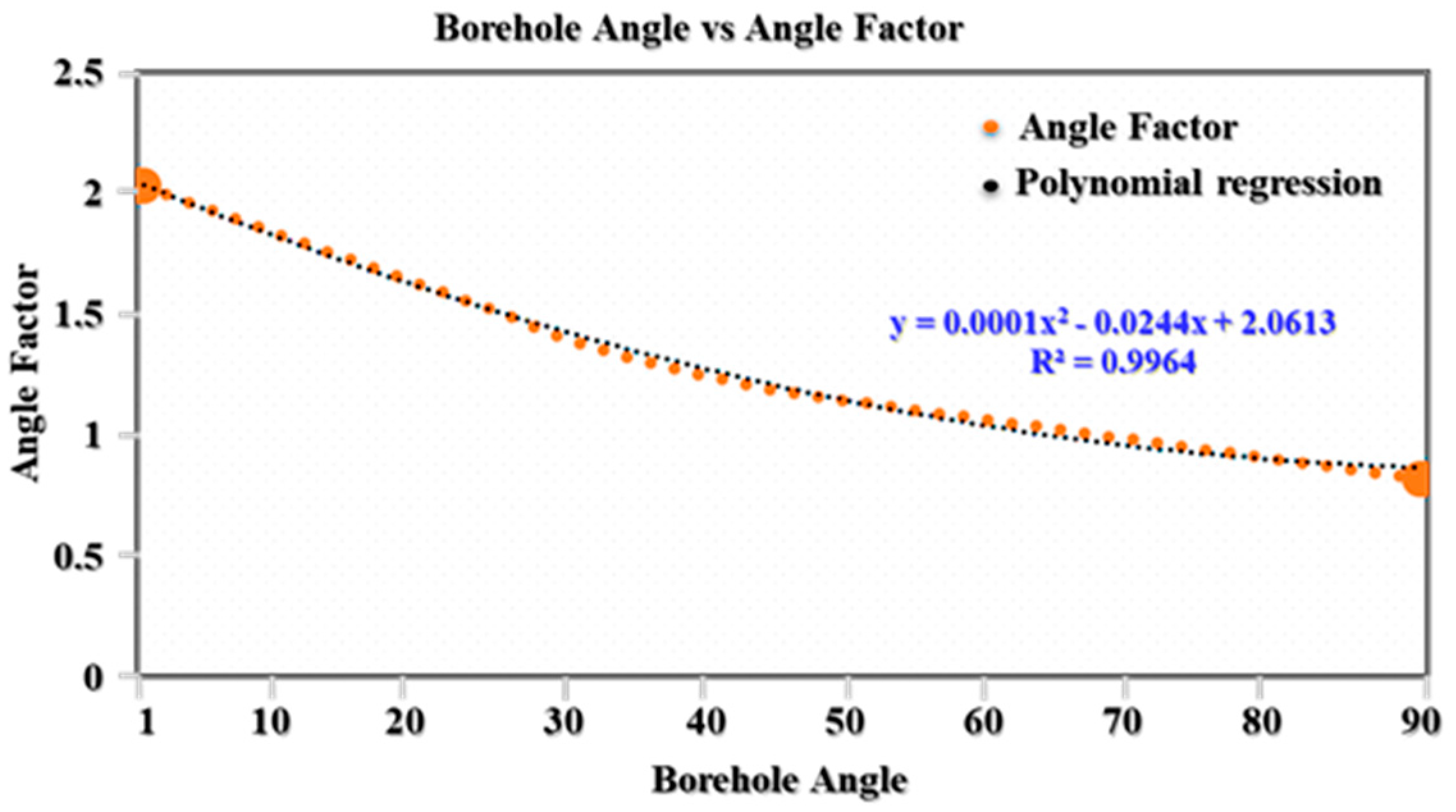
Moreover, from Equation (2) and based on Unegbu’s model [21], AF was found in accordance with Table 2 based on the changes in the borehole angle [21,37,38]. Accordingly, AF was modified, and a new model was developed by interpolation to calculate AF at any borehole angle (see Figure 6). As shown in Equation (34), the AF regime is characterized by two important parameters: the α borehole angle and ${CCA}_{am}$. The α borehole angle represents the angle between the wellbore axis and the horizontal plane and ${CCA}_{am}$ is a critical parameter that impacts the ability of the drilling fluid to effectively transport cuttings out of the wellbore. Hence, the AF regime and the parameters associated with it must be carefully monitored and evaluated to ensure optimal borehole cleaning efficiency [21,37,38]. Figure 6 shows the interpolation of the AF based on the borehole angle.

$$\begin{gathered} {AF}_m=-0.0208\alpha +2.03 \\ Or \\ (0.0001{\left(\alpha \right)}^2-0.03\left(\alpha \right)+2.1)(1-{CCA}_{am}) \end{gathered}$$

(34)

More importantly, it is important to take into consideration real-time drilling factors such as the density of the cuttings, the weight of the drilling fluid, and the rheology of the drilling fluid [53]. Furthermore, ${ECD}_m$ can be obtained from Equation (35) using parameters defined by Equations (5)–(9). Moreover, MW defined by Equation (3) can be obtained using the original lifting capacity (LC) as shown in Equation (36) [53] and be modified (${LC}_m$). Furthermore, ${LC}_m$ can be included in ${RF}_{av}$ to incorporate the influence of bouncy on rheology in accordance with [53].

$$\begin{array}{ccc}\hfill {ECD}_m={MW}_{eff}& +& {\displaystyle (}\left(\frac{0.085}{OH-{OD}_{pipe}}\right)\hfill \\ \hfill & ·& {\displaystyle (}\left(2R300-LSYP\right)-\left(R600-LSYP\right)\hfill \\ \hfill & +& \frac{(\left(R600-LSYP\right)-\left(R300-LSYP\right))Vann.m}{300(OH-{OD}_{pipe})}{\displaystyle )}{\displaystyle )}·7.481\hfill \end{array}$$

(35)

$$LC=\frac{MW}{Wc}\to {LC}_m=\frac{{MW}_{eff}}{Wc}$$

(36)

As a direct result, Equation (37) may be applied to compute and finally determine the updated TI_m:

$$\begin{array}{ccc}\hfill {TI}_m=MW·{(RF}_{av}& +& {LC}_m)·{AF}_m\hfill \\ \hfill & =& \left(\frac{{MW}_{eff}}{{ECD}_m}\right)\left(\frac{{RF}_1+{RF}_2}{2}+\left(\frac{{MW}_{eff}}{Wc}\right)\right)·\left(-0.0208\alpha +2.03\right)\hfill \end{array}$$

(37)

where MW is the specific gravity of the used drilling fluids, which can be computed as SG = $MW/62.4$, (pcf).

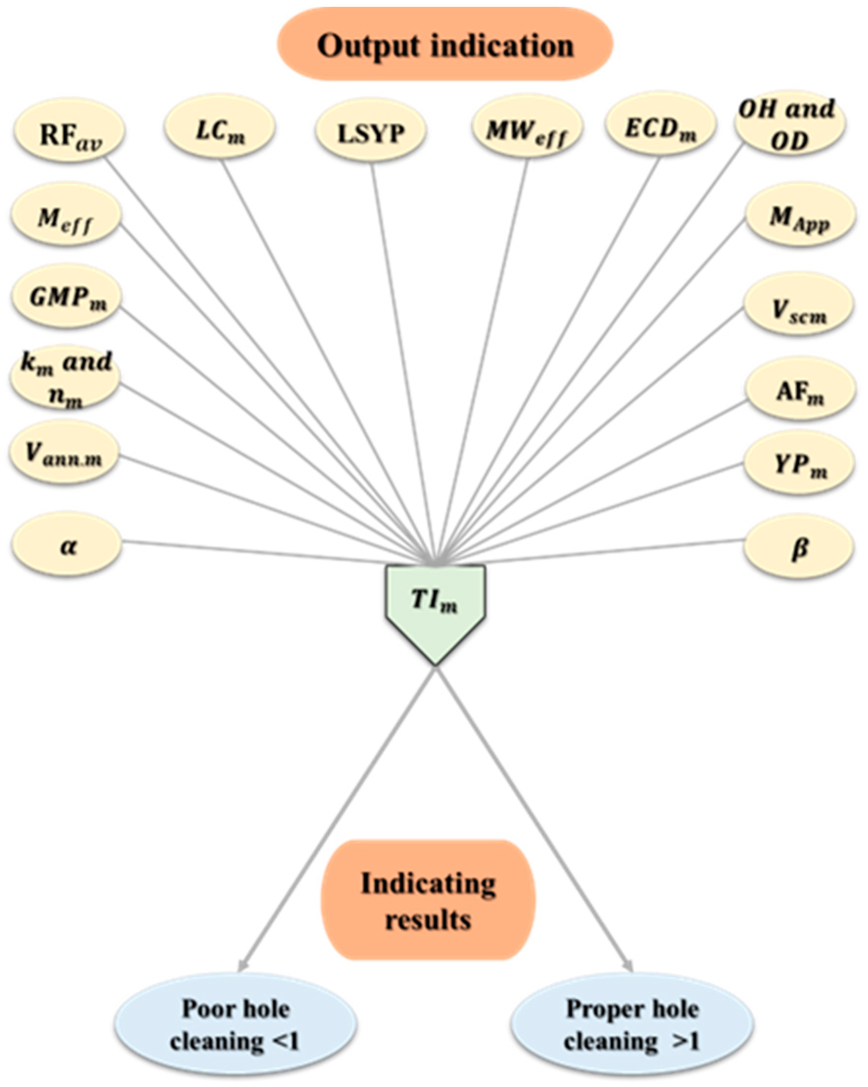
The development of a novel ${TI}_m$ model represents a significant advancement in drilling operations. The model contains different parameters, such as hydraulic velocities, rheological characteristics of drilling fluids (including the low shear yield point, k and n factor based on CCA_m), flow regime, cuttings properties such as diameter and weight, ECD, lifting capacity, and angle factor, to create a unique ${TI}_m$ model. As depicted in Figure 7, initial parameters such as CCA and MW_eff can be used to determine ${TI}_m$. The ${TI}_m$ model provides a reliable indication of the state of borehole cleaning, and two different standards are applied to judge the performance of the model for evaluating the conditions of borehole cleaning. A ${TI}_m$ value of more than 1 indicates that the borehole cleaning process was carried out correctly, while a ${TI}_m$ value of less than 1 indicates unsatisfactory borehole cleaning in accordance with [21,37,38].

4. Results and Discussion

4.1. Methodology

In this study, the TI_m model was rigorously validated through the directional drilling of intermediate sections in two offshore wells and a horizontal section in a third well. Specifically, the model was evaluated for the drilling of the 12.25″ intermediate sections and horizontal sections in Well-A and Well-B, as well as the 8.5″ liner section in Well-C, which presented a challenge due to stuck pipe. These deviated drilling sections were severely deviated, with the first two starting at 30 degrees and the third achieving a near-horizontal inclination of 90 degrees with respect to the borehole at the top of the reservoir in Well-A and Well-B. The third well was horizontally drilled at 90 degrees. In this study, properties of the formation and drill cuttings were carefully considered to ensure the effectiveness of the drilling process. The formation was composed of sandstone, limestone, and shale, with formation temperatures ranging from 140 to 155 °F. The porosity of the formation ranged from 0.15 to 0.25. The washout, which is the enlargement of the wellbore diameter due to the erosion of the formation, ranged from 10% to 30%. The properties of the drill cuttings are also critical to the success of the drilling process. The density of the drill cuttings ranged from 20 to 24 ppg. The size of the drill cuttings ranged from 0.2 to 0.375 inches.

Table 3. Drilling fluid properties.

Parameter	The Drilling Fluids Range Properties
The density of oil-based drilling fluid density	80 lb/ft3 for Well-A and Well-B 88-lb/ft3 for Well C
The ratio of oil	(0.7–0.8)
The ratio of water	(0.2–0.3)
The value of electrical stability	(500–1000) V
Percent of low gravity solids	(2–6) (%)
Percent of high gravity solids	(9–16) (%)
March funnel viscosity	(55–80) (s)
Percent of solid content	(10–15) (%)
Mud solid control	0.4–0.55

summarizes the properties of the drilling fluid used to drill these sections.

Other important parameters in addition to the properties of the formation and drill cuttings were also carefully monitored and recorded during the drilling operations. These parameters include the rheological properties of the drilling fluid, mechanical drilling parameters, borehole section directional survey, and hydraulic velocities. The accurate determination and tracking of these parameters were necessary for the calculation of TI_m. To facilitate analysis and interpretation of the data, tables were created to summarize the various parameters recorded during drilling operations.

Table 4. The parameters determined for Well-A.

Main Parameters	Minimum	Maximum	Average
α	30	90	60
β	69	110	90
MW	80	80	80
PV	31	32	31.5
YP	23	24	23.5
R3	12	13	13.5
R6	13	14	13.5
WOB	10	40	24.5
RPM	49	177	153.6
GPM	590	1033	958
SPP	898	2729	2411

summarizes the rheological properties of the drilling fluid for Well-A,

Table 5. The parameters determined for Well-B.

Main Parameters	Minimum	Maximum	Average
α	30	90	60
β	55	145	98.3
MW	80	80	80
PV	30	30	30
YP	23	23	23
R3	11	11	11
R6	8	8	8
WOB	22	40	30
RPM	50	190	170
GPM	642.2	688.78	686
SPP	1500	3004	2740

summarizes those for Well-B, and

Table 6. The parameters determined for Well-C.

Main Parameters	Minimum	Maximum	Average
α	22.9	90	75.5
β	88	120	110
MW	88	88	88
PV	19	29	24.5
YP	20	24	20.7
R3	7	9	8.5
R6	9	11	9.8
WOB	0	38	27
RPM	42	103	78.5
GPM	272	778	565
SPP	1060	4420	3934

summarizes those for Well-C. The mechanical drilling parameters and borehole section directional survey data for each well were also included in their respective tables. The hydraulic velocities were also recorded to ensure effective removal of drill cuttings from the wellbore. These data were crucial for the calculation of TI_m, which required accurate and up-to-date information on the position and orientation of the drill bit.

More importantly, a total of 2512 data points were collected to evaluate and study the performance of the novel TI_m model with different drilling parameters from various types of drilling fluids, including oil-based drilling fluids, water-based drilling fluids, inverted emulsion drilling fluids, and synthetic drilling fluids. The data were collected from different types of profile wells, including vertical, deviated, and horizontal wells.

4.2. Effects of Parameters of the Drilling Fluids on the Novel Model TI_m

The performance of the novel TI_m as an automated real-time indicator during drilling was evaluated based on various drilling fluid parameters. The drilling fluid properties play a crucial role in effective drilling operations and can greatly impact the performance of the TI_m [50,51,52]. Thus, the performance of TI_m was comprehensively evaluated by analysing a diverse range of drilling fluid types and well profiles. The results in Figure 8a clearly show that the performance of TI_m is enhanced as M_Weff increases, indicating that drilling fluids with a higher density can improve the borehole cleaning capability and enhance the performance of TI_m. A drilling fluid with a higher density enhances the borehole cleaning due to its ability to carry more solids and cuttings out of the wellbore. On the other hand, Figure 8b shows that the higher the ECD, the lower the TI_m performance. This indicates that the TI_m model can be effectively used to evaluate borehole cleaning during drilling in real time. Figure 8c shows that the performance of TI_m increases with increasing LC_m. This indicates that the TI_m model can be used to accurately evaluate the performance of drilling operations in terms of the amount of cuttings being removed from the wellbore [54].

The results in Figure 9a clearly show that the performance of TI_m increases as LSYP increases, indicating that a higher LSYP is associated with better borehole cleaning and improved TI_m performance [49,50,51,52]. LSYP is a critical parameter for evaluating borehole cleaning, as it is directly related to the velocity profile and ROP. Furthermore, Figure 9b shows that the performance of TI_m is directly proportional to both LSYP and YP. This highlights the importance of carefully monitoring and controlling these parameters during drilling operations to optimize wellbore cleaning and improve TI_m performance. The novel n_em was utilized in this study to evaluate the performance of TI_m, as shown in Figure 9c. The results demonstrate that the performance of TI_m decreases as nm decreases. This shows once again that the novel TI_m model is effective in evaluating borehole cleaning during drilling. Finally, the performance of TI_m increases with increasing k_em, which is an indicator of the effect of the drilling fluid (Figure 9d) [49]. These results indicate that the TI_m model can be effectively used to evaluate the performance of drilling fluids in real time. Generally, Figure 9 provides valuable insights into the relationship between key parameters and the performance of TI_m. By carefully monitoring and controlling these parameters, drilling operators can optimize the performance of the drilling fluid and the TI_m model, ultimately leading to more efficient and effective drilling operations [10].

4.3. Field Applications Using the Novel Model TI_m

Figure 10 presents a detailed flow chart outlining the real-time estimation process of the TI_m model in field applications. This involves the utilisation of input data from various sources, including monitoring operation, surface data, and operation report data. The flow chart highlights the crucial steps involved in calculating the parameters required to obtain the TI_m model, which can be used to make informed decisions about well operations performance for borehole cleaning conditions. To evaluate the TI_m model’s efficacy, three wells were selected for analysis: Well-A, which had a proper borehole cleaning, Well-B, which had poor borehole cleaning, and Well-C, which experienced a stuck pipe accident. The performance of the TI_m model was assessed in each of these wells, and the results were analysed to determine the model’s practical significance in real-time operations. Finally, the study’s findings emphasize the importance of using the TI_m model in real-time well operations to enhance borehole cleaning.

First, this study includes two case studies, Well-A and Well-B, in which TI_m was utilized during drilling to optimize borehole cleaning. Figure 11a,b display the changes in TI_m values for both wells.

In Well-A, TI_m values were consistently above 3.5 during drilling at depths of X3000 to X3120, indicating proper borehole cleaning with no accumulation of cuttings. The crew did not observe any other indications of cutting accumulation. However, at depths of X3120 to X4000 ft, the TI_m values began to decrease, indicating a decrease in borehole cleaning efficiency (see Figure 11a). In contrast, Figure 11b shows that in Well-B, TI_m values were above 1 during drilling at depths of X3000 to X3450 ft, indicating clean borehole conditions without the accumulation of cutting. However, at depths of X3450 to X4000 ft, the TI_m values were less than 1, and the crew observed indications of cuttings accumulation. The TI_m values in Well-B were consistently lower than those in Well-A and continued to decrease from 1.3 to less than 0.6 at depths of X3000 to X4000 ft. The case studies demonstrate the effectiveness of the novel TI_m model in optimizing borehole cleaning during drilling operations. By monitoring TI_m values in real-time, drilling operators can quickly identify areas of poor borehole cleaning and take corrective action to improve its efficiency and effectiveness.

Figure 12 provides important insights into the drilling performance of Well-A and Well-B while utilizing the novel TI_m.

As shown in Figure 12a, the WOB values were consistently lower in Well-A than in Well-B. The average WOB value in Well-A was 24.5 kIbs, compared to 30 kIbs in Well-B. This resulted in less WOB, ultimately leading to a reduction in the need for bit replacements and ultimately resulting in cost savings for drilling operations. Furthermore, Figure 12b indicates that the average SPP was 2411 psi for Well-A and 2740 psi for Well-B. The increase in SPP in Well-B can be attributed to poor borehole cleaning, which can lead to an accumulation of cuttings and an increase in the resistance to flow. In addition, Figure 12c,d demonstrate that torque and ROP values were better in Well-A. This demonstrates that the drilling in Well-A was more efficient and effective than that in Well-B, potentially due to the better borehole cleaning achieved through the use of the novel TI_m model. Overall, the results presented in Figure 12 highlight the importance of borehole cleaning in drilling operations and the potential benefits of using the novel TI_m model to optimize drilling performance by carefully monitoring and controlling drilling parameters, which lead to optimized efficiency and effectiveness, ultimately leading to more cost-effective drilling operations.

As seen in

Table 7. Effect of using the novel ${\mathrm{T}\mathrm{I}}_{\mathrm{m}}$ model on well performance.

$\mathbf{Effect} \mathbf{of} \mathbf{Using} \mathbf{the} \mathbf{Novel} {\mathbf{T}\mathbf{I}}_{\mathbf{m}}$ Model on the Performance of Well-A
№	Items (Output)	Minimum	Maximum	Average	Statement
1	TIm	1.4	4	2.4	Effective borehole cleaning
2	ROP	120	280	209	Optimized ROP by 56% due to the effective borehole cleaning
3	TRQ	5	18	9.6	Decreased TRQ by 44% due to the effective borehole cleaning
Effect of Using the Novel ${\mathbf{T}\mathbf{I}}_{\mathbf{m}}$ Model on the Performance of Well-B
№	Items (output)	Minimum	Maximum	Average	Statement
1	TIm	0.47	1.4	0.79	Insufficient borehole cleaning
2	ROP	105	258	134	Lower ROP due to the insufficient borehole cleaning
3	TRQ	13	22	17	Higher TRQ due to the insufficient borehole cleaning and cutting accumulation

, the results indicate that in Well-A, the average value of the novel TI_m model was 2.4. This resulted in an average ROP of 209 ft/h, which represents a significant improvement of 56% compared to Well-B. Furthermore, the data in Table 7 show that the torque in Well-A was decreased by 44%. This suggests that the drilling operations in Well-A were more efficient and effective than those in Well-B, potentially due to the better borehole cleaning achieved through the use of the TI_m model.

More importantly, in the horizontal well, the TI_m model was also utilized to evaluate its performance in the case of a stuck pipe. Figure 13 shows the application of TI_m in Well C in the case of a stuck pipe.

The results, as shown in Figure 13a, indicate a decrease in TI_m values from 1.8 to 1.03 between depths X6000 and X6953 ft, which correlated with a decrease in ROP from 130 to 55.3 ft/h and an increase in drilling torque (see Figure 13b,c). Despite the decrease in TI_m values, they were still above the minimum limit of 1.0 for proper borehole cleaning at a depth of X6953 ft. Based on this, the driller decided to maintain the same ROP of 48 ft/h for drilling liner sections at depths X8936–X12369. The crew did not report any stuck pipe problems during drilling, and they were able to increase the drilling rate of this section by applying the TI_m model. This highlights the effectiveness of the TI_m model in optimizing drilling operations and preventing issues such as stuck pipes. By monitoring TI_m values in real-time, drilling operators can quickly identify potential problems and take corrective action to optimize drilling performance and prevent costly issues. This demonstrates the importance of utilizing advanced technologies such as TI_m to optimize drilling operations and improve efficiency and effectiveness.

As seen in

Table 8. Effect of utilizing the novel ${\mathrm{T}\mathrm{I}}_{\mathrm{m}}$ model on well performance.

$\mathbf{Effect} \mathbf{of} \mathbf{Using} \mathbf{the} \mathbf{Novel} {\mathbf{T}\mathbf{I}}_{\mathbf{m}}$ Model on the Performance of Well-C
№	Items (Output)	Minimum	Maximum	Average	Statement
1	TIm	0.25	1.8	0.56	Insufficient borehole cleaning
2	ROP	4.92	166	93.3	Lower ROP due to insufficient borehole cleaning
3	TRQ	7.24	16	12.5	Higher TRQ due to the cutting accumulation resulted in stuck pipe incident

, the results indicate that the average value of the TI_m model was 0.56, which suggests that the well was drilled with poor borehole cleaning due to the accumulation of cuttings. This resulted in an average ROP of 93.3 ft/h, which represents a significant reduction in drilling efficiency and effectiveness. Additionally, the average torque value in Well C was 12.5 kIbs-ft, indicating a stuck pipe incident. This highlights the potential consequences of poor borehole cleaning and the importance of utilizing the TI_m model to optimize drilling performance and prevent issues such as stuck pipes.

5. The Importance of Using the Novel TI_m Model in Real-Time

Unlike existing models that depend on laboratory data and lack real-time forecasting capabilities, the proposed model (TI_m) uses a combination of real-time, surface, and operational data to provide instant predictions and documentation with good depth. This enables early identification and mitigation of abnormalities, resulting in reduced drilling costs and operational time. Figure 14 shows the automated process of utilizing field data to evaluate borehole cleaning using the TI_m model for optimizing the drilling performance efficiency. As seen in Figure 14, the novel real-time evaluated model (TI_m) addresses the limitations of existing drilling operation models by providing instant predictions based on a combination of real-time, surface, and operational data. The automated flowchart demonstrates the efficacy of this model in enhancing borehole cleaning performance and overall drilling efficiency.

This innovative approach has the potential to significantly improve drilling operations, leading to reduced costs and increased resource extraction. The use of the TI_m model allows the identification and mitigation of drilling abnormalities at an early stage, thereby reducing drilling costs and minimizing operational time. As a result, the TI_m model significantly enhances drilling performance efficiency. The TI_m model utilizes advanced algorithms and mathematical models to analyse the data and identify the most effective operational strategies for optimizing borehole cleaning. By considering various factors such as drilling fluid properties, wellbore geometry, and drilling parameters, the TI_m model can determine the optimum values of key parameters required for efficient drilling operations. More importantly, it is crucial to ensure the accuracy and quality of sensor data acquisition to prevent errors or inaccuracies that may lead to incorrect conclusions and decisions. Additionally, the TI_m model is based on certain assumptions, such as the absence of total lost circulation incidents and well control incidents. These assumptions are critical to the effective application of the TI_m model and must be considered when utilizing it in operational decision-making.

6. Conclusions

In this study, a novel automated TI_m model, which proved its potential as a real-time indicator of optimization of the borehole cleaning performance to achieve optimum drilling performance was developed. The TI_m has several factors that were considered and applied in different drilling scenarios, which can additionally contribute to the improvement of the rig performance while running casing, minimizing wiper trips, minimizing pumped sweeps, and reducing reaming trips in most drilling scenarios. The TI_m model takes into consideration the drilling fluid density, slipping velocity of cuttings, drilling fluid rheology, cuttings rise velocity, annular mud velocity, well inclination, and lifting capacity factor. Several aspects of the TI_m model can be summarized as follows:

(1)

The modified TI_m model presented introduces novel approaches to consider the mud weight (MW) in both static and dynamic conditions (ECD) and accounts for various factors, including hydraulic velocities, rheological properties of drilling fluids (considering low shear yield point and a novel model for k and n factors considering taking into account CCA_m), flow regime, cuttings properties, and equivalent circulating density. Additionally, in this paper, two novel models were developed: a model for calculating the modified angle factor through interpolation at any borehole angle and a novel model for the rheology factor (RF). Overall, the modified TI_m provides a comprehensive and improved approach for evaluating and automating borehole cleaning conditions to enhance drilling efficiency.

(2)

The TI_m model performed well in all drilling fluid types and different types of profile wells, providing accurate real-time information. The evaluation of the TI_m model based on drilling fluid parameters and well profiles provides important insights into its effectiveness in various drilling conditions, enabling drilling operators to make informed decisions about the use of TI_m in different drilling operations to optimize borehole cleaning. More importantly, the novel model can determine the optimum values of parameters, including the hydraulic, mechanical, and drilling fluid parameters.

(3)

By implementing the novel TI_m model, the ROP in Well-A improved by a noteworthy 56% compared to Well-B. This improvement in ROP can be credited to the successful removal of cuttings from the borehole achieved through the application of the TIm model. Moreover, the torque in Well-A was reduced by 44%, indicating that the drilling operations in Well-A were more successful and efficient than those in Well-B.

(4)

These results highlight the potential benefits of using advanced novel models such as the TI_m model to optimize the drilling performance and improve its efficiency and effectiveness. By achieving better borehole cleaning, drilling operators can improve ROP, reduce torque, and prevent costly issues such as stuck pipes.

References

1. Ogunrinde, J.O.; Dosunmu, A. Hydraulics Optimization for Efficient Hole Cleaning in Deviated and Horizontal Wells. In Proceedings of the Nigeria Annual International Conference and Exhibition, Lagos, Nigeria, 6–8 August 2012; Volume 1, pp. 100–115. [Google Scholar] [CrossRef]
2. Mahmoud, A.A.; Elzenary, M.; Elkatatny, S. New Hybrid Hole Cleaning Model for Vertical and Deviated Wells. J. Energy Resour. Technol. Trans. ASME 2020, 142, 034501. [Google Scholar] [CrossRef]
3. Gaurina-Medjimurec, N.; Pasic, B. Risk Due to Pipe Sticking. In Risk Analysis for Prevention of Hazardous Situations in Petroleum and Natural Gas Engineering; IGI Global: Hershey, PA, USA, 2014; pp. 47–72. ISBN 9781466647787. [Google Scholar]
4. Heshamudin, N.S.; Katende, A.; Rashid, H.A.; Ismail, I.; Sagala, F.; Samsuri, A. Experimental Investigation of the Effect of Drill Pipe Rotation on Improving Hole Cleaning Using Water-Based Mud Enriched with Polypropylene Beads in Vertical and Horizontal Wellbores. J. Pet. Sci. Eng. 2019, 179, 1173–1185. [Google Scholar] [CrossRef]
5. Sayindla, S.; Lund, B.; Ytrehus, J.D.; Saasen, A. Hole-Cleaning Performance Comparison of Oil-Based and Water-Based Drilling Fluids. J. Pet. Sci. Eng. 2017, 159, 49–57. [Google Scholar] [CrossRef] [Green Version]
6. Davoodi, S.; Ahmad Ramazani, S.A.; Soleimanian, A.; Fellah Jahromi, A. Application of a Novel Acrylamide Copolymer Containing Highly Hydrophobic Comonomer as Filtration Control and Rheology Modifier Additive in Water-Based Drilling Mud. J. Pet. Sci. Eng. 2019, 180, 747–755. [Google Scholar] [CrossRef]
7. Lake, L.W.; Fanchi, J.R. Petroleum Engineering Handbook; Society of Petroleum Engineers: Richardson, TX, USA, 2007; Volume 6, pp. 1–629. ISBN 9781555631246. [Google Scholar]
8. Mitchell, B. Advanced Oilwell Drilling Engineering Handbook; Society of Petroleum Engineers of the AIME: Dallas, TX, USA, 1992. [Google Scholar]
9. Agwu, O.E.; Akpabio, J.U.; Alabi, S.B.; Dosunmu, A. Settling Velocity of Drill Cuttings in Drilling Fluids: A Review of Experimental, Numerical Simulations and Artificial Intelligence Studies. Powder Technol. 2018, 339, 728–746. [Google Scholar] [CrossRef]
10. Khosravanian, R.; Aadnøy, B.S. Methods for Petroleum Well Optimization: Automation and Data Solutions; Gulf Professional Publishing: Houston, TX, USA, 2021; pp. 1–538. [Google Scholar] [CrossRef]
11. Ryan, M.; Gohari, K.; Bilic, J.; Livescu, S.; Lindsey, B.J.; Johnson, A.; Baird, J. Challenging the Industry’s Understanding of Hole Cleaning During the Drillouts of Frac Plugs with a New Holistic Approach. In Proceedings of the SPE Annual Technical Conference and Exhibition, Calgary, AB, Canada, 30 September–2 October 2019. [Google Scholar] [CrossRef]
12. Davoodi, S.; Ramazani, A.; Rukavishnikov, V.; Minaev, K. Insights into Application of Acorn Shell Powder in Drilling Fluid as Environmentally Friendly Additive: Filtration and Rheology. Int. J. Environ. Sci. Technol. 2021, 18, 835–848. [Google Scholar] [CrossRef]
13. Robinson, L.; Morgan, M. Effect of Hole Cleaning on Drilling Rate and Performance. In Proceedings of the AADE 2004 Drill-ing Fluids Conference, Houston, TX, USA, 6–7 April 2004; pp. 6–7. [Google Scholar]
14. Naganawa, S.; Ishikawa, M. Hole Cleaning Study in Mud Cap Drilling Operation under Loss and Influx Situation Coincident with Borehole Enlargement. In Proceedings of the Abu Dhabi International Petroleum Exhibition & Conference, Abu Dhabi, United Arab Emirates, 12–15 November 2018. [Google Scholar] [CrossRef]
15. Olawale, S.B.; Longe, P.O.; Ofesi, S.F. Evaluating the Effect of Drill String Rotation and Change in Drilling Fluid Viscosity on Hole Cleaning. J. Pet. Explor. Prod. 2021, 11, 2981–2989. [Google Scholar] [CrossRef]
16. Adari, R.B.; Miska, S.; Kuru, E.; Bern, P.; Saasen, A. Selecting Drilling Fluid Properties and Flow Rates for Effective Hole Cleaning in High-Angle and Horizontal Wells. In Proceedings of the SPE Annual Technical Conference and Exhibition, Dallas, TX, USA, 1–4 October 2000; pp. 273–282. [Google Scholar] [CrossRef]
17. Jimmy, D.; Wami, E.; Ogba, M.I. Cuttings Lifting Coefficient Model: A Criteria for Cuttings Lifting and Hole Cleaning Quality of Mud in Drilling Optimization. In Proceedings of the SPE Nigeria Annual International Conference and Exhibition, Lagos, Nigeria, 1–3 August 2022. [Google Scholar] [CrossRef]
18. Sargani, H.; Haque Tunio, A.; Zubair Hingoro, M. Investigating the Impact of Oil Water Ratio on Rheological Properties of Biodiesel Based Drilling Mud. Int. J. Curr. Eng. Technol. 2020, 10, 87–95. [Google Scholar] [CrossRef]
19. Mahmoud, H.; Hamza, A.; Nasser, M.S.; Hussein, I.A.; Ahmed, R.; Karami, H. Hole Cleaning and Drilling Fluid Sweeps in Horizontal and Deviated Wells: Comprehensive Review. J. Pet. Sci. Eng. 2020, 186, 106748. [Google Scholar] [CrossRef]
20. Williams, C.E.; Bruce, G.H. Carrying Capacity of Drilling Muds. J. Pet. Technol. 1951, 3, 111–120. [Google Scholar] [CrossRef]
21. Unegbu, C.T. Hole Cleaning and Hydraulics. Master’s Thesis, University of Stavanger, Stavanger, Norway, 2010. [Google Scholar]
22. Karimi, M. Drill-Cuttings Analysis for Real-Time Problem Diagnosis and Drilling Performance Optimization. In Proceedings of the SPE Asia Pacific Oil and Gas Conference and Exhibition, Jakarta, Indonesia, 22–24 October 2013; Volume 2, pp. 1295–1305. [Google Scholar] [CrossRef]
23. Mohammadsalehi, M.; Malekzadeh, N. Optimization of Hole Cleaning and Cutting Removal in Vertical, Deviated and Horizontal Wells. In Proceedings of the SPE Asia Pacific Oil and Gas Conference and Exhibition, Jakarta, Indonesia, 20–22 September 2011; Volume 1, pp. 301–308. [Google Scholar] [CrossRef]
24. Han, Y.; Zhang, X.; Xu, Z.; Song, X.; Zhao, W.; Zhang, Q. Cuttings Bed Height Prediction in Microhole Horizontal Wells with Artificial Intelligence Models. Energies 2022, 15, 8389. [Google Scholar] [CrossRef]
25. Adami, S.; Hu, X.Y.; Adams, N.A. A Transport-Velocity Formulation for Smoothed Particle Hydrodynamics. J. Comput. Phys. 2013, 241, 292–307. [Google Scholar] [CrossRef]
26. Epelle, E.I.; Gerogiorgis, D.I. CFD Modelling and Simulation of Drill Cuttings Transport Efficiency in Annular Bends: Effect of Particle Sphericity. J. Pet. Sci. Eng. 2018, 170, 992–1004. [Google Scholar] [CrossRef] [Green Version]
27. Rasi, M. Hole Cleaning in Large, High-Angle Wellbores. In Proceedings of the IADC/SPE Drilling Conference, Dallas, TX, USA, 15–18 February 1994; pp. 299–310. [Google Scholar] [CrossRef]
28. Boyou, N.V.; Ismail, I.; Wan Sulaiman, W.R.; Sharifi Haddad, A.; Husein, N.; Hui, H.T.; Nadaraja, K. Experimental Investigation of Hole Cleaning in Directional Drilling by Using Nano-Enhanced Water-Based Drilling Fluids. J. Pet. Sci. Eng. 2019, 176, 220–231. [Google Scholar] [CrossRef] [Green Version]
29. Dioguardi, F.; Mele, D. A New Shape Dependent Drag Correlation Formula for Non-Spherical Rough Particles. Experiments and Results. Powder Technol. 2015, 277, 222–230. [Google Scholar] [CrossRef]
30. Wang, G.; Dong, M.; Wang, Z.; Ren, T.; Xu, S. Removing Cuttings from Inclined and Horizontal Wells: Numerical Analysis of the Required Drilling Fluid Rheology and Flow Rate. J. Nat. Gas Sci. Eng. 2022, 102, 104544. [Google Scholar] [CrossRef]
31. Abbas, A.K.; Alsaba, M.T.; Al Dushaishi, M.F. Comprehensive Experimental Investigation of Hole Cleaning Performance in Horizontal Wells Including the Effects of Drill String Eccentricity, Pipe Rotation, and Cuttings Size. J. Energy Resour. Technol. Trans. ASME 2022, 144, 063006. [Google Scholar] [CrossRef]
32. Khaled, M.S.; Ferroudji, H.; Rahman, M.A.; Galal, I.H.; Rashid Hasan, A. Numerical Study on the Impact of Spiral Tortuous Hole on Cuttings Removal in Horizontal Wells. SPE Drill. Complet. 2022, 37, 77–92. [Google Scholar] [CrossRef]
33. Hussain, S.; Dhaher, K.S.; Bjoerneli, H.M.; Blackburn, J.; Monterrosa, L.; Jakobsen, T.; Monsen, G.O.; Haaland, S.; Dahl, J.; Ostensen, S.; et al. Drilling an ERD Well on the Statfjord Field, North Sea. In Proceedings of the SPE Bergen One Day Seminar, Bergen, Norway, 5 April 2017; pp. 1–15. [Google Scholar] [CrossRef]
34. Ofesi, S.F.; Onwukwe, S.I.; Duru, U.I. Optimizing Hole Cleaning Using Low Viscosity DrillingFluid. Adv. Pet. Explor. Dev. 2017, 14, 55. [Google Scholar] [CrossRef]
35. Newitt, D.M.; Richardson, J.F.; Gliddon, B.J. Hydraulic Conveying of Solids in Vertical Pipes. Trans. Inst. Chem. Eng. 1961, 39, 93–100. [Google Scholar]
36. Sifferman, T.R.; Myers, G.M.; Haden, E.L.; Wahl, H.A. Drill Cutting Transport in Full Scale Vertical Annuli. J. Pet. Technol. 1974, 26, 1295–1302. [Google Scholar] [CrossRef]
37. Luo, Y.; Bern, P.A.; Chambers, B.D. Flow-Rate Predictions for Cleaning Deviated Wells. In Proceedings of the SPE/IADC Drilling Conference, Amsterdam, The Netherlands, 28 February–2 March 1992; pp. 367–376. [Google Scholar] [CrossRef]
38. Luo, Y.; Bern, P.A.; Chambers, B.D.; Kellingray, D.S. Simple Charts to Determine Hole Cleaning Requirements in Deviated Wells. In Proceedings of the SPE/IADC Drilling Conference, Dallas, TX, USA, 15–18 February 1994; pp. 499–505. [Google Scholar] [CrossRef]
39. Abdelgawad, K.Z.; Elzenary, M.; Elkatatny, S.; Mahmoud, M.; Abdulraheem, A.; Patil, S. New Approach to Evaluate the Equivalent Circulating Density (ECD) Using Artificial Intelligence Techniques. J. Pet. Explor. Prod. Technol. 2019, 9, 1569–1578. [Google Scholar] [CrossRef] [Green Version]
40. Rathgeber, D.; Johnson, E.; Lucon, P.; Anderson, R.; Todd, B.; Downey, J.; Richards, L. A Novel Approach to Determining Carrying Capacity Index through Incorporation of Hole Size and Pipe Rotation. In Proceedings of the SPE Western Regional Meeting, Anchorage, AK, USA, 22–25 May 2023. [Google Scholar] [CrossRef]
41. Lyons, W.C.; Carter, T.; Lapeyrouse, N.J. Formulas and Calculations for Drilling, Production, and Workover: All the Formulas You Need to Solve Drilling and Production Problems; Elsevier: Amsterdam, The Netherlands, 2015; ISBN 9780128034170. [Google Scholar]
42. Temizel, C.; Tuna, T.; Melih Oskay, M.; Saputelli, L.A. Formulas and Calculations for Petroleum Engineering; Gulf Professional Publishing: Houston, TX, USA, 2019; pp. 1–523. [Google Scholar] [CrossRef]
43. Samuel, R. Advanced Drilling Engineering: Principles and Designs; Gulf Publishing Company Elsevier Science & Technology: Houston, TX, USA, 2009; ISBN 9781933762340. [Google Scholar]
44. Bizhani, M.; Rodriguez-Corredor, F.E.; Kuru, E. Hole Cleaning Performance of Water vs. Polymer-Based Fluids under Turbulent Flow Conditions. In Proceedings of the SPE Canada Heavy Oil Technical Conference, Calgary, AB, Canada, 9–11 June 2015; pp. 545–562. [Google Scholar] [CrossRef]
45. Hamoudi, M.R.A.; Abdulwahhab, A.H.; Khalid, A.W.; Authman, D.; Ameen, R.A.M. Transportation of Cuttings in Inclined Wells. UKH J. Sci. Eng. 2018, 2, 3–13. [Google Scholar] [CrossRef]
46. Chien, S.F. Annular Velocity for Rotary Drilling Operations. Int. J. Rock Mech. Min. Sci. Geomech. Abstr. 1972, 9, 403–416. [Google Scholar] [CrossRef]
47. Hopkin, M.; Shell, A.; Houston, O. Factors Affecting Cuttings Removal during Rotary Drilling. J. Pet. Technol. 1967, 19, 807–814. [Google Scholar] [CrossRef]
48. Chen, Y.; Wang, L.; Chang, H.; Zhang, Q. A Review of Drag Coefficient Models in Gas-Liquid Two-Phase Flow. ChemBioEng Rev. 2023, 10, 311–325. [Google Scholar] [CrossRef]
49. Pejcinovic, N.; Nguyen, T.; Frost, R. Effect of Surfactants on Bauxite Residues Suspensions Viscosity. Colloids Surf. A Physicochem. Eng. Asp. 2007, 292, 21–26. [Google Scholar] [CrossRef] [Green Version]
50. Power, D.; Zamora, M. Drilling Fluid Yield Stress: Measurement Techniques for Improved Understanding of Critical Drilling Fluid Parameters. In Proceedings of the AADE Technical Conference, Houston, TX, USA, 1–3 April 2003; pp. 1–3. [Google Scholar]
51. Muherei, M.A. Common versus Herschel-Bulkley Drilling Fluid Models: Effect of Their Rheological Parameters on Dynamic Particle Settling Velocity. Am. Sci. Res. J. Eng. 2016, 16, 155–177. [Google Scholar]
52. Muherei, M.A.; Salim Basaleh, S. True Power Law Drilling Fluid Model: Effect of Its Rheological Parameters on Static Particle Settling Velocity. Int. Res. J. Eng. Technol. 2015, 3, 77–88. [Google Scholar]
53. Mitchell, J. Trouble-Free Drilling; Drilbert Engineering Inc.: Conroe, TX, USA, 2003; ISBN 9780972298605. [Google Scholar]
54. Igwilo, K.C.; Okoro, E.E.; Ohia, P.N.; Adenubi, S.A.; Okoli, N.; Adebayo, T. Effect of Mud Weight on Hole Cleaning during Oil and Gas Drilling Operations Effective Drilling Approach. Open Pet. Eng. J. 2019, 12, 14–22. [Google Scholar] [CrossRef]
Figure 1. The flowchart outlining the various topics discussed and the systematic order in which they are presented.
Applsci 13 07751 g001
Figure 2. Parameters and their effect on borehole cleaning.
Applsci 13 07751 g002
Figure 3. Influence of rotation on cuttings bed; (a) low RPM; (b) medium RPM; (c) at 120 RPM.
Applsci 13 07751 g003
Figure 4. Read of maximum ROP based on the TI values and the borehole angle. Chart is based on Luo’s chart [37].
Applsci 13 07751 g004
Figure 5. Graphical chart for the RF in borehole size 17–12″. Chart is based on Luo’s chart [38].
Applsci 13 07751 g005
Figure 6. The interpolation of AF based on the borehole angle.
Applsci 13 07751 g006
Figure 7. The measured, calculated, and output of the novel model TIm, which is a real-time automated assessment for evaluating borehole cleaning conditions.
Applsci 13 07751 g007
Figure 8. The performance of TIm in relation to three key parameters: (a) MWeff, (b) ECD, and (c) modified LCm.
Applsci 13 07751 g008
Figure 9. The performance of TIm in relation to three key parameters: (a) LSYP, (b) LSYP/YP, (c) modified nem, and (d) modified kem.
Applsci 13 07751 g009
Figure 10. Flowchart to estimate the novel TIm model in real time.
Applsci 13 07751 g010
Figure 11. Application of TIm in offshore Well-A with proper borehole cleaning (a) and Well-B with poor borehole cleaning (b).
Applsci 13 07751 g011
Figure 12. The changes in drilling parameters for Well-A with proper borehole cleaning and Well-B with poor borehole cleaning: (a) WOB, (b) SPP, (c) TRQ, and (d) ROP.
Applsci 13 07751 g012
Figure 13. Application of TIm in Well C in the case of a stuck pipe: (a) Well-C with poor borehole cleaning, (b) ROP, and (c) TRQ.
Applsci 13 07751 g013
Figure 14. The automated process of using field data to evaluate the status of hole cleaning using TIm for optimizing the drilling performance efficiency.
Applsci 13 07751 g014