Research on Remaining Useful Life Prediction of Bearings Based on MBCNN-BiLSTM

Abstract

For safe maintenance and to reduce the risk of mechanical faults, the remaining useful life (RUL) estimate of bearings is significant. The typical methods of bearings’ RUL prediction suffer from low prediction accuracy because of the difficulty in extracting features. With the aim of improving the accuracy of RUL prediction, an approach based on multi-branch improved convolutional network (MBCNN) with global attention mechanism combined with bi-directional long- and short-term memory (BiLSTM) network is proposed for bearings’ RUL prediction. Firstly, the original vibration signal is fast Fourier transformed to obtain the frequency domain signal and then normalized. Secondly, the original signal and the frequency domain signal are input into the designed MBCNN network as two branches to extract the spatial features, and then input into the BiLSTM network to further extract the timing features, and the RUL of bearings is mapped by the fully connected network to achieve the purpose of prediction. Finally, an example validation was performed on a publicly available bearing degradation dataset. Compared with some existing prediction methods, the mean absolute and root mean square errors of the predictions were reduced by “22.2%” to “50.0%” and “26.1%” to “52.8%”, respectively, which proved the effectiveness and feasibility of the proposed method.

1. Introduction

In mechatronic systems, rolling bearings are frequently used mechanical components, widely used in automobiles, aircraft, generators, etc. [1], and play a pivotal and important role in the machinery industry. The continuous operation process of rolling bearings is its continuous degradation process. The evolution of this degradation process is considered measurable and predictable, and may lead to machine failure whenever certain thresholds are exceeded [2,3]. According to survey statistics, about 51% of industrial machinery and equipment failures are related to degradation damage to bearings [4]. Once the damage to the bearing occurs, it will affect the use of machinery and equipment and cause economic losses to the enterprise. Reasonable arrangement of purposeful maintenance before bearing failure can effectively prevent accidents and improve the economic efficiency of enterprises. Thus, it would be crucial to estimate the remaining useful life (RUL) of rolling bearings.

For the RUL prediction of rolling bearings, data-driven and physical model-based techniques are currently very popular [5]. Determining the degradation tendency of rolling bearings using a physical model-based approach, we need to develop a reliable and mathematical model based on the operating mechanism of the equipment. The physics-based approach combines a physical damage model with measured data, which in turn predicts the bearings’ degradation trend and predicts its RUL [6]. Chen et al. [7] suggested an improved FIDES reliability model for predicting bearing life which improves the accuracy of the prediction, but it needs to consider that the effects of stress, installation location and application increase the complexity of model building. Cui et al. [8] proposed a linear and quadratic-function-based Kalman filter model for RUL prediction of bearings. It verifies the effectiveness of the proposed method with bearing operation-to-failure data, but it requires a reasonable selection of health indicators and predetermined thresholds. To forecast the bearings’ RUL, Cui et al. [9] introduced the Switching Unscented Kalman Filter (SUKF) algorithm. It still has high accuracy in continuously predicting the RUL, but there are some limitations in the selection of some fixed values. The literature in [10,11,12] builds the model by an adaptive approach and thus identifies defects in the object under test. Nevertheless, the above model-based methods have achieved good results in predicting the RUL of bearings. However, as the complexity of mechanical systems increases, it becomes increasingly difficult to construct physical model underneath one-of-a-kind operating conditions, hindering the growth of physical model-based techniques [13].

With the introduction of big data technology over recent years, RUL prediction primarily using data-driven techniques has emerged as an active research topic. Data-driven approaches in most cases apply methods such as machine learning or deep learning that use measurement data to reveal the dynamic properties of mechanical systems [14]. Loutas et al. [15] introduced a data-driven method to predict the bearings’ RUL on the basis of ε-support vector regression. It is suitable for any kind of RUL prediction task, but there are more variables to control. Pan et al. [16] proposed a two-stage prediction method based on an extreme learning machine for the RUL prediction of rolling bearings. It can maintain high prediction accuracy with limited training samples but it still requires artificial selection of health degradation indicators. Nieto et al. [17] proposed a hybrid model on the basis of PSO-SVM for the RUL prediction of aircraft engines and the method has good generalizability. In these traditional machine learning methods, we should manually extract the bearing degradation features, and there are problems such as low efficiency of manual feature extraction and strong subjectivity.

As deep learning continues to evolve, deep neural networks are applied in the area of lifespan prediction over time. For example, Han et al. [18] used stacked autoencoders and long- and short-term memory (LSTM) neural networks to create a model with standard deviation inputs and health indicator training labels for bearing life prediction. This method solves the problem of low prediction accuracy due to insufficient sample data, but the features to be fused are artificially selected. Qin et al. [19] suggested a novel dual attention gated recurrent unit (GRU) neural network for bearing life estimation. This method has strong long-term and short-term prediction capability, but increases the complexity of the network structure. Wang et al. [20] proposed a method that is used to predict the bearings’ RUL on the basis of the improved temporal convolutional networks (TCN) and the migration learning, increasing the prediction precision of RUL. This method maintains high accuracy even when the training data are unlabeled, but it has the limitation of low prediction accuracy when the data distribution of source and target domains are different. Jiang et al. [21] proposed a multi-scale feature extraction approach combining expanded convolutional neural network (CNN) and LSTM network, and assigned weights to each degraded feature using a channel attention mechanism to forecast the bearings’ RUL. Liu et al. [22] proposed an approach for forecast machinery’s RUL based on deep LSTM network. Luo et al. [23] suggested a convolutional bi-directional long- and short-term memory (BiLSTM) network with attention mechanism to predict bearings’ RUL.

These deep learning methods do not rely excessively on the physical parameters and operating environment of the predicted object and have promising applications in practice. They solve the problem of inefficient and subjective manual extraction of features that exists in traditional machine learning. However, most networks use single-domain signals or integrated signals from multiple domains fed together into the model. Noteworthily, the time domain signals of bearings have time-varying vibration characteristics, and the frequency domain signals of bearings have frequency characteristics that do not vary with time, so a single time or frequency domain signal cannot accurately capture the detailed characteristics of bearing degradation, resulting in poor prediction accuracy. Therefore, bearing life prediction based on deep learning methods considering multi-domain features has become a research direction. Wang et al. [24] used reduced-dimensional time-domain features and time-frequency-domain features fed into a parallel deep residual network designed for the purpose of predicting the bearings’ RUL prediction, thus improving the bearing life prediction accuracy. This network structure has a strong feature extraction capability, but it is lacking for feature extraction of bearing data with time-series.

According to the reasons above, this paper proposed a method on the basis of multi-branch improved CNN network (MBCNN) and BiLSTM network (MBCNN-BiLSTM) with a global attention mechanism to predict bearings’ RUL. The MBCNN network, which uses simultaneous processing of the original signal and its fast Fourier transformed frequency domain signal, is designed to fully exploit its spatial feature information. Then, the acquired features are input to the designed BiLSTM network to further acquire the temporal feature information. A global attention mechanism is introduced to better focus on the temporal and spatial key features to enhance the useful information of bearing degradation while suppressing the interference of useless information. The validity and feasibility for the proposed method were verified using a publicly available bearing dataset.

The main highlights of this paper are as follows:

• The proposed bearing RUL prediction method is an end-to-end prediction method that does not rely on manual experience and sets the degradation threshold. The original data are input into the designed model, and the results of the bearing’s RUL are obtained directly.
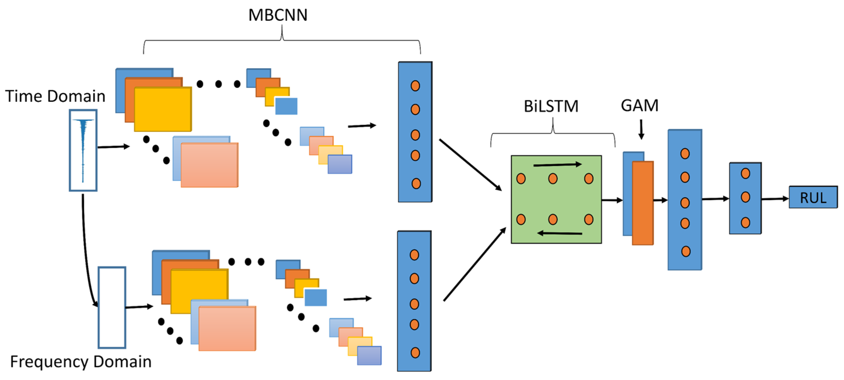
• A multi-branch convolutional neural network and a BiLSTM network are built for the extraction of bearing degradation features without traditional feature extraction.
• The advantages of the proposed method over other methods are verified on a publicly available bearing degradation dataset.

In this paper, the basic theory of CNN, BiLSTM and attention mechanism are introduced in Section 2. The algorithms and procedures of this paper are described in detail in Section 3. A publicly available bearing dataset is used in Section 4 to verify the feasibility and effectiveness of the method. Section 5 makes conclusions about this approach.

2. Theoretical Background

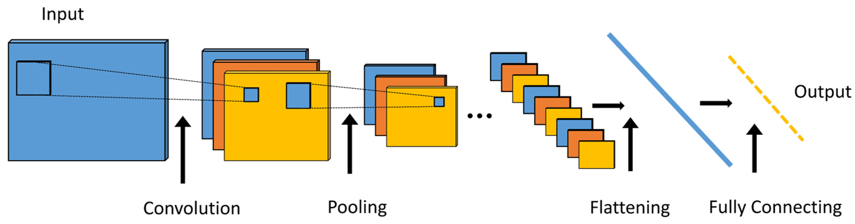
2.1. CNN Network

CNN is a representative feed-forward multilayer neural network [25] which has the role of feature extraction. The convolutional layer, pooling layer and fully connected layer are its main components. The convolutional layer performs convolutional operations on the input data, and the pooling layer performs dimensionality reduction on the input data. The convolutional layer and pooling layer work together to form a convolutional neural network, which performs layer-by-layer feature extraction on the input data and finally implements the regression or classification task by the fully connecting layer. The primary structure of CNN is displayed in Figure 1.

The core of a CNN is the convolutional layer. The convolution layer contains multiple convolution kernels, which convolve the input data using multiple specific weights. The convolution operation is a linear transformation that is implemented by locally weighting the input data. Since the vibration data of the bearing are one-dimensional data in this paper, we use one-dimensional convolution and the equation is shown below:

$$y_i=\sum _{n=1}^N{x}_n\ast w_{i,n}+b_i$$

(1)

where $x_n$ is the $n$-th partial input connected to the convolution kernel in the $i$-th channel; $N$ is the number of this input; $w_{i,n}$ is the weight of the $n$-th input part of the $i$-th channel; $\ast$ indicates the convolution operation; $b_i$ is the bias that in the $i$-th channel; $y_i$ represents the output that in the $i$-th channel.

Pooling is another important operation in CNN, by which the network output at a specific location is replaced with the summary statistics at a local location. Its main function is to raise the effectiveness of feature extraction and decrease the size of feature dimensions. From a certain point of view, it also plays a role in suppressing overfitting. Pooling mainly has maximum pooling and average pooling. Since the bearings’ degradation information is not obvious, where maximum pooling has the property of amplifying the information of finely differentiated features, maximum pooling is used in this paper. The calculation equation is illustrated below:

$$p^{l(i,j)}=\underset{\left(j-1\right)V+1\le t\le \mathit{jV}}{\max }\left\{a^{l(i,t)}\right\}$$

(2)

where $V$ denotes the range of the pooling; $a^{l(i,t)}$ is the activation value; $p^{l(i,j)}$ is the output after pooling.

Multi-branch neural network is a deep learning architecture based on CNN network, which contains multiple branches in the network, each with its own computational path. This architecture is able to learn and process multiple tasks simultaneously, thus increasing the efficiency and performance of the network. The bearings’ time domain information contains the vibration characteristics of the signal over time, and the frequency domain information contains the characteristics of the signal in terms of frequency, but does not contain the temporal time variation. So, only one domain or multiple domains combined for analysis cannot fully describe the degradation information of the bearing. Therefore, this paper uses a multi-branch branching structure with time and frequency domains as two branching inputs for bearings’ RUL prediction.

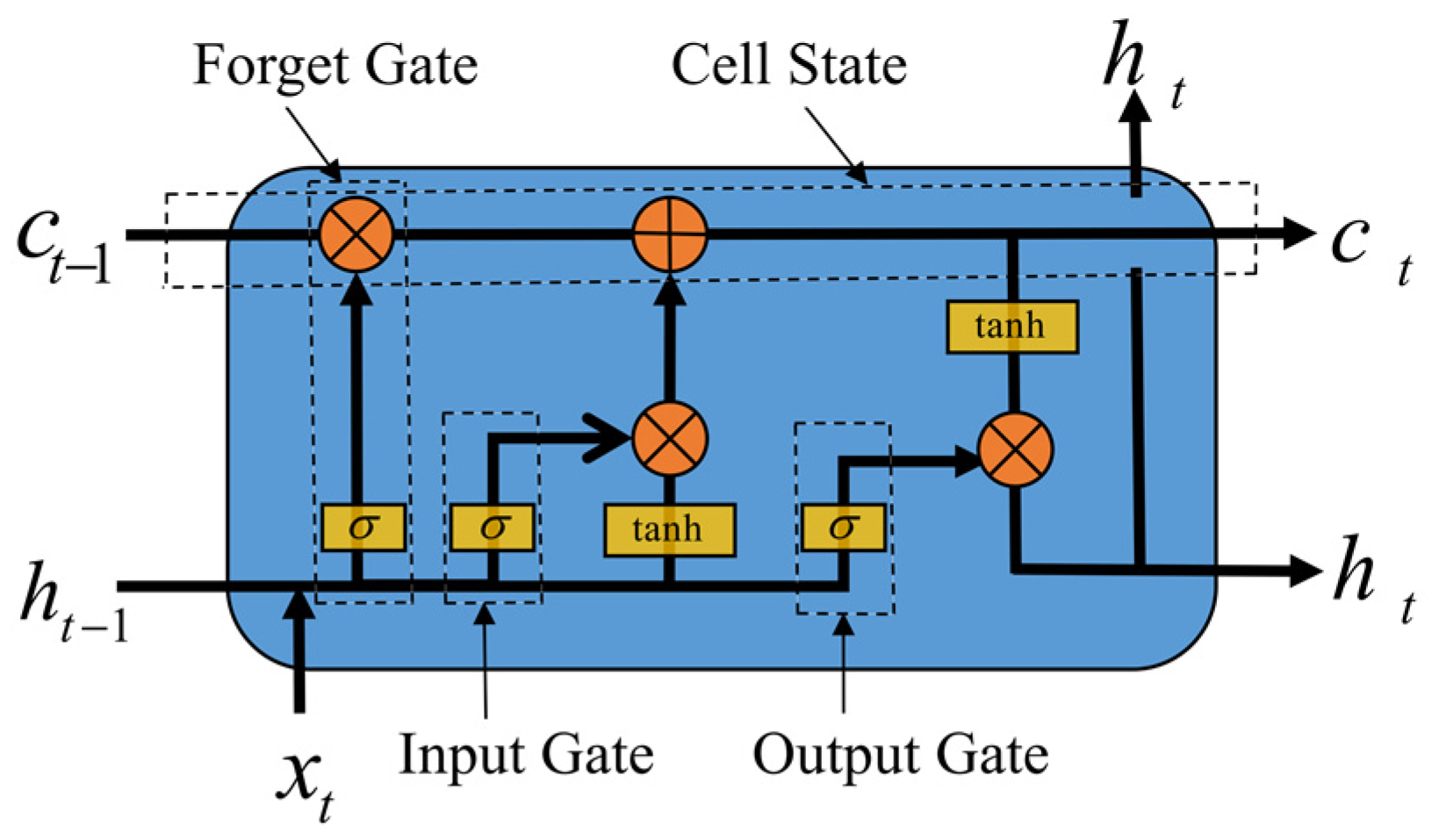
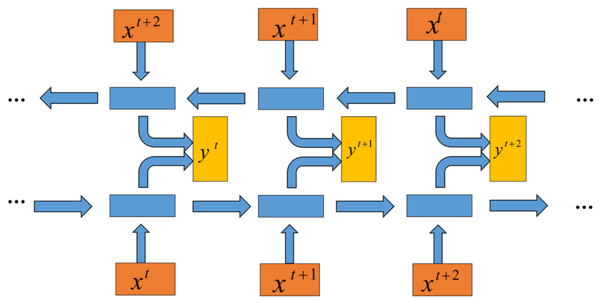
2.2. LSTM Network

The recurrent neural network (RNN) is specifically designed to deal with data related to time sequence, which can better deal with the temporally related problems by adding the relationship between front and back temporal order on the basis of fully connected neural networks. However, RNN networks have gradient disappearance and gradient explosion problems while processing long-term data and are not appropriate for long series forecasting. LSTM is a variant of RNN, which can better solve these problems, and its core lies in using cell states to record long-term historical information and manage it through various gate mechanisms. Its structure is illustrated in Figure 2. It mainly includes input gates, forgetting gates, cell states and output gates.

The Input Gate expressions are as follows:

$$Z^i=sigmoid(W_i·[V\left(W\left(i\right),h^{t-1}\right)]+b_i)$$

(3)

$$Z=tanh(W_c·[V\left(W\left(i\right),h^{t-1}\right)]+b_c)$$

(4)

The expression of the Forget Gate is as follows:

$$Z^f=sigmoid(W_f·[V\left(W\left(i\right),h^{t-1}\right)]+b_f)$$

(5)

The cellular update expressions are as follows:

$$C^t=Z^f\ast C^{t-1}+Z^i\ast Z$$

(6)

$$Z^o=sigmoid(W_o·[V\left(W\left(i\right),h^{t-1}\right)]+b_o)$$

(7)

The Output expressions are as follows:

$$h^t=Z^o\ast tanh\left(C^t\right)$$

(8)

where $W_i$, $W_f$, $W_c$, $W_o$ denote the weight matrix of the Input Gate, the weight matrix of the Forget Gate, the weight matrix of the current input cell state and the weight matrix of the Output Gate, respectively; $V$ denotes the merge operation on the matrix; $b_i$, $b_f$, $b_c$, $b_o$ denote the bias term of the Input Gate, the bias term of the Forget Gate, the bias term of the current input cell state and the bias term of the Output Gate, respectively; $Z^i$, $Z$, $Z^f$, $Z^o$ denote the Input Gate, the current input cell state, Forgetting Gate, and Output Gate, respectively.

Although the gradient disappearance and gradient explosion issues that arise in RNN can be mitigated in LSTM, its training of the network in prediction always propagates from front to back in the order of time series, with the result that it can only learn the information before the degradation of the current bearing and cannot fully utilize the information after the degradation of the current bearing. Since the current status of bearing degradation is relevant to the previous historical information, as well as being closely relevant to the subsequent information, this paper uses BiLSTM instead of LSTM for the temporal feature extraction of bearing degradation. The structure of the BiLSTM network is illustrated in Figure 3, which can fully exploit the bearing degradation time features and improve the data utilization and prediction accuracy.

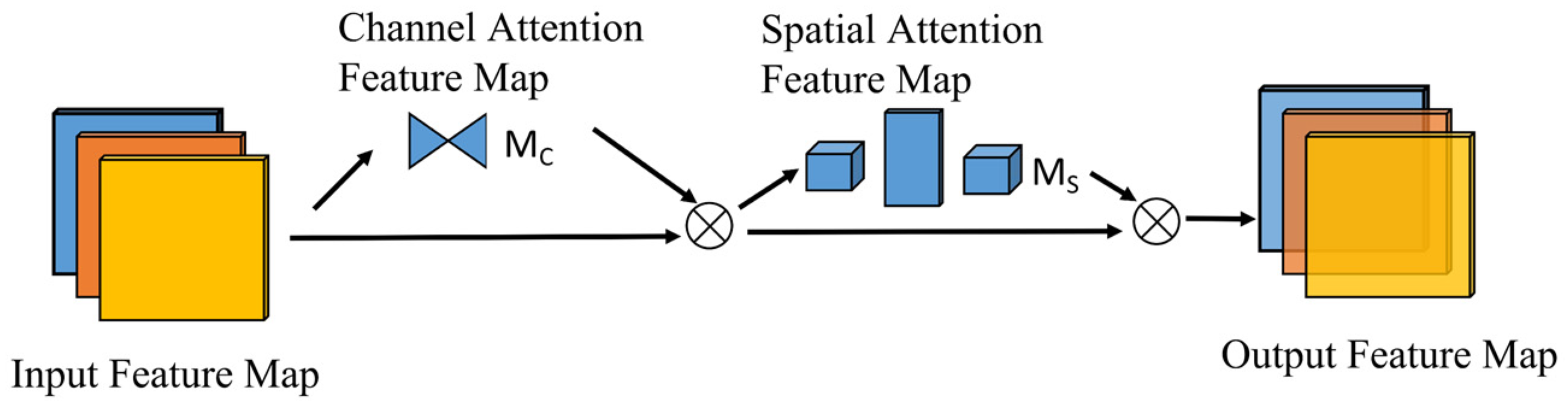
2.3. Attention Mechanism

Traditional neural networks cannot pay good attention to the degree mapped by different features in the feature extraction process. Adding attention mechanism to the network can focus on vital information and decrease the attention to redundant information, thus improving the accuracy and efficiency of feature extraction. In this paper, we use a global attention mechanism (GAM) which considers not only the channel information but also the cross-dimensional interaction information of channel information and spatial information [26]. It corrects the initial feature map by channel attention feature map (CA), and then corrects the correction result again by spatial attention feature map (SA) to obtain the final feature map. The GAM’s network structure displayed in Figure 4.

3. Proposed Method

Although the CNN network has a powerful spatial feature extraction capability, precisely because of its excellent feature learning capability, it may also tend to learn some useless information which is not conducive to the extraction of rolling bearing degradation features. On the other hand, although the BiLSTM network has strong temporal feature extraction ability, its spatial feature extraction ability is inferior to that of the CNN network. Therefore, this paper combines the two and uses a multi-branch approach. The main function of the MBCNN network is to extract spatial features and downsample the data, which plays the role of information refinement. The output is a feature map that is sparser than the original signal, but retains the spatial feature information of the data. The BiLSTM network extracts information that may be ignored by the CNN from both directions of the time series data. The structure of the MBCNN-BiLSTM model is illustrated in Figure 5. The original data and the frequency domain data obtained by fast Fourier transform are used as two branches of input to fully exploit the spatial and temporal feature information. An attention mechanism, GAM, is used to pay more attention to the important features in time and space. Finally, the RUL of the bearing is mapped by full connection to achieve the purpose of improving the accuracy of life prediction.

Figure 6 presents the flow chart of the proposed prognostic method.

The exact steps for the proposed approach to prediction are listed in the following:

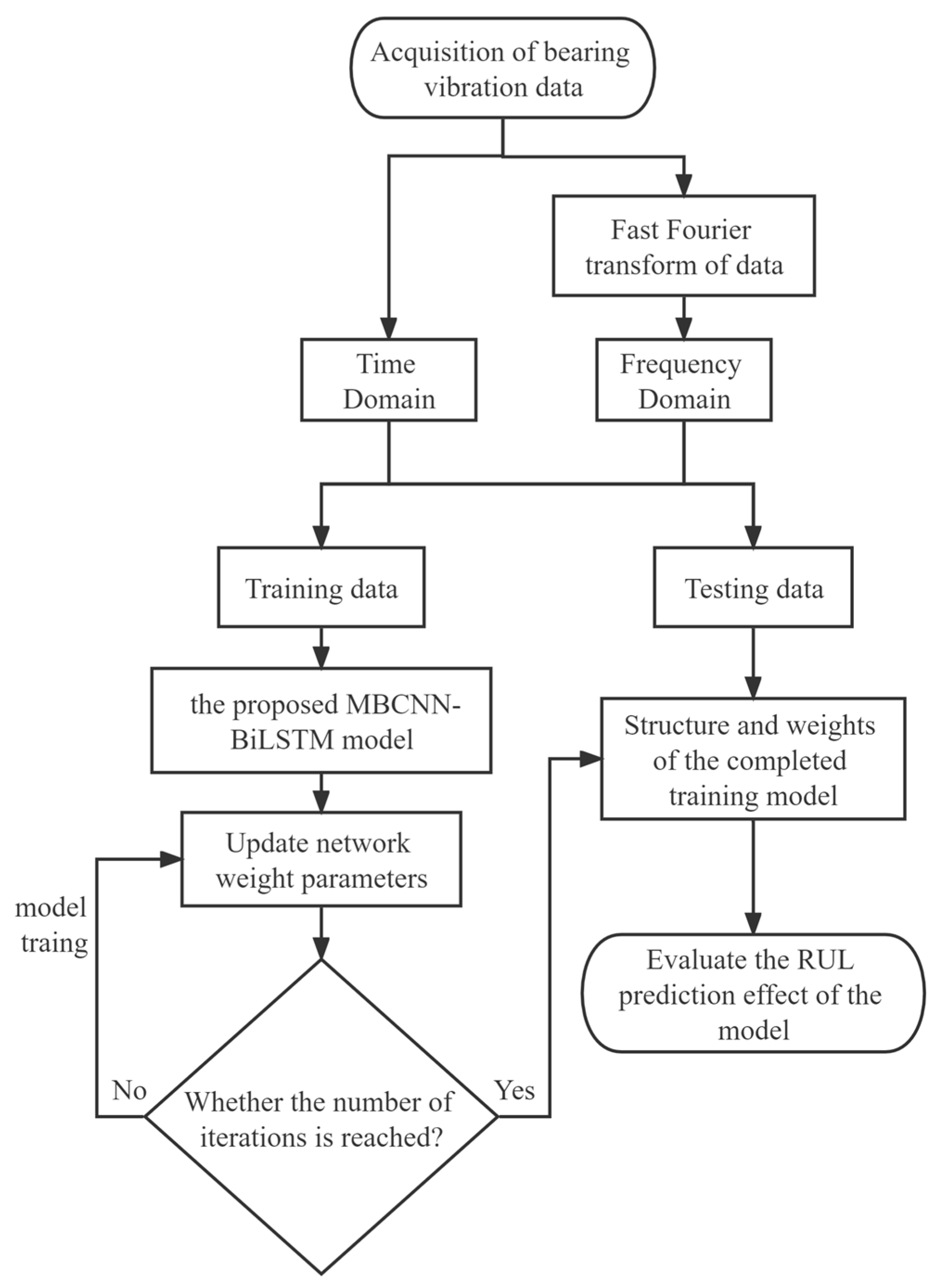
• Step 1. The fast Fourier transform is performed on the bearings’ originally vibrating signal to acquire the frequency domain signal, dividing the dataset into training set and test set based on the original signal and frequency domain signal. With the aim of improving the speed of training convergence of the network, the original vibration signal and the frequency domain signal are normalized. The data are preprocessed with the Z-Score normalization method. After normalization, the data exhibit a distribution with a mean of 1 and a standard deviation of 0. The equation is shown as follows:

  $$x_{norm}=\frac{x-\mu }{\delta }$$

  (9)

  where $x$ denotes the data sample; $\mu$ denotes the mean of the data sample; $\delta$ denotes the standard deviation of the data sample; $x_{norm}$ denotes the normalized data sample.
• Step 2. According to the RUL “end-to-end” prediction method, the bearing RUL labels are normalized and mapped to the range of 0–1, as follows:

  $$L_i=\frac{N-T_i}{N}$$

  (10)

  where $N$ denotes the total number of sampling points of the vibration signal for the whole life cycle of the bearing, that is, the actual RUL length of the bearing; $T_i$ is the $i$-th sampling point; $L_i$ is the bearing life label of the $i$-th sampling point. In this paper, the full-life degradation data of the bearing are mapped between 0 and 1. When the life label $L_i$ = 1 at the $i$-th time point, the bearing is a brand-new bearing. When $L_i$ = 0, the bearing has been completely damaged.
• Step 3. The data are divided according to the length of the set time window, and the data in each time window have a time order.
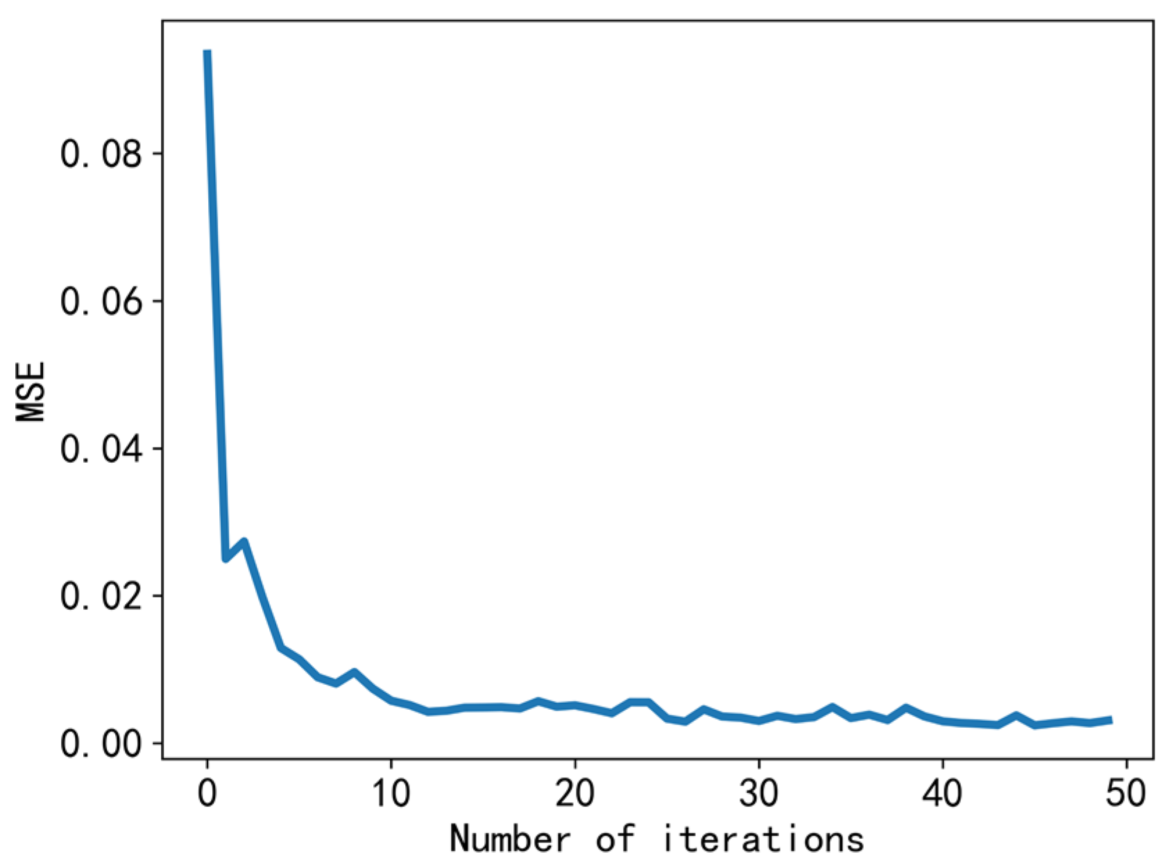
• Step 4. Model training. According to the MBCNN-BiLSTM model structure, the training hyperparameters are configured. The optimization algorithm of back propagation is used in the training period to optimize the network weights according to the loss function taking the minimum value, i.e., the minimum error of RUL between the true and the predicted.
• Step 5. Model evaluation. The data from the test set are input to the trained model to acquire the prediction results. The RUL prediction evaluation metrics are calculated according to the predicted and true values to get the RUL prediction performance of the model.

4. Experimental Study

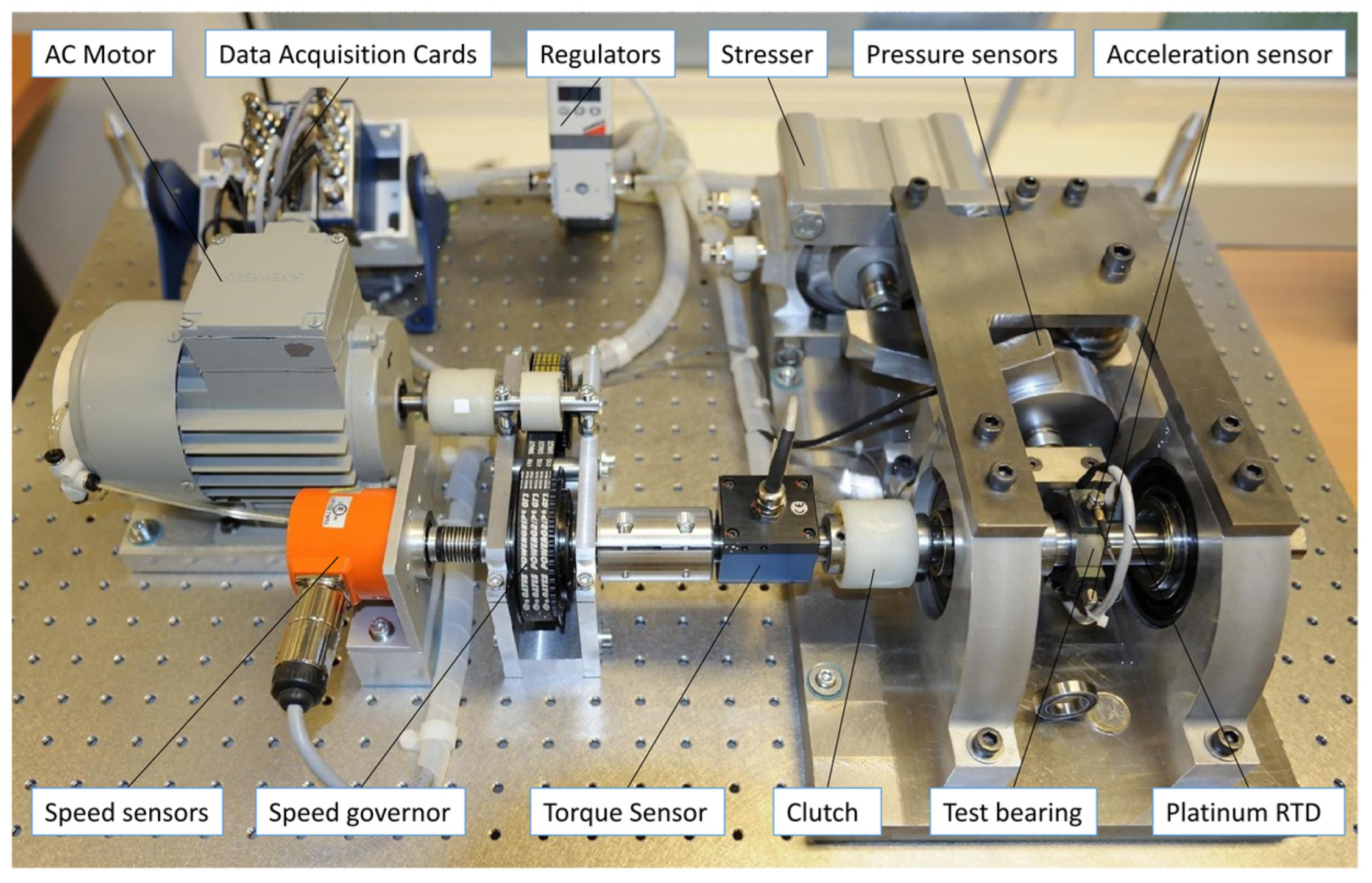
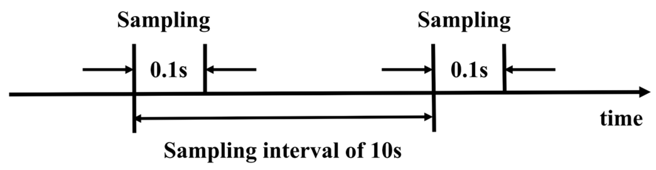
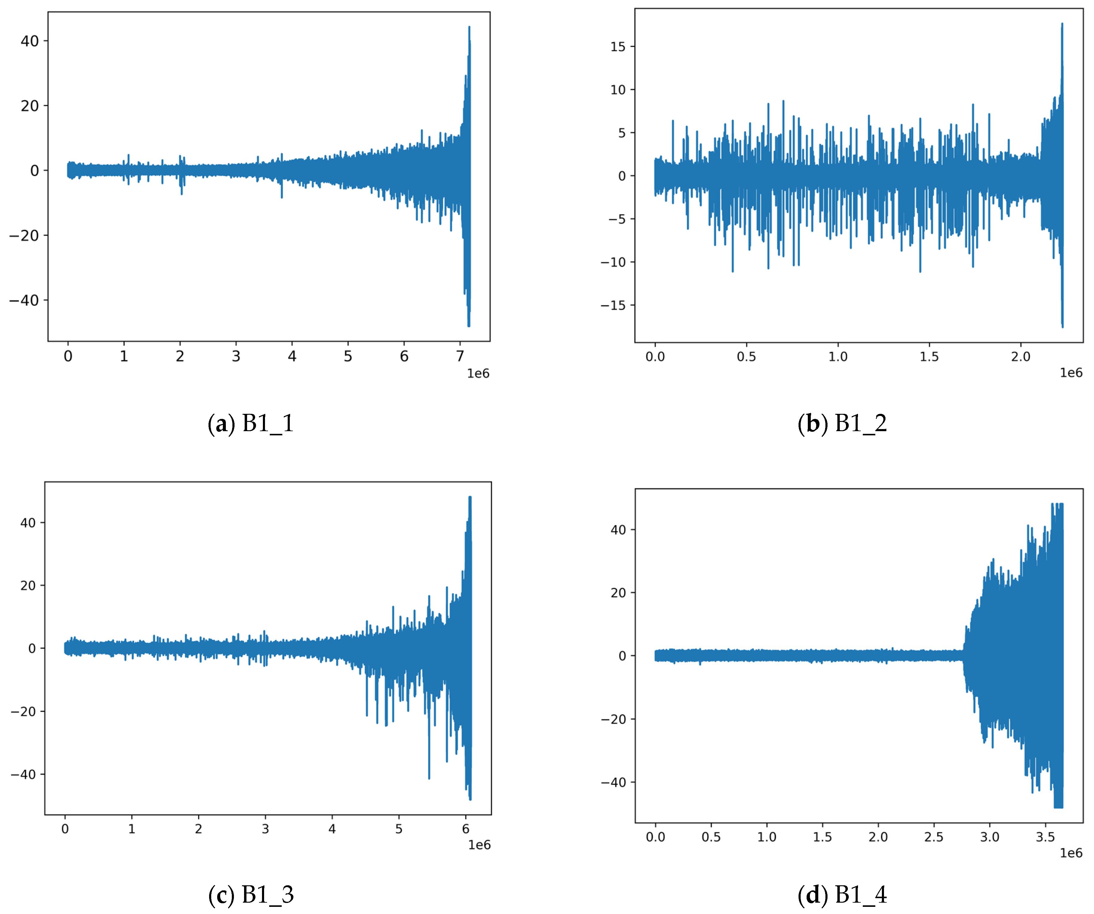
4.1. Experimental Data Presentation

With the aim of evaluating the effectiveness of the MBCNN-BiLSTM model introduced in this paper in RUL prediction, the accelerated degradation dataset of rolling bearings published in the IEEE 2012 PHM Data Challenge [27] in 2012 was used. This dataset was collected on the PRONOSTIA bearing accelerated degradation experimental platform, which is arranged as shown in Figure 7.

The wear is the main form of failure of rolling bearings, which generally occurs between the raceway and the rolling element. The wear will make the bearing clearance and surface roughness increase, and the rotational accuracy decrease, and will also intensify the bearing wear, which is mainly manifested as a vibration amplitude increase in vibration, so the fault diagnosis technology based on vibration signal has been widely used. Compared with signals such as temperature images, current and voltage signals, sound signals, and oil analysis, vibration signals respond quickly to changes in the state of the bearing, and contain the most useful information about changes in the operating state of the bearing; they are also easy to extract. Therefore, in this paper, the RUL of bearings is predicted based on vibration signals.

The experimental data were obtained by acquiring both horizontal and vertical acceleration sensors mounted on the bearing housing. The acquisition interval of the acceleration sensor is 10 s, the acquisition frequency is 25.6 kHz, and the time of each acquisition is 0.1 s, i.e., the number of data points acquired each time is 2560. If the vibration amplitude of the bearing vibration signal is more than 20 g, it is considered that the bearing is no longer usable. Its purpose is to prevent the destruction of the platform in the experiment while the amplitude of the bearing vibration signal is too large. The equipment collected vibration signals in both horizontal and vertical directions. It was studied that the horizontal signal provides more effective information than the vertical signal [28,29]; therefore, the horizontal signal was chosen for the experiments in this paper. The sampling schematic of this dataset is illustrated in Figure 8.

The dataset contains three operating conditions and a number of 17 bearings in total. The exact dataset description is illustrated in

Table 1. Description of the bearing dataset.

	Conditions 1	Conditions 2	Conditions 3
Radial force/N	4000	4200	5000
Rotational Speed/$\mathrm{r}·{\mathrm{m}\mathrm{i}\mathrm{n}}^{-1}$	1800	1650	1500
Bearing dataset	B1_1	B2_1	B3_1
	B1_2	B2_2	B3_2
	B1_3	B2_3	B3_3
	B1_4	B2_4	-
	B1_5	B2_5	-
	B1_6	B2_6	-
	B1_7	B2_7	-

.

Figure 9 shows the vibration waveforms in the horizontal direction of some bearings in operating condition 1. From the figure, it can be seen that as the bearings continue to degrade, their vibration amplitude becomes larger and larger, eventually leading to failure.

4.2. Experimental Parameter Setting

Based on the MBCNN-BiLSTM model, this paper designs the following parameters: a five-layer convolutional network, a one-layer BiLSTM network, a one-layer GAM network and two fully connected layers, and the last layer is the output layer. In addition, a BatchNormalization (BN) layer and a random deactivation (dropout) function are added to the network to prevent overfitting and enhance network robustness. Hyperparameters are used to define the structure of the neural network; however, there is no consensus on how to set these hyperparameters. This paper sets these based on the existing popular recommendations [18,21,23]. The detailed parameters of the model are provided in

Table 2. MBCNN-ABiLSTM model parameters.

Structure Name	Parameter	Activation Function
Convolutional layer 1	(16, 64, 16) (16, 64, 8)	ReLu
Convolutional layer 2	(16, 3, 1) (16, 3, 1)	ReLu
Convolutional layer 3	(32, 3, 1) (32, 3, 1)	ReLu
Convolutional layer 4	(64, 3, 1) (64, 3, 1)	ReLu
Convolutional layer 5	(64, 3, 1) (64, 3, 1)	ReLu
Fully connected layer 1	128	ReLu
Connect	-	-
BiLSTM layer	Hidden size 16	tanh
GAM layer	-	-
Fully connected layer 2	100	ReLu
Output layer	1	-

The table (16, 64, 16) indicates that a convolution kernel has a number of 16, a convolution kernel size of 64 and a step size of 16.

.

Since the bearing life prediction problem is a regression problem, MSE is chosen to be a loss function for model training; it is given by the following equation:

$$\mathrm{M}\mathrm{S}\mathrm{E}=\frac{1}{N}\sum _{i=1}^N{\left[f\left(i\right)-\widehat{f}\left(i\right)\right]}^2$$

(11)

where $N$ denotes the count of samples, $f\left(i\right)$ denotes the true RUL value that in the $i$-th sample, $\widehat{f}\left(i\right)$ denotes the prediction value of RUL that in the $i$-th sample.

For this paper, the model is trained for 50 rounds per experiment with a training batch size of 256. If the time window is too small, the prediction performance of the model is low. If the time window is too large, too much information is input to the model, which will increase the model training time. In order to maintain a balance between prediction performance and computational configuration, the time window size is set to 16. Since the Adam algorithm is currently the dominant neural network optimization algorithm, it is chosen for the network parameter optimization algorithm in this paper, and its initial learning rate is chosen to be 0.01. In addition, the computers for the experiments were configured as follows:

• The CPU is i9-10900H@3.7 GHz with 32 GB of memory;
• The GPU is NVIDIA Quadro P2200 with 5 GB of video memory;
• The operating system is Windows 10;
• The programming language is Python 3.10, which is implemented on the basis of the pytorch2.0 deep learning framework, and the experiments use the GPU to accelerate the speed of training.

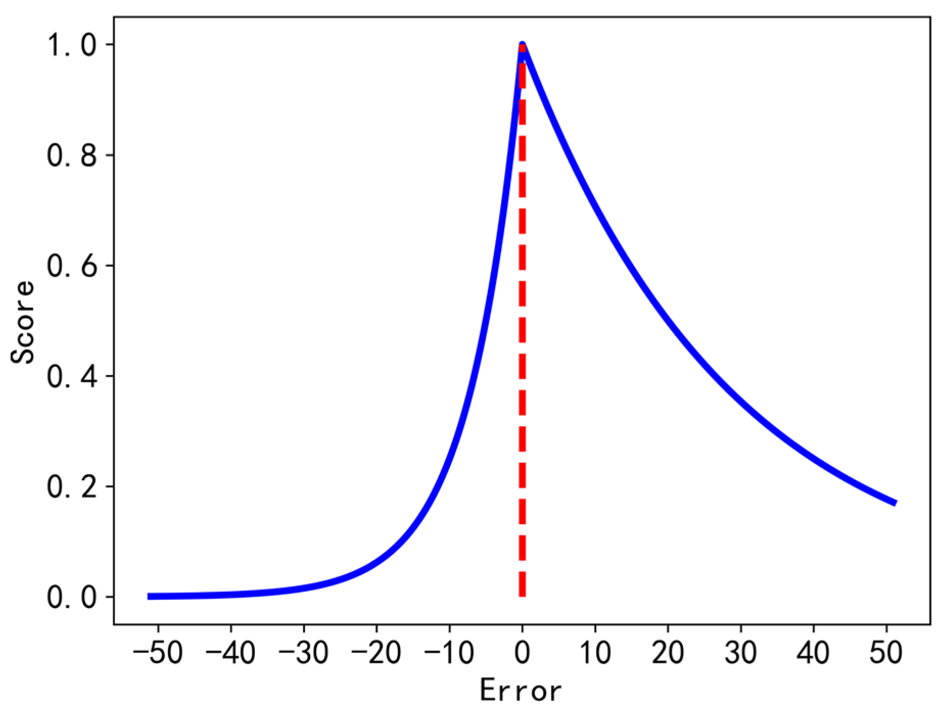
4.3. Performance Evaluation Metrics

The bearing life prediction problem is a regression problem in which the RUL of a bearing is the value of some continuous response variable. For better evaluation of the predictive effectiveness of rolling bearing RUL, mean absolute error (MAE), root mean squared error (RMSE) and scoring function are used as evaluation metrics to assess the effectiveness of the model; the formulas are as follows:

$$\mathrm{M}\mathrm{A}\mathrm{E}=\frac{1}{N}\sum _{i=1}^N\left|f\left(i\right)-\widehat{f}\left(i\right)\right|$$

(12)

$$\mathrm{R}\mathrm{M}\mathrm{S}\mathrm{E}=\sqrt{\frac{1}{N}\sum _{i=1}^N{\left[f\left(i\right)-\widehat{f}\left(i\right)\right]}^2}$$

(13)

$${Error}_i=\frac{{RUL}_i-\widehat{{RUL}_i}}{{RUL}_i}\left(100\%\right)$$

(14)

$$A_i=\left\{\begin{array}{c}{exp}^{-ln\left(0.5\right)·({Error}_i/5)}, {Error}_i\le 0\\ {exp}^{ln\left(0.5\right)·({Error}_i/20)}, {Error}_i>0\end{array}\right.$$

(15)

$$Score=\frac{1}{N}\sum _{i=1}^N{A}_i$$

(16)

where $N$ denotes the count of samples, $f\left(i\right)$ denotes the true RUL value in the $i$-th sample, $\widehat{f}\left(i\right)$ denotes the prediction value of RUL in the $i$-th sample, ${RUL}_i$ represents the true RUL value in the $i$-th sample, $\widehat{{RUL}_i}$ denotes the predicted RUL value in the $i$-th sample, ${Error}_i$ represents the RUL percentage error in the $i$-th sample.

The image of the functional relationship Score between and Error is illustrated in Figure 10. According to the graph, it is clear that the function values of positive and negative errors are asymmetric. The positive errors score higher than negative errors. In bearing RUL assessment, positive errors represent predicted RUL lower than actual RUL, i.e., life underestimation, and negative errors represent predicted RUL higher than actual RUL, i.e., life overestimation. The overestimation of bearing RUL will have risk, so life underestimation is more realistic than life overestimation.

4.4. Experimental Comparison Analysis

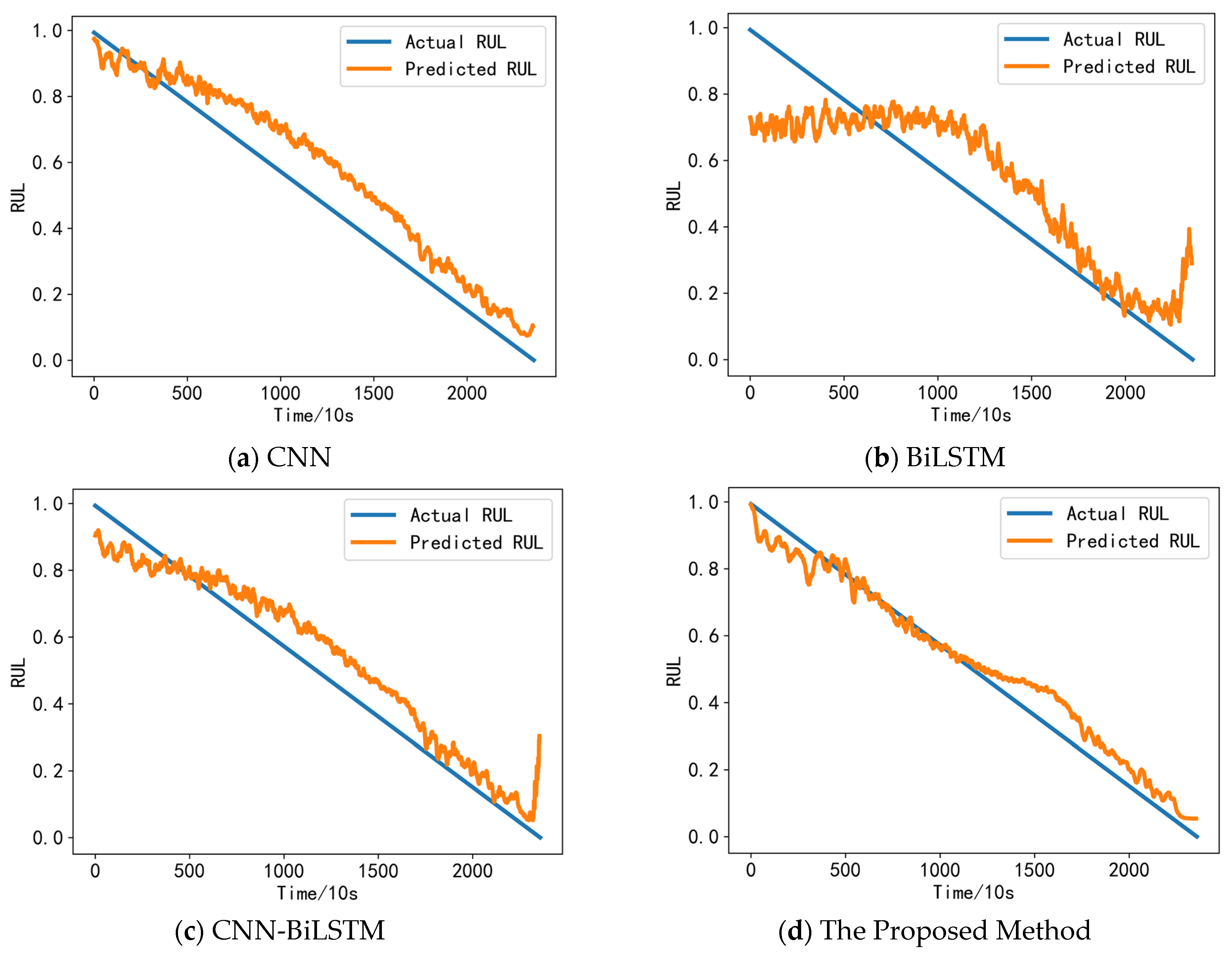
4.4.1. Experiments and Analysis of Different Models

For the purpose of verifying the effectiveness of the model suggested in this paper, B1_1, B1_2 and B1_4 of working condition 1 are selected as the training set and B1_3 as the test set. Meanwhile, three models are compared and analyzed with CNN, BiLSTM and CNN-BiLSTM. Figure 11 illustrates the change of the loss value of model introduced in this paper during training, which gradually decreases and eventually stabilizes as the number of training rounds increases. Figure 12 illustrates the RUL results for each model on the test bearings.

From Figure 12, the prediction curve of the CNN is clearly upward compared to the true curve, and there is a risk of overestimating the RUL of the bearing. The BiLSTM has the worst prediction effect. The model of CNN-BiLSTM has some improvement over CNN and BiLSTM. It is clear that the RUL prediction by the model of MBCNN-BiLSTM is closest to the real value.

To reflect on the model’s strengths and weaknesses more clearly, three evaluation indicators, MAE, RMSE and Score, are utilized in this paper to assess model’s performance. So as to prevent the effect of randomness of the experiments on the results, the average results of 20 experiments are used as the final results in this paper. The evaluation metrics of the prediction of each model are illustrated in

Table 3. Evaluation metrics values of the four models.

Model	MAE	RMSE	Score
CNN	0.09	0.10	0.43
BiLSTM	0.12	0.16	0.50
CNN-BiLSTM	0.07	0.08	0.51
MBCNN-BiLSTM	0.06	0.07	0.63

.

As evidenced by Table 3, the MAE, RMSE and Score of MBCN-BiLSTM outperformed the other three comparison models. Compared with CNN, BiLSTM and CNN-BiLSTM, the MAE values decreased by 33.3%, 50.0% and 14.3%, respectively, and the RMSE values decreased by 30.0%, 56.3% and 12.5%, respectively, and the scores improved by 46.5%, 26.0% and 23.5%, respectively, demonstrating the accuracy of the suggested model for bearing RUL prediction.

4.4.2. Experiments and Analysis with Different Existing Methods

For further validation that the proposed method in this paper is superior, it is compared with the method [15], method [23] and method [24], using B1_1 and B1_2 of working condition 1 as the training set and B1_3 and B1_4 as the test set. The results of the comparison of their MAE and RMSE values are illustrated in

Table 4. Evaluation metrics values of the four methods.

		Method [15]	Method [23]	Method [24]	The Propose Method
B1_3	MAE	0.14	0.12	0.09	0.07
	RMSE	0.31	0.16	0.12	0.08
B1_4	MAE	0.25	0.73	0.17	0.12
	RMSE	0.36	0.26	0.23	0.17

.

In test bearing B1_3, MAE values were reduced by 50.0%, 41.7% and 22.2%, respectively, and RMSE values were reduced by 74.2%, 50.0% and 33.3%, respectively. In test bearing B1_4, MAE values were reduced by 52.0%, 84.7% and 29.4%, respectively, and RMSE values were reduced by 52.8%, 34.6% and 26.1%, respectively. It fully illustrates the advantages of the suggested approach in this paper for the RUL prediction of bearing.

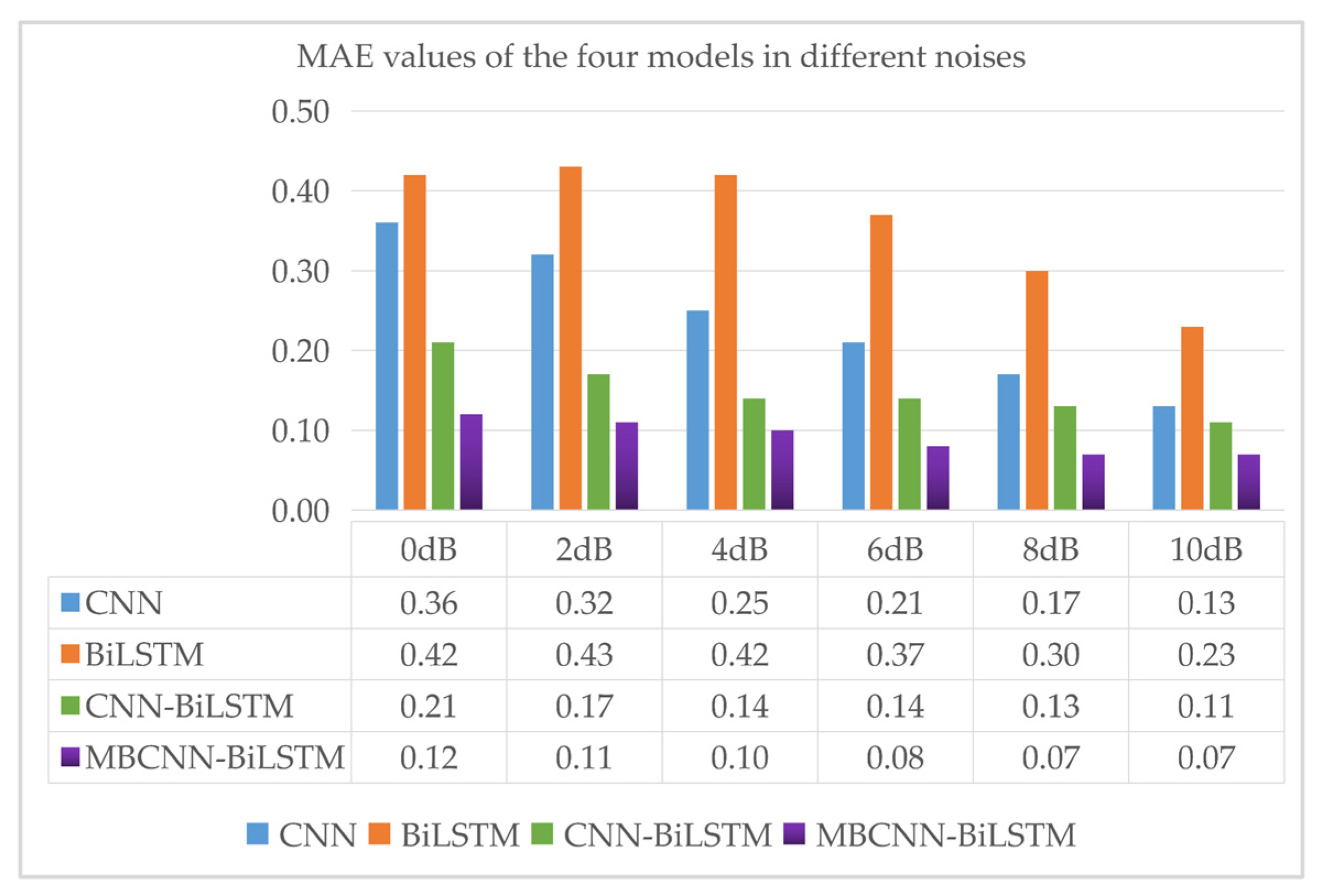
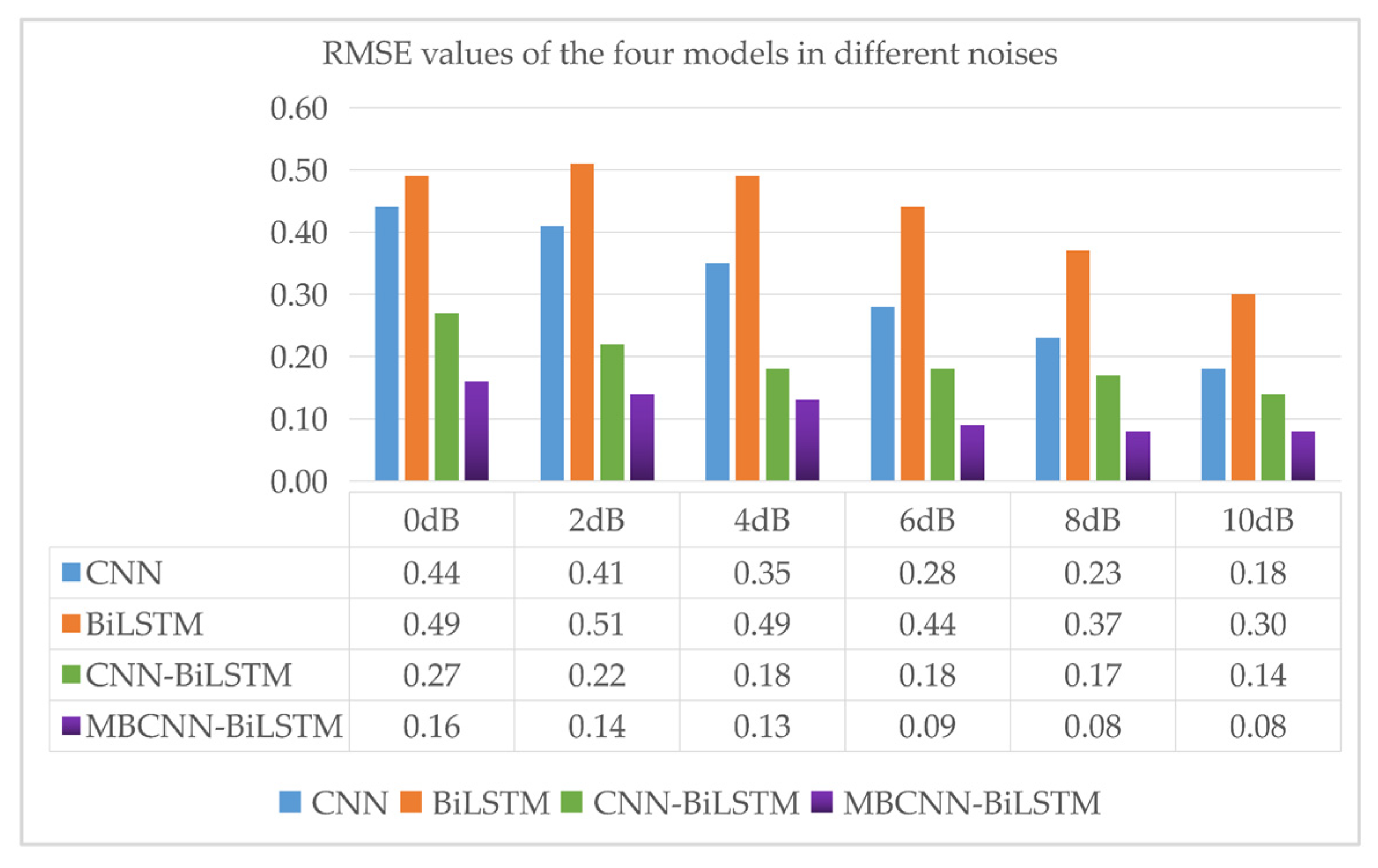
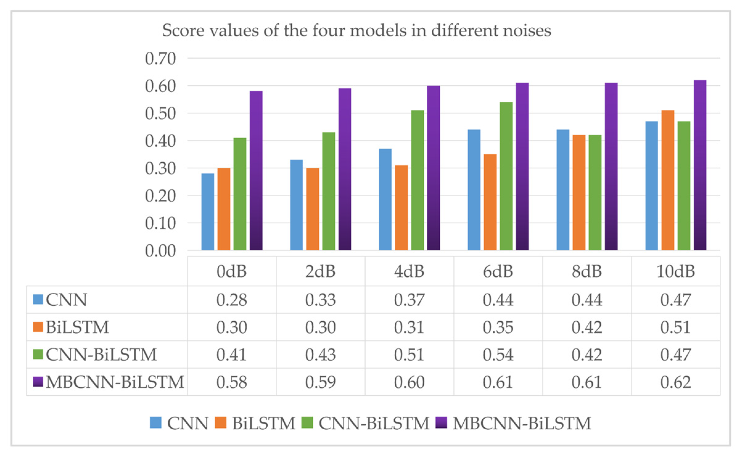
4.5. Noise Resistance Test

To explore the validity of the model to predict the RUL in a strong noise environment, B1_1, B1_2 and B1_4 of working condition 1 are selected as the training set and B1_3 as the test set. Meanwhile, three models are compared and analyzed with CNN, BiLSTM and CNN-BiLSTM. The model is trained using the training set, Gaussian white noise with different signal-to-noise ratios is added to the test set, the trained model is used to predict the RUL of the test set, and the signal-to-noise ratio is calculated as below:

$${SNR}_{dB}=10\mathrm{l}\mathrm{g}\left(\frac{P_s}{P_n}\right)$$

(17)

where $P_s$ is the effective power of the signal, and $P_n$ is the finite power of the noise.

In this paper, the test sets are constructed as 0 dB, 2 dB, 4 dB, 6 dB, 8 dB and 10 dB, respectively. The performance of MAE, RMSE and Score of each model in different noises are illustrated in Figure 13, Figure 14 and Figure 15, respectively.

As observed in Figure 13, Figure 14 and Figure 15, compared to other comparison models, the model proposed in this paper performs best in different noises and has stronger stability. The prediction accuracy of the model decreases with the increase of noise, but the model still has a high accuracy, which fully illustrates that the model can still make a more effective prediction of the RUL of the bearing in the face of the noise in the actual industrial environment.

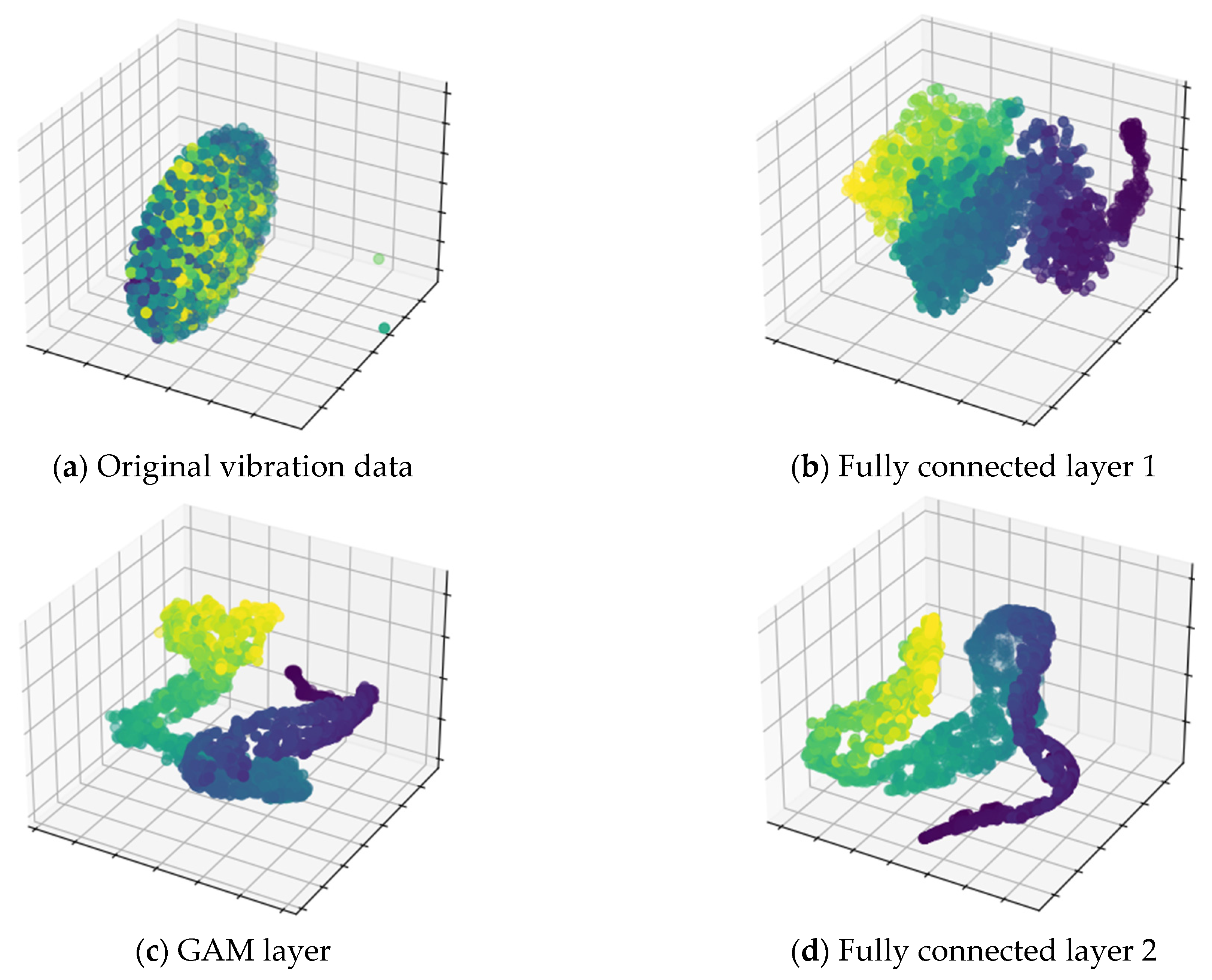
4.6. Visualization Analysis

To further analyze the feature extraction capability of the MBCNN-BiLSTM bearing RUL prediction model designed in this paper, the output of different hidden layers of the model was visualized and analyzed by dimensionality reduction using the t-SNE algorithm. Taking B1_3 as an example, the input layer, fully connected layer 1, GAM layer and fully connected layer 2 features were selected for visualization and analysis, and the results are displayed in Figure 16.

According to Figure 16, it is clear that the bearing degradation features are from disorder to order, which fully indicates that the proposed model has great feature extraction ability, and the bearing degradation trend can be better obtained by feature extraction of the final fully connected layer.

5. Conclusions

In this paper, a MBCNN-BiLSTM model is presented for the prediction of the RUL of bearings, and the effectiveness of the model is verified on the PHM2012 bearing degradation public dataset. The results of the study are as follows:

• The proposed method is an end-to-end bearing RUL prediction method, in which the original data are directly input into the network for RUL prediction without manual extraction of degradation features;
• The spatial feature extraction of the bearing input data is realized by MBCNN, and then BiLSTM further mines the data for temporal features. The GAM attentional mechanism is more conducive to focusing on the key information in the features, which improves the prediction accuracy of the bearings’ RUL;
• It has been shown that the average absolute error and root mean square error of prediction are reduced by “22.2%” to “50.0%” and “26.1%” to “52.8%”, respectively, compared with some existing prediction methods, which proves the effectiveness and feasibility of the proposed method. It is proved that the method proposed in this paper can reduce the prediction error in bearing RUL and has certain advantages over other methods.

The dataset used in this paper contains constant speed and constant load data, but the bearings in practical engineering applications usually operate under variable speed and variable load. In addition, we consider the RUL prediction of bearings for only one operating condition in this paper. One assumption of the deep learning approach used in this paper is that the predicted data need to follow a similar distribution as the historical data. However, the distribution is often different for different operating conditions and when the bearing data are dynamic. So, feature extraction becomes difficult to achieve in real industrial processes because the distribution changes. Transfer learning is a learning method in which similarities between tasks are used to apply knowledge gained in an old domain to a new domain. In future work, we will consider the application of transfer learning methods. In detail, sensor data from devices with different operating conditions or data from different devices can be used to achieve transferability of knowledge and thus improve the performance of RUL predictions.

References

- Singleton, R.K.; Strangas, E.G.; Aviyente, S. The Use of Bearing Currents and Vibrations in Lifetime Estimation of Bearings. IEEE Trans. Industr. Inform. 2017, 13, 1301–1309. [Google Scholar] [CrossRef]
- Safaeipour, H.; Forouzanfar, M.; Casavola, A. A survey and classification of incipient fault diagnosis approaches. J. Process Control 2021, 97, 1–16. [Google Scholar] [CrossRef]
- Tedesco, F.; Akram, W.; Forouzanfar, M.; Casavola, A.; Famularo, D. Predictive maintenance of actuators in linear systems: A receding horizon set-theoretic approach. Int. J. Robust Nonlinear Control 2022, 11, 6395–6411. [Google Scholar] [CrossRef]
- Islam, M.M.; Kim, J.M. Reliable multiple combined fault diagnosis of bearings using heterogeneous feature models and multiclass support vector Machines. Reliab. Eng. Syst. Saf. 2019, 184, 55–66. [Google Scholar] [CrossRef]
- Qin, Y.; Xiang, S.; Chai, Y.; Chen, H. Macroscopic-microscopic attention in LSTM networks based on fusion features for gear remaining life prediction. IEEE Trans. Ind. Electron. 2020, 67, 10865–10875. [Google Scholar] [CrossRef]
- An, D.; Kim, N.H.; Choi, J. Practical options for selecting data-driven or physics-based prognostics algorithms with reviews. Reliab. Eng. Syst. Saf. 2015, 133, 223–236. [Google Scholar] [CrossRef]
- Chen, C.; Li, B.; Guo, J.; Liu, Z.; Qi, B.; Hua, C. Bearing life prediction method based on the improved FIDES reliability model. Reliab. Eng. Syst. Saf. 2022, 227, 108746. [Google Scholar] [CrossRef]
- Cui, L.; Wang, X.; Wang, H.; Ma, J. Research on Remaining Useful Life Prediction of Rolling Element Bearings Based on Time-Varying Kalman Filter. IEEE Trans. Instrum. Meas. 2020, 69, 2858–2867. [Google Scholar] [CrossRef]
- Cui, L.; Wang, X.; Xu, Y.; Jiang, H.; Zhou, J. A novel Switching Unscented Kalman Filter method for remaining useful life prediction of rolling bearing. Measurement 2019, 135, 678–684. [Google Scholar] [CrossRef]
- Vashishtha, G.; Chauhan, S.; Yadav, N.; Kumar, A.; Kumar, R. A two-level adaptive chirp mode decomposition and tangent entropy in estimation of single-valued neutrosophic cross-entropy for detecting impeller defects in centrifugal pump. Appl. Acoust. 2022, 197, 108905. [Google Scholar] [CrossRef]
- Chauhan, S.; Singh, M.; Kumar Aggarwal, A. Bearing defect identification via evolutionary algorithm with adaptive wavelet mutation strategy. Measurement 2021, 179, 109445. [Google Scholar] [CrossRef]
- Chauhan, S.; Singh, M.; Kumar Aggarwal, A. An effective health indicator for bearing using corrected conditional entropy through diversity-driven multi-parent evolutionary algorithm. Struct. Health. Monit. 2021, 20, 2525–2539. [Google Scholar] [CrossRef]
- Ma, Q.; Lin, S.; Shen, L.; Wang, J.; Wei, J.; Yu, Z.; Cottrell, G.W. End-to-end incomplete time-series modeling from linear memory of latent variables. IEEE Trans. Cybern. 2020, 50, 4908–4920. [Google Scholar] [CrossRef]
- Chen, D.; Qin, Y.; Wang, Y.; Zhou, J. Health indicator construction by quadratic function-based deep convolutional auto-encoder and its application into bearing RUL prediction. Transactions 2021, 114, 44–56. [Google Scholar] [CrossRef]
- Loutas, T.H.; Roulias, D.; Georgoulas, G. Remaining useful life estimation in rolling bearings utilizing data-driven probabilistic E-support vectors regression. IEEE Trans. Rel. 2013, 62, 821–832. [Google Scholar] [CrossRef]
- Pan, Z.; Meng, Z.; Chen, Z.; Gao, W.; Shi, Y. A two-stage method based on extreme learning machine for predicting the remaining useful life of rolling-element bearings. Mech. Syst. Signal Process. 2020, 144, 106899. [Google Scholar] [CrossRef]
- García Nieto, P.J.; García-Gonzalo, E.; Sánchez Lasheras, F.; de Cos Juez, F.J. Hybrid PSO–SVM-based method for forecasting of the remaining useful life for aircraft engines and evaluation of its reliability. Reliab. Eng. Syst. Saf. 2015, 138, 219–231. [Google Scholar] [CrossRef]
- Han, T.; Pang, J.; Tan, A.C.C. Remaining useful life prediction of bearing based on stacked autoencoder and recurrent neural network. J. Manuf. Syst. 2021, 61, 576–591. [Google Scholar] [CrossRef]
- Qin, Y.; Chen, D.; Xiang, S.; Zhu, C. Gated dual attention unit neural networks for remaining useful life prediction of rolling bearings. IEEE Trans. Industr. Inform. 2020, 17, 6438–6447. [Google Scholar] [CrossRef]
- Wang, Y.; Ding, H.; Sun, X. Residual Life Prediction of Bearings Based on SENet-TCN and Transfer Learning. IEEE Access. 2022, 10, 123007–123019. [Google Scholar] [CrossRef]
- Jiang, C.; Liu, X.; Liu, Y.; Xie, M.; Liang, C.; Wang, Q. A Method for Predicting the Remaining Life of Rolling Bearings Based on Multi-Scale Feature Extraction and Attention Mechanism. Electronics 2022, 11, 3616. [Google Scholar] [CrossRef]
- Liu, Y.; Liu, Z.; Zuo, H.; Jiang, H.; Li, P.; Li, X. A DLSTM-Network-Based Approach for Mechanical Remaining Useful Life Prediction. Sensors 2022, 22, 5680. [Google Scholar] [CrossRef] [PubMed]
- Luo, J.; Zhang, X. Convolutional neural network based on attention mechanism and Bi-LSTM for bearing remaining life prediction. Appl. Intell. 2022, 52, 1076–1091. [Google Scholar] [CrossRef]
- Wang, X.; Qiao, D.; Han, K.; Chen, X.; He, Z. Research on Predicting Remain Useful Life of Rolling Bearing Based on Parallel Deep Residual Network. Appl. Sci. 2022, 12, 4299. [Google Scholar] [CrossRef]
- Rawat, W.; Wang, Z. Deep convolutional neural networks for image classification: A comprehensive review. Neural Comput. 2017, 29, 2352–2449. [Google Scholar] [CrossRef]
- Liu, Y.; Shao, Z.; Hoffmann, N. Global attention mechanism: Retain information to enhance channel-spatial interactions. arXiv 2021, arXiv:2112.05561. [Google Scholar]
- Nectoux, P.; Gouriveau, R.; Medjaher, K.; Ramasso, E.; Morello, B.; Zerhouni, N.; Varnier, C. PRONOSTIA: An experimental platform for bearings accelerated degradation tests. In Proceedings of the 2012 IEEE International Conference on Prognostics and Health Management, Denver, CO, USA, 18–21 June 2012. [Google Scholar]
- Soualhi, A.; Medjaher, K.; Zerhouni, N. Bearing Health Monitoring Based on Hilbert–Huang Transform, Support Vector Machine, and Regression. IEEE Trans. Instrum. Meas. 2015, 64, 52–62. [Google Scholar] [CrossRef]
- Singleton, R.K.; Strangas, E.G.; Aviyente, S. Extended Kalman Filtering for Remaining-Useful-Life Estimation of Bearings. IEEE Trans. Ind. Electron. 2015, 62, 1781–1790. [Google Scholar] [CrossRef]