1. Introduction
Machine learning not only influences the social media market but, simultaneously, it is highly capable of tracking the so-called unpredictable real-time matrices of growth, needs, results, and features. Machine learning is one of the most powerful tools to control the human mind′s transition through machine interpretation [
1,
2]. Individuals as well as sets of individuals using social media platforms are targeted by business media, multistoried companies, product sellers, and influencers. Facts and figures show that more than 56% of eighth-graders are additionally unhappy because their weekly social media involvement is over 10 h. Spending over 3 h per day on social media presents a high risk to the mental health of adolescents. According to the National Center for Health Research, 32% and 13% of children aged 12–17 suffer from depression and anxiety because of the inappropriate use of social media, respectively. Furthermore, 25% of 25-year-old adults have a mental illness, and they belong to the highest usage group [
3]. Apart from individual consumption, teenagers are experiencing crimes related to online harassment and cyberbullying. However, the numbers are only based on reported and known occurrences. Tracking particular algorithms behind the consumer attraction strategies of each social media platform is inconceivable and unrealistic [
4]. Still, in recent years, researchers have identified possible measurement factors to monitor the mental health of social media users using machine learning techniques [
5,
6]. Existing machine-learning-based solutions can predict a product value after studying historical sales-related data. For example, it can indicate the increase and decrease in the share market curve, and it can even measure the happiness index using behavioral analytics [
7,
8,
9].
1.1. Motivation
To analyze human emotion through a smart device or machine is challenging in reality. The method of measuring a person’s feelings using machine learning is known as sentiment analysis [
6]. There are several machine learning algorithms and classification models in development in data science for the application of the sentiment analysis method [
7,
8]. This subsection focuses on some of the relative research gaps and challenges we encountered in the field of sentiment analysis using machine learning approaches.
We found three fundamental difficulties in the sentiment analysis of an individual social media user, which are as follows:
A person is a user of different social media platforms;
Every social media platform offers diverse user access possibilities;
Different social media platforms have distinct emotional expression structures.
These three real-time complications lead to a lack of consistent interpretation among various social media accounts handled by a single person. Therefore, we incorporated social media accounts containing ontology with the help of data science to improve the sentiment analysis algorithm by making it more pertinent.
1.2. Contributions
Considering the survey reports and existing machine learning techniques, we propose an improved approach integrating the following features:
We propose an improved social media sentiment analytics technique through pleasure factor measuring to predict the individual state of mind of social media users and the ability of users to resist profound effects.
We suggest an integrated sentiment analysis machine learning model to compute the next best solution to a significant emotion value.
We consider dividing and seaming for two different but complementary estimation sentimental states, namely, happiness level counting and neutral expression level counting of each inter- and intra-linked expression.
We consider the integration of data through semantic-level interoperability from heterogeneous consequences.
With a high success rate, the proposed algorithm can track down more than one semantically linked activity from diverse social media platforms via a single user ID.
The rest of this paper is organized as follows: The related work section consists of existing research and describes the state-of-the-art in machine learning, sentiment analysis, information systems, and social media analytics.
Section 2 defines the problem statement behind our research goal.
Section 3 illustrates the proposed solution with algorithm selection and methodologies. Next,
Section 4 displays the outcomes of our proposed solution. Finally,
Section 5 concludes the paper with a description of the future aspects of the research area.
3. Proposed Solution
We intended to design an ML model to perform NLP, an improved social media sentiment analytics technique to predict the individual state of mind. The proposed estimation function tracks the counts of the aversion and satisfaction levels of each inter- and intra-linked expression through semantic level interoperability. It collects data from several social media posts, feedback, and reactions handled and expressed by a single user through the self-learning pipelining mode. Therefore, we aim to traverse peculiar sentiment reflections by a single user into different social media handles.
This section discusses how the pipeline of the proposed model helps to resolve existing difficulties. As shown in
Figure 1, the proposed ML model first semantically connects multiple (up to four) social media handles of a single person. Then, it collects data from semantically related classes into a single database. After that, the emotion score is counted for each input string with the help of an advanced NLP (natural language processing) strategy [
19,
20,
21,
22]. In this way, the model helps continuously monitor a person’s emotional outbursts from a neutral to a happy state and vice versa. The semantically interoperable property makes the model more competent [
23,
24,
25,
26]. It helps to analyze the overall activity of a person in their several social channels. It helps to estimate the satisfaction levels of each inter- and intra-linked expression.
The following steps to build such a model are shown in Algorithm 1. And the descriptions of each possible effort toward making this ontology are also defined in this section.
| Algorithm 1: Establishment of semantic level interoperability through ontology design. |
| Input: Data from different social media platforms of a person |
| Output: Semantically interoperable data |
| Initialization and declaration: |
| i. L1, L2: Linear expressions; |
| ii. T1, T2: Subjective terms; |
| iii. Y1, Y2: Variables; |
| iv. xsd: decimal, integer, long, short, byte; |
| v. ObjectProperty: OP |
| vi. InverseObjectProperty: IOP |
| vii. DataIntersectionOf: DIO |
| Start |
| Step 1: Entity selection: |
| (DataComparison(Arguments(Y1, Y2) comprel(Y1, Y2)))xsd |
| Step 2: Class identification: |
| i. ClassAxiom:= SubClassOf | EquivalentClasses | DisjointClasses | DisjointUnion |
| ii. ClassAssertion (DataHasValue (Y1 “R1”^^xsd:decimal) Y2) |
| iii. ClassAssertion(DataHasValue(Y1 “R2”^^xsd:decimal) Y2) |
| iv. EquivalentClasses(NormalSubstance DataAllValuesFrom(Y1 DataComparison(Arguments(T1 Y1) leq(T2 Y2)))) |
| Step 3: Object properties define: |
| i. IOP:= ′ObjectInverseOf′ ′(′OP′)′ |
| ii. ObjectPropertyExpression:= OP | IOP |
| iii. ′DataComparisonDefinition′ ′(′axiomAnnotations IRI DataRange′)′ |
| iv. ObjectAllValuesFrom: = ′ObjectAllValuesFrom′ ′(′OP/IOP ClassExpression′)′ |
| Step 4: Data properties define: |
| i. Variable: = NCName |
| ii. Rational: = Integer/NonZeroInteger |
| iii. Arguments: = ′Arguments′ ′(′NCName{NCName}′)′ |
| iv. DIO: = ′DIO ′(′DataRange DataRange{DataRange}′)′; DIO (xsd:nonNegativeInteger xsd:nonPositiveInteger) |
| Step 5: Annotation properties define: |
| i. Axiom: = Declaration | ClassAxiom | ObjectPropertyAxiom | DataPropertyAxiom | DatatypeDefinition | HasKey | |
| Assertion | AnnotationAxiom |
| ii. axiomAnnotations: = {Annotation} |
| *Annotation: ObjectIntersectionOf, ObjectUnionOf, ObjectComplementOf, ObjectOneOf, ObjectSomeValuesFrom, |
| ObjectAllValuesFrom, ObjectHasValue, ObjectHasSelf, ObjectMinCardinality, ObjectMaxCardinality, |
| ObjectExactCardinality, DataSomeValuesFrom, DataAllValuesFrom, DataHasValue, DataMinCardinality, |
| DataMaxCardinality, DataExactCardinality |
| Step 6: Individual definition establishment |
| i. ObjectHasValue: = ′ObjectHasValue′ ′(′ObjectPropertyExpression Individual′)′ |
| ii. ObjectHasSelf: = ′ObjectHasSelf′ ′(′ObjectPropertyExpression′)′ |
| iii. ObjectMinCardinality: = ′ObjectMinCardinality′ ′(′nonNegativeInteger ObjectPropertyExpression [ClassExpression]′)′ |
| iv. ObjectMaxCardinality: = ′ObjectMaxCardinality′ ′(′nonNegativeInteger ObjectPropertyExpression [ClassExpression]′)′ |
| Step 7: Define annotations; |
| Step 8: Ontology documentation: |
| ontologyDocument: = {prefixDeclaration} Ontology |
| prefixDeclaration: = ′Prefix′ ′(′prefixName ′=′ fullIRI′)′ |
| Ontology: = ′Ontology′ ′(′[ontologyIRI [versionIRI]] directlyImportsDocuments; ontologyAnnotations axioms ′)′ |
| ontologyIRI: = IRI |
| versionIRI: = IRI |
| directlyImportsDocuments: = {′Import′ ′(′IRI′)′} |
| ontologyAnnotations: = {Annotation} |
| axioms: = {Axiom} |
| End |
3.1. Semantic Interoperability
We choose web ontology language (OWL) [
25] to define possible semantic interoperability among the social media handlings by a single user id. It primarily helps to scale down the meaning of word expressions from comments, feedback, posts, and reactions on different social media platforms. It defines the equivalency and domain properties of distinct objects under similar classes. The consequence of the proposed ontology design has been described through Algo-rithm1, which carries the following steps:
3.1.1. Entity Selection
The entity selection defines the closure property of a set of declarations. Each IRI (internationalized resource identifier) utilized in an OWL entity is an axiom property that speaks about the class identification, object property, and datatype declaration. For the first-time entity declaration, it has to be defined which class data belong to whether they are individual or in combination. Most importantly, it enters the ontology vocabulary. The utilization of an existing entity could be possible simply by selecting or re-using it.
Declaration: = ′Declaration′ ′(′axiomAnnotations Entity′)′.
Entity: = ′Class′ ′(′Class′)′|′Datatype′ ′(′Datatype′)′|′ObjectProperty′ ′(′ObjectProperty′)′|′DataProperty′ ′(′DataProperty′)′|′AnnotationProperty′ ′(′AnnotationProperty′)′|′NamedIndividual′ ′(′NamedIndividual′)′.
3.1.2. Class Identification
Class and property construction could be complex as it represents a set of formal and individual special conditions. Instances of a particular class expression satisfy the requirements of a unique object property. ′ClassExpression′ represents class expressions in OWL, used to construct class identity. There are few inbuild or predefined class identifiers, like ′ObjectIntersectionOf′, ′ObjectUnion-Of′, ′ObjectComplementOf′, and ′ObjectOneOf′.
3.1.3. Object Properties Define
Object property expressions are a method to restrict the class expressions in the OWL platform. Some predefined object properties help express an object regionally. The ′ObjectSomeValuesFrom′ helps quantify an object property and holds at least one individual connection to the primary class property. In contrast, a universal quantification is conducted by the ′ObjectAllValuesFrom′ class expression. It joins the individuals linked via an object′s belongings countenance exclusively to instances of a disseminated class expression. An object property expression connects many distinct variables to a particular individual under the class expression ′ObjectHasValue.′ Ultimately, the ′ObjectHasSelf′ class declaration holds the individuals linked by an object property indication to themselves.
3.1.4. Data Properties Define
Restrictions on data property expressions help to define unique class expressions in OWL. Similar to limiting object property expressions, the leading contrast is that the existential and omnipresent quantification declarations permit n-ary data coverage. The ′DataSomeValuesFrom′ class declaration qualifies for a specified existential quantification from a checklist of facts-related expressions. It includes the individuals united via the data property countenances to the smallest literal within a given data field. There are two more data-restricted class expressions, like ′DataAllValuesFrom′ and ′DataHasValue.′ Data property cardinality restrictions also could be conducted using class expressions like ′DataExactCardinality′, ′DataMaxCardinality′, and ′DataMinCardi-nality′. Data types with range and domain are also specified during object property definition, like DataPropertyDomain: = ′DataPropertyDomain′ ′(′axi-omAnnotations DataPropertyExpression ClassExpression′)′, to explain the domain of a distinct data variable. Similarly, DataPropertyRange: = ′DataPropertyRange′ ′(′axiomAnnotations DataPropertyExpression DataRange′)′ declares the range of a certain variable.
3.1.5. Annotation Define
Applications of OWL frequently require tracks to associate supplementary knowledge with axioms, entities, and ontologies. Annotation defines this additional knowledge as axioms, entities, and ontology annotation. It is as simple as a general sentence that declares the domain and range of intercommunicated variables. However, the annotation syntax and structure of the comment and expression is defined by the ontology designer, independent of an ontology′s structural grammar.
3.1.6. Axiom
A bunch of hypotheses is the principal feature of an OWL ontology called axiom which looks like a statement that depicts the actual existence true to the domain. Axiom class in the structural specification in OWL is an extended comprehensive set of axioms. OWL axiom can be declarations about the classes, objects, or data properties. A class expression like class1 is a subclass of another class expression, such as class2, which could be expressed as a subclass axiom SubClassOf (class1 class2). Similarly, if a class expression like class1 is pairwise disjointed to class2, class3 and classn could be defined as:
DisjointClasses (Class1 … Classn). If a class, class1, is a disjoint union of the class declarations classi, 1 ≤ i ≤ n, it could be defined by the disjoint union axiom:
DisjointUnion (class1 … classn).
3.1.7. Individual Definition Establishment
In a domain, an individual represents the existence of an actual object through OWL syntax. Anonymous individuals and named individuals are two types of individuals in OWL syntax. Same objects are referred to in any ontology through an explicit name given by a named individual. In an OWL ontology, there are restrictions on identifying named individuals; reserved vocabulary cannot be used. However, anonymous individuals are regional to an ontology as they do not have a global name. In a resource description framework (RDF), anonymous or unidentified individuals are analogous to empty nodes. The representation of an individual is:
3.1.8. Ontology Documentation
A notional vision could be represented in phrases of structural specification using OWL ontology. An ontology document is associated with each ontology and physically stores the ontology in a specific way.
Free OWL tools offer OWL syntax that helps to store ontologies in a written text document format. The structural specification does not represent the ontology documents altogether. In contrast, OWL specification makes these two assumptions regarding their nature:
Every well-defined ontology converts into an ontology document that is a structural specification and illustrates the ontology UML class.
Using the appropriate protocol, an IRI helps to access individual ontology documents.
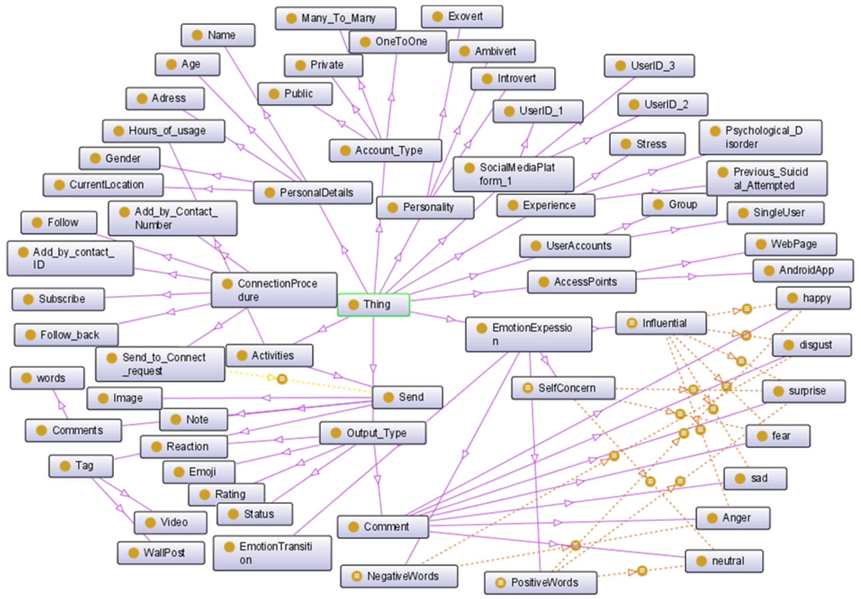
3.1.9. Semantic Interoperability Establishment
Semantic interoperability is not only concerned with the syntactical packaging of data but also the concurrent transmission of the semantics of those data (meaning). This procedure is performed by assessing metadata (data about the data) and merging the apiece data component into a shared and controlled vocabulary. Semantic interoperability makes a system understandable to an unknown system by taking the benefit of structural data exchange and vocabulary, including data codification. Therefore, the data interpretation becomes more accessible through information technology to the receiving end. The highest level of interoperability among the systems is represented by semantic interoperability. Semantic interoperability deals with the messaging format as well as concerns with the message content.
Figure 2 shows the resultant ontology graph view, for social media activity by single user ID, defined by OWL language.
3.2. Pre-Processing of the Text Data
In this phase, the machine learning process discovers pre-defined categories like abbreviations, unintentional characters, symbols, emoji, etc. Depending upon the use cases, there are several steps to pre-process the text data. We followed the sentiment classification standard by applying the natural language processing (NLP) model. Depending upon the subject of the consequence, we adopt seven sub-steps to pre-process our data, as follows in the following sections.
3.2.1. Remove Unconventional Space
Weird spaces can easily be removed from an input expression using a pre-defined natural language toolkit (NLTK) function in python. The operation removes unnecessary spaces from a sentence and returns join (text).
3.2.2. Tokenization
Tokenization of a sentence helps us reduce the number of words required to train a machine learning model. Tokenization not only converts words into tokens but also deals with the spaces into a phrase. From the NLTK library, we can refer to the ′word_tokenizer′ function or write our own. There are several tokenizer func-tions like ′word_tokenize,′ ′wordpunct_tokenize′, ′sent_tokenize′, etc. The ′word_tokenize′ function is based on treebank tokenizer, whereas the ′word-punct_tokenize′ function is based on simple regular expression.
3.2.3. Spelling Correction
The success of a real-time sentiment analyzer highly depends on the spelling correction phase. This particular level comprises two sub-layers: the embedding layer and bidirectional stacked char–long short-term memory (LSTM) network; it holds a collection of words or a language-based dictionary. Peter Norvig′s spelling correction method is highly preferred for social media data analysis among several spelling correction methods.
3.2.4. Contraction Mapping
The next crucial step is contraction mapping. A contraction is a squeeze or an abbreviated form of a succession of words. A computer considers a word and its contraction as two different expressions because it does not understand that contractions stand for abbreviations for a sequence of words and have a precisely similar meaning. As a result, it makes computation more expensive while raising the dimensionality of the composition span matrix by proffering two different columns. Contraction mapping replaces the abbreviation form with its valid syntax.
3.2.5. Stemming
Stemming is another essential step used in advanced machine learning procedures to reduce a word to its root form. Stemming and lemmatization are used alternatively in information systems because both the operations convert a term into its base form. But the fundamental difference between them is that lemmatization always reduces a word to a foundation form with linguistic meaning. In comparison, stemming may not be able to recede a word to its elemental composition with reasonable linguistic meaning. A different language is supported by distinct stemming or the lemmatization function in information systems. A linguistic specialist could develop a Lemmatizer, whereas we commonly use a stemming algorithm for data science purposes. NLTK supports several stemmers, like Porter stemmer, Snowball stemmer, Lancaster stemmer, etc. Ultimately, this sub-process reduces the training data volume needed to train our machine learning model.
3.2.6. Emoji Handling
Emoji handling is another essential step in pre-processing the data phase to analyze text data from multi-social media platforms. Here, we used a pre-defined emoji library to regulate the emoji.
3.2.7. Stop Words Handling
The final sub-step is to operate with stop words. This procedure helps to prioritize and filter out the words which could be considered as individual features in the case of NLP. In our case, the procedure also includes the cleaning of hypertext markup language (HTML).
3.3. Feature Extraction and Selection
Feature extraction and selection is a process to reduce data dimensionality. It helps to choose or select a more suitable input dataset (a subset of the available dataset) for a machine learning algorithm. If a feature set is defined by F(i) = {f1, …, fi, …, fn}, then the expected subset (F(s)) of selected features after this particular method could be expressed as F(s) F(i). However, this subset F(s) maximizes the learner′s proficiency by maximizing some mathematically defined scoring function. The feature selection mechanism fulfills two primary goals:
Dimensionality reduction occurs intending to encounter an optimal feature subset able to maximize the scoring function. In most cases, theoretically, Bayes error rate reduction is the best; however, often, the performance term is associated with the expectation by the chosen classifier model.
3.3.1. Bag of Words
Using a bag of words (BoW), a machine converts the word frequency matrix into its vector representation. The BoW document matrix could be of two types. One is BoW, and the other is binary BoW. For BoW, the machine is concerned with the frequency of a particular feature within each sequence. In binary BoW, the model is only concerned with the presence of the component in an input sequence. If a specific feature is present in the sequence, it is considered ′1′ or substituted by ′0′ if it is absent. The BoW procedure gives equal weightage to each present feature, providing poor semantic representation. We need another TF-IDF technique (term frequency and inverse document frequency) to solve this deficiency.
3.3.2. Part of Speech
Each word belongs to a general grammar category and is called a part of speech (PoS). Therefore, each order of a feature has its weightage towards the sentiment analysis of an input string.
3.3.3. TF-IDF and SVD
The most traditional way to handle text data has four pathways: hashing of words, count vectorization, term frequency–inverse document frequency (TF-IDF), and singular-value decomposition (SVD).
Likewise, in SVD, one can follow further steps: latent semantic analysis and scikit learn version of SVD for n numbers of components. It has already been verified that by applying TF-IDF and SVD together, a model can improve the result of logistic regression and XGB.
3.3.4. Word Embedding
A word-embedding layer is efficiently used in the practical implementation field of long short-term memory (LSTM), like sentiment analysis from text data. This layer is available in Keras. While coming to the word to vector (Word2Vec) feature extraction procedure, there are two-layered neural networks; they give a multi-dimensional word vector for every word in the dictionary or corpus a language has. Word2vec can represent a word or even a whole sentence in its vector form. It takes all the words in a sentence and tokenizes them, using only alpha-numeric words and removing the stop words. The process eventually appends everything to a list vector and normalizes it by the square root function of the sum over the columns.
3.4. Classification Model
We followed the proposed ML model, inspired by Algorithm 2, applying the advanced natural language processing (NLP) method. Depending upon the subject of the consequence, the steps of the algorithm are as follows in the next section.
3.4.1. Data Balancing
A deal imbalanced dataset is quite common in real-time classification problems. Sometimes the number of levels in one observation class is comparatively less than other target class levels. This kind of imbalanced dataset gives significantly inaccurate results in the classification method. There is a solution to this problem called resampling (oversampling and undersampling). The synthetic minority oversampling technique, or SMOTE, is an appropriate technique to oversample the minority class in our case.
3.4.2. Imputation
Imputation is a strategy that assists in retaining most of the data/information by substituting the missing data with alternate values in a dataset. Removing data is not feasible as it can lead to inappropriate size reduction, resulting in biasing and incorrect analysis by a model.
Most Python libraries do not have an inbuilt missing data handling strategy, and the ML model can lead to errors if the problem is not fixed. We can make an approach made up of several imputations for different classification model variables like numerical, date–time, categorical, and mixed (both for numerical and categorical) datasets.
| Algorithm 2: Proposed advanced NLP-based ML model. |
| Input: . |
| Output: Best fit solution for the proposed ML model. |
| Start |
| Step 1: Import libraries |
| Step 2: If count null from (): df.isnull().sum = 0; |
| Step 3: Calculate correlation: |
| where (= x and y variable sample, = means of values in x and y variables. |
| Step 4: Else |
| i. Remove null, replacing by most frequent occurrence; |
| ii. Repeat step 4; |
| Step 5: If () |
| Remove feature (: from (; |
| Step 6: Calculate feature importance: |
|
| where S: Unique class label numbers; : proportion between rows and output label. |
| Select top k features; |
| Step 7: Split train-test data sets; |
| Step 8: Best fit calculation: |
| i. ′n_estimators′: 1000, |
| ii. ′min_samples_split′: 2, |
| iii. ′min_samples_leaf′: 1, |
| iv. ′max_features′: ′sqrt′, |
| v. ′max_depth′: 25 |
| Step 9: rf_random.best_score calculation |
| Step 10: MAE, MSE, RMSE, R2 Score calculation |
| End |
3.4.3. Cross-Validation
Cross-validation is a technique in ML to test a model′s stability in terms of efficiency. Certifying an ML model is quite impossible, depending only upon the training dataset. Therefore, the cross-validation procedure first reserves a sample dataset from the primary dataset called the validation set; it is a subset of the initial dataset. Before deployment, an ML model is tested with this validation dataset, apart from the testing one. If the model performs well, then the model goes for the next step. This procedure checks the model′s efficiency by preparing the model with an input subset and testing the model on a prior unseen and independent input subset.
3.4.4. Hyper-Parameter Tuning
Some of the parameters in an ML model are predefined and not to be learned through training. These essential and fixed parameters, known as hyper-parameters, usually express several properties like the model′s speed or complexity.
4. Resultant Outcomes
The data from different social media platforms are diverse in type and length. Also, various expressions and actions define similar information. Because of this, a machine is uncertain about collecting each word′s emotional status and activity in an identical score bucket. We introduced a pipeline model able to include multiple hyper-parameters. Encountering the most satisfactory combination of such parameters is a searching procedure known as hyper-parameter tuning. GridSearchCV and RandomizedSearchCV are alternatively used for this hyper-parameter tuning process as demanded. First, we collected four datasets from four social media platforms with different patterns to design the model. We aimed to measure and analyze the interoperability value among those four social media platforms handled by a single user. Primarily the merged dataset includes the diverse level of emotion values for 1104 rows × 11 columns.
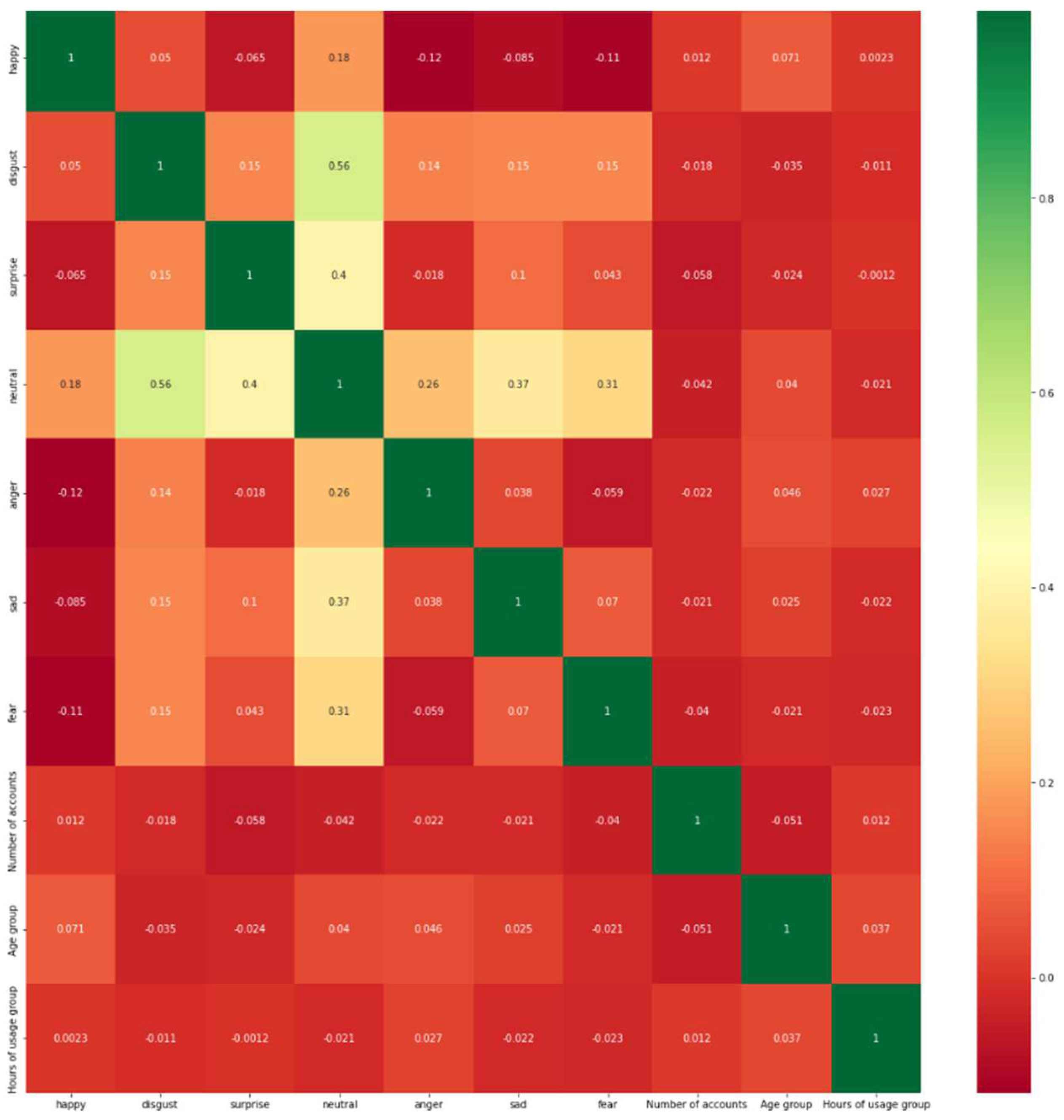
The dataset contains several numerical and categorical features like emotion values for a particular word, the number of accounts held by a single user, age group, hours of usage group, etc. As per the numerical computation, a specific word′s sentiment value is divided into essential parts like happiness, anger, disgust, surprise, neutral, sad, and fear. Apart from these, we considered up to four different accounts held by a single user id into four different social media applications. We also considered five diverse age groups of the users and up to 10 h of active usage. Next, we estimated the correlations among the features to choose the more effective variables, not the aggregate.
Figure 3 shows the heat map of the primarily considered features. We followed the Pearson’s Correlation coefficients as the correlation measurement function.
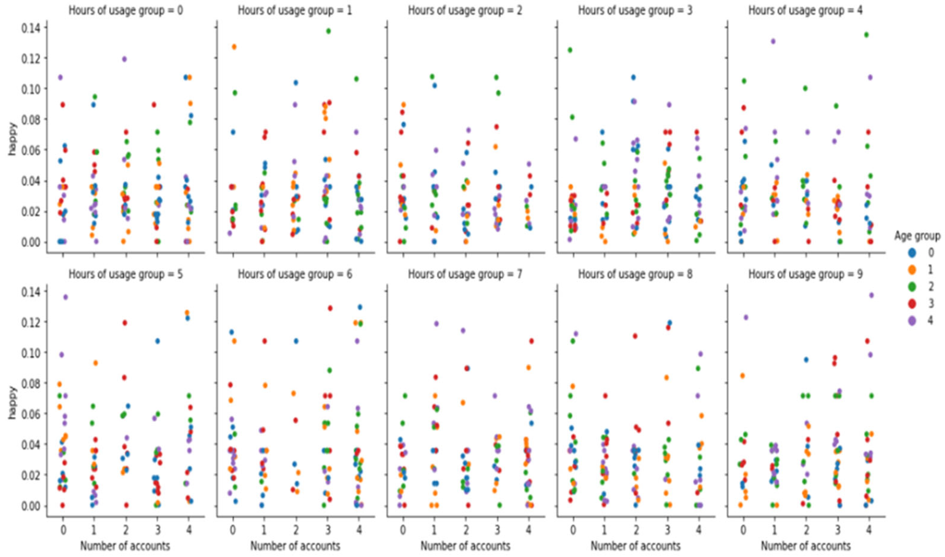
Like line graphs, two-dimensional scatter plots show the impact of one variable upon another with the help of dots against horizontal and vertical axes. We observed data visualization by ′multivariate′ or ′multi-variable′ scatter plot visualization. Precisely, the relationships between numerous dataset attributes are comprehended by multivariate visualization.
Figure 4 depicts the relation between happiness values concerning total hour-wise activity on a number of social media accounts.
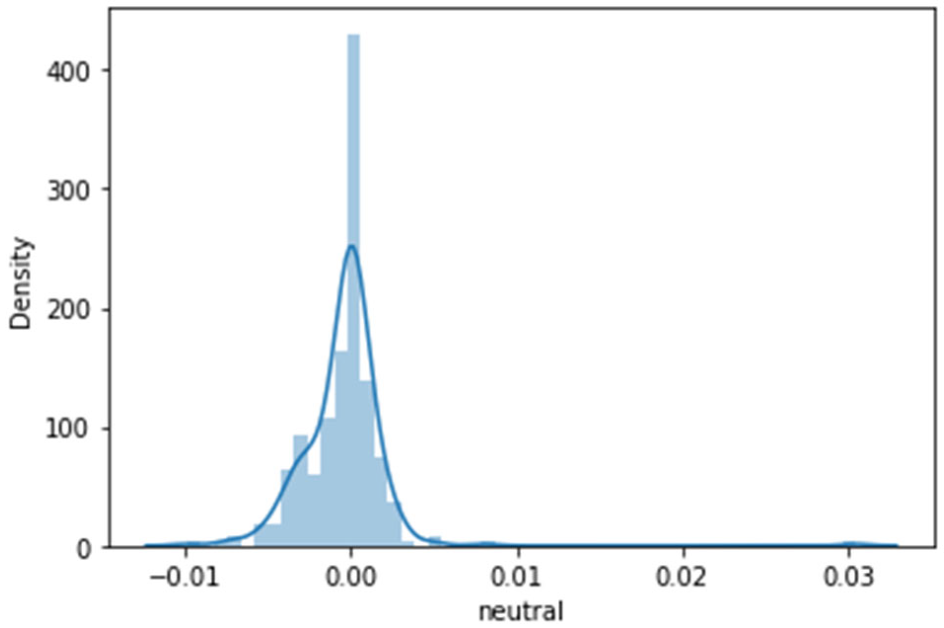
A density plot is another straightforward and convenient approach for obtaining each distributed attribute in one frame. Density plotting is most likely a histogram, connecting each domain′s top by a smooth curve, also known as abstracted histograms.
Figure 5 is the plotted density plot concerning happiness significance. The range (with α value 0.12) and domain of the curve are significantly satisfactory.
We decided to choose the random forest regressor to split the dataset into train and test sub-datasets. And, in the case of the tuning of hyper-parameters, we set randomized search CV. We selected the random forest regressor function in our case as we have mixed dataset features (both numerical and categorical). This particular regression provides limited explaining ability with a high prediction accuracy for integrated datasets.
Primarily, we experimented with two ways to train our model: one considering all primary features and the other after discarding the features based on the correlation factor.
Figure 6 shows the correlation heat map among the effectively correlated features. Furthermore, we continued with the effectiveness calculation after pitching the less convincing variables.
From the learning algorithm′s perspective, the relevancy of a feature could be defined in many ways. It may intend to determine the relevance of a particular feature; it could be the overall relevancy among all the features. Two degrees of significance are mostly counted when the machine searches for strong and weak relevance. A distinct feature is trusted as relevant if it has a strong or weak relevance score; otherwise, it is discarded from the dataset. An optimal Bayes classifier determines the strong relevance of a feature or variable in such a way that the resultant performance of the overall ML model could be deteriorated depending upon one variable/feature vi.
Where the set of features/variables Fi = {v1, …, vi − 1, vi + 1, … vn}, except vi. vi is considered a strongly relevant feature if p(vi = xi, Fi = fi) > 0 for some existence of xi, y, and fi. A value-assignment fi denotes over each feature from Fi, such that:
p(
Y = y |
vi =
xi;
Fi =
fi) ≠
p(
Y = y |
Fi =
fi)
. p stands for the performance variable of an optimal Bayes classifier.
Figure 7 shows the relevancies of different features during model training.
Similar to the previous case, we followed the random forest regressor [
27] to split the dataset into train and test sub-datasets. And, in the case of hyper-parameters tuning, we set randomized search CV. Concerning the neutral emotion values, the density curve shows how much the range is relatively less than in the last case. The confidence region has reduced significantly as the arc is sharper in shape, and the alpha value is now 0.02, which is pretty much effective in the case of emotion detection.
Figure 8 is the ultimate density curve for our improved ML model concerning the most stable emotional state, i.e., the neutral state.
Figure 9 shows the scatter plot of the test dataset after the model′s training with best-parameter tuning and selection. Furthermore, MAE, MSE, RMSE, and R2 values [
28] have evaluated the measures of the ultimate model performance [
3], shown in
Table 1. All the measurements support the success of our proposed model. Like the R2 value assured, 97% of the model′s inputs can explain the observed variation, which is favorable and satisfactory.
Semantic level interoperability through defined ontology has made it possible to collect data from distinct social media platforms; hence, we have integrated and illustrated training datasets. The model has been further improved compared to the previous case of feature selection. Consequently, we enhanced the proposed model′s efficiency by selecting effective features from the collected dataset.

 ,
, 


