Determination of Hydrogen’s Thermophysical Properties Using a Statistical Thermodynamic Method

Abstract

Accurate determination of the thermophysical properties of hydrogen is a crucial issue in hydrogen system design. By developing computational programs, a statistical thermodynamic model based on fundamental equations of state was implemented to determine hydrogen’s thermophysical properties, including the ortho-hydrogen fraction in equilibrium hydrogen, para-ortho hydrogen conversion heat, isobaric heat capacities and enthalpies. The deviations of calculated para-hydrogen enthalpies from REFPROP data were within 2.22%, ranging from 20 K to 300 K at 0.1 MPa, and within 2.32% between 100 K and 1500 K at pressures from 0.1 MPa to 20 MPa. To quantitatively assess the convenience of the statistical thermodynamic method, the running speeds of programs with different methods for determining hydrogen’s thermophysical properties were compared. The time required for statistical thermodynamic calculation was 7.95% that required for treading REFPROP data when the performance of the variable density multilayer insulation combined with a one vapor-cooled shield and para-ortho hydrogen conversion was calculated. The programs developed based on the statistical thermodynamic method can be used to determine the thermophysical properties of hydrogen or other fluids.

1. Introduction

Hydrogen (H₂) is widely used in the production of chemicals [1], petroleum refining [1], fuel cells [2], internal combustion engines [3] and aerospace engineering as rocket fuel [1]. Hydrogen has two spin isomers: ortho-hydrogen (ortho-H₂) and para-hydrogen (para-H₂), which have different rotational states. The equilibrium mixture ratio of the two forms changes with temperature [4]. They have considerably different rotational energies below 250 K. Their caloric properties, such as isobaric and isochoric heat capacity, thermal conductivity, enthalpy and entropy show significant differences [5]. Thus, accurate determination of hydrogen’s properties is essential for product and process designs in hydrogen industries [6,7], like hydrogen liquefaction and cooling capacity utilization.

Equations of state (EOSs) for hydrogen are the basis for determining the thermophysical properties of hydrogen. Redlich and Kwong [8] developed the Redlich–Kwong state equation of actual gas based on the van der Waals equation. Goodwin [9] derived the second and third virial coefficients for para-H₂ from experimental P-V-T (pressure–volume–density) data [10]. Goodwin [11] developed a new EOS for para-H₂, which employed one set of 24 coefficients for all fluid states. McCarty and Weber [12] established a 16-term polynomial EOS for para-H₂ up to 2778 K and 69 MPa [7]. McCarty [13] proposed a 32-term modified Benedict–Webb–Rubin (MBWR) EOS for para-H₂ from the triple point to 2500 K at pressures up to 68.9 MPa (680 atm). In 1982, Younglove [14] developed models based on the MBWR equation to determine the thermophysical properties of para-H₂ and other fluids, such as argon, ethylene and nitrogen. These models were used in previous versions of the NIST (National Institute of Standards and Technology) standard property package, REFPROP (Reference Fluid Thermodynamic and Transport Properties Database). Jacobsen [15,16] proposed an EOS explicit in the Helmholtz free energy, and extended the applicability of the Helmholtz-type EOS to 15 cryogenic fluids, including normal hydrogen. All thermophysical properties (compressibility factor, internal energy, enthalpy, entropy, speed of sound and isobaric/isochoric heat capacity) are derived via the differentiation of the Helmholtz free energy. Kunz [17,18] developed Helmholtz-type equations (GERG-2004 and GERG-2008) of natural gas (21 components) by combining them with the EOS for pure fluids. GERG-2008 covers the gas phase, liquid phase, supercritical region and vapor–liquid equilibrium states, with a range of validity of 60–700 K and up to 70 MPa. Leachman [5,19] created three new 14-term fundamental EOSs for para-H₂, ortho-H₂ and normal H₂. They are explicit in the reduced Helmholtz free energy. Despite the absence of the experimental data of normal H₂ and ortho-H₂, the quantum law of corresponding states was applied to improve their formulations. Consequently, thermophysical properties near the critical point and in liquid states can be accurately determined. The aforementioned three EOSs can be applied at pressures up to 2000 MPa and temperatures up to 1000 K.

Early EOSs for hydrogen explicit in pressure are sometimes unavailable near two-phase or supercritical regions. Thermodynamic properties, such as entropy, enthalpy and isobaric heat capacity (c_p), are derived from integrals of pressure or density. The continuity of an EOS has a great impact on the feasibility of integrals, and causes difficulties or instability in computation. However, all thermodynamic properties can be obtained via the differentiation of Helmholtz free energy from the fundamental EOS. In addition, ortho-H₂ properties should be considered in the design of processes, including para-ortho H₂ conversion. Hence, Leachman’s [5,19] equations were selected for this study because they cover the EOS of ortho-H₂. The thermophysical properties of hydrogen can be determined by taking at most second-order derivatives of the Helmholtz free energy with respect to temperature or density based on the fundamental EOSs.

Reading data from RREPROP is another typical method used to determine the thermophysical properties of hydrogen. Sometimes, the thermophysical property data in RREPROP are listed in a database for a finite number of states. In a limited range, spline interpolation is used to predict properties in arbitrary states.

In this study, the thermophysical properties of hydrogen were obtained by developing computational programs based on the statistical thermodynamic model. The ortho-H₂ fraction in equilibrium hydrogen (equilibrium H₂) and the para-ortho H₂ conversion heat were derived from the nuclear rotation partition functions of ortho-H₂ and para-H₂. The isobaric heat capacity and enthalpy were derived from Leachman’s [5,19] fundamental EOSs. To compare different methods for determining hydrogen’s thermophysical properties under an engineering background, a vapor-cooled shield (VCS)—a multilayer insulation (MLI) combined structure for liquid hydrogen storage—was investigated. The heat transfer model for the VCS-MLI was introduced and validated. The thermophysical properties were obtained via different methods, and the accuracy of the statistical thermodynamic method was verified using REFPROP data and other researchers’ results. Then, three tests were conducted to quantitatively analyze the convenience of the statistical thermodynamic method by comparing the running speeds of programs with different methods. These methods include statistical thermodynamic calculation, reading REFPROP data, spline interpolation, etc. When the performance of a VCS-MLI structure integrated with para-ortho H₂ conversion was predicted, the statistical thermodynamic method can save about 92% of the time consumed by reading REFPROP data. The developed programs based on the statistical thermodynamic method can also be applied to determine the thermophysical properties of other fluids.

2. Theoretical Model and Implementation

2.1. Statistical Thermodynamic Model for Hydrogen

Statistical thermodynamics is a basic tool used to obtain thermophysical properties theoretically. Equilibrium H₂ is composed of specific proportions of ortho-H₂ and para-H₂ at different temperatures. Hence, a statistical thermodynamic method is used to obtain the ortho-H₂ fraction in equilibrium H₂, the para-ortho H₂ conversion heat and thermophysical properties of para-H₂ and ortho-H₂. In this study, subscripts o, p and n in physical quantities represent ortho-H₂, para-H₂ and normal H₂, respectively.

2.1.1. Equilibrium Ortho-H₂ Fraction

The nuclear rotation partition function reflects the distribution characteristics of particles in possible states, and represents the sum of all possible states or the occurrence probability of a single particle. Therefore, the ratio of the number of para-H₂ molecules to that of ortho-H₂ molecules in equilibrium H₂ is equal to the ratio of the nuclear rotational partition function of para-H₂ to that of ortho-H₂. The nuclear rotational partition functions of ortho-H₂ and para-H₂ can be expressed as [4,20,21]

$$z_{\mathrm{o}}^{\mathrm{r},\mathrm{n}}=\left(i+1\right)\left(2i+1\right){\displaystyle \sum _{j=1,3,5\cdots }^{\infty }\left(2j+1\right)}\exp \left(-\frac{j\left(j+1\right){\theta }_{\mathrm{r}}}{T}\right)$$

(1)

$$z_{\mathrm{p}}^{\mathrm{r},\mathrm{n}}=i\left(2i+1\right){\displaystyle \sum _{j=0,2,4\cdots }^{\infty }\left(2j+1\right)}\exp \left(-\frac{j\left(j+1\right){\theta }_{\mathrm{r}}}{T}\right)$$

(2)

where z^r,n is the nuclear rotational partition function, a unary function of temperature T. i is the spin quantum number of a hydrogen molecule, i = 1/2. j is the angular momentum quantum number of a hydrogen molecule. j is restricted to even numbers for para-H₂, because the rotational wave function of para-H₂ molecules is symmetric; j is restricted to odd numbers for ortho-H₂, because the rotational wave function of ortho-H₂ molecules is antisymmetric. θ_r is 84.837 K for hydrogen molecules.

The ortho-H₂ fraction in equilibrium H₂ is

$$x_{\mathrm{o}}=\frac{N_{\mathrm{o}}}{N_{\mathrm{o}}+N_{\mathrm{p}}}=\frac{z_{\mathrm{o}}^{\mathrm{r},\mathrm{n}}}{z_{\mathrm{o}}^{\mathrm{r},\mathrm{n}}+z_{\mathrm{p}}^{\mathrm{r},\mathrm{n}}}$$

(3)

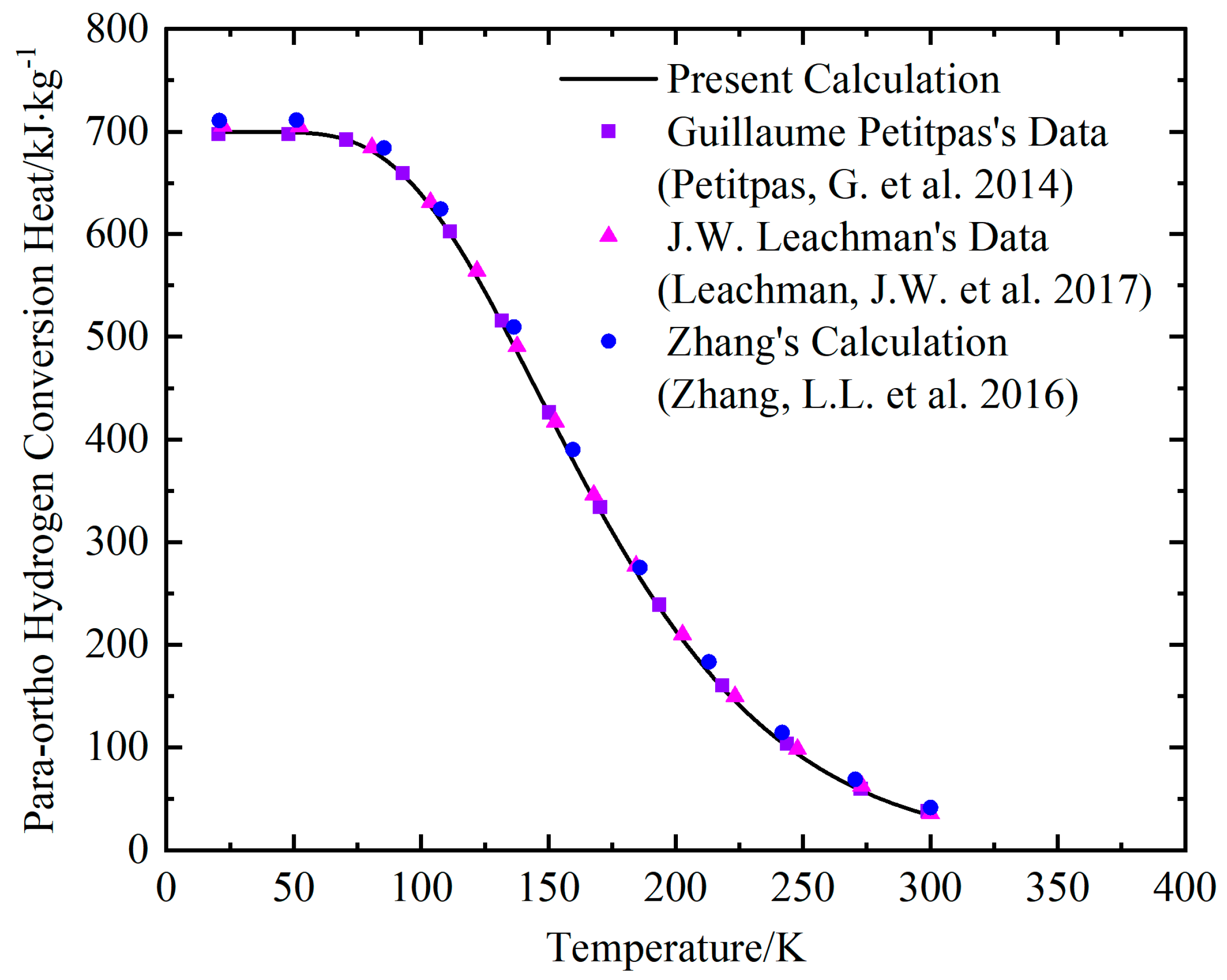
2.1.2. Para-Ortho H₂ Conversion Heat

Since the rotational energy is a different energy form between ortho-H₂ and para-H₂, the para-ortho H₂ conversion heat is the rotational energy difference between a unit mass (1 kg) of ortho-H₂ and para-H₂:

$$q_{\mathrm{po}}=\frac{R}{M}{T}^2\left(\frac{\partial \ln z_{\mathrm{o}}^{\mathrm{r},\mathrm{n}}}{\partial T}-\frac{\partial \ln z_{\mathrm{p}}^{\mathrm{r},\mathrm{n}}}{\partial T}\right)$$

(4)

where R is the universal gas constant, and M is the molar mass of hydrogen molecules.

2.1.3. Isobaric Heat Capacity

The ideal gas heat capacity equation of hydrogen can be written as [5,19]

$$\frac{c_{\mathrm{p}}M}{R}=2.5+{\displaystyle \sum _{k=1}^N{u}_k{\left(\frac{v_k}{T}\right)}^2\frac{\exp \left(v_k/T\right)}{{\left[\exp \left(v_k/T\right)-1\right]}^2}}$$

(5)

where u_k and ν_k are parameters and coefficients of this equation. Their values are given in Reference [5].

2.1.4. Fundamental EOSs for Hydrogen

Leachman [1,5,16] has conducted many studies on the fundamental EOSs of hydrogen, and deduced the expressions of properties such as enthalpy, entropy and heat capacity from these EOSs. The fundamental EOSs for para-H₂, ortho-H₂ and normal H₂ are explicit in the reduced Helmholtz free energy [5,19]:

$$\alpha \left(\delta ,\tau \right)={\alpha }^0\left(\delta ,\tau \right)+{\alpha }^{\mathrm{r}}\left(\delta ,\tau \right)$$

(6)

$$\delta =\frac{{\rho }_{\mathrm{m}}}{{\rho }_{\mathrm{m},\mathrm{c}}} \tau =\frac{T_{\mathrm{c}}}{T}$$

where α(δ,τ) is the reduced Helmholtz free energy; α⁰(δ,τ) is the ideal gas Helmholtz free energy; α^r(δ,τ) is the residual gas Helmholtz free energy; δ and τ are the reduced density and reciprocal reduced temperature. The expression of the molar density can be deduced from the ideal gas EOS:

$${\rho }_{\mathrm{m}}=\frac{n}{V}=\frac{p}{RT}$$

(7)

where n, V, p and T are the amount of substance in mol, volume in m³, pressure in Pa and temperature in K, respectively.

A computationally convenient parameterized form of the ideal gas Helmholtz free energy is [5]

$${\alpha }^0\left(\delta ,\tau \right)=\ln \delta +1.5\ln \tau +a_1+a_2\tau +{\displaystyle \sum _{k=3}^N{a}_k\ln \left[1-\exp \left(b_k\tau \right)\right]}$$

(8)

where the subscript k is the index of each term in the ideal gas heat capacity equation. The coefficients a_k and b_k in the equation of the ideal gas Helmholtz free energy are reported in Reference [5].

The residual gas Helmholtz free energy is [5]

$$\begin{array}{cc}\hfill {\alpha }^{\mathrm{r}}\left(\delta ,\tau \right)& ={\displaystyle \sum _{i=1}^l{N}_i{\delta }^{d_i}{\tau }^{t_i}}+{\displaystyle \sum _{i=l+1}^m{N}_i{\delta }^{d_i}{\tau }^{t_i}\exp \left(-{\delta }^{p_i}\right)}\hfill \\ & +{\displaystyle \sum _{i=m+1}^n{N}_i{\delta }^{d_i}{\tau }^{t_i}\exp \left[{\phi }_i{\left(\delta -D_i\right)}^2+{\beta }_i{\left(\tau -{\gamma }_i\right)}^2\right]}\hfill \end{array}$$

(9)

where l = 7, m = 9, n = 14. All parameters and coefficients of the residual gas Helmholtz free energy are given in Reference [5].

Enthalpy can be derived from the reduced Helmholtz free energy [16]:

$$h=\frac{RT}{M}\left[1+\tau \left({\alpha }_{\tau }^0+{\alpha }_{\tau }^{\mathrm{r}}\right)+\delta {\alpha }_{\delta }^{\mathrm{r}}\right]$$

(10)

where ${\alpha }_{\tau }^0$ is the partial derivative of the ideal gas Helmholtz free energy with respect to τ; ${\alpha }_{\tau }^{\mathrm{r}}$ is the partial derivative of the residual gas Helmholtz free energy with respect to τ; ${\alpha }_{\delta }^{\mathrm{r}}$ is the partial derivative of the residual gas Helmholtz free energy with respect to δ.

Considering that ortho-H₂ has higher energy than para-H₂, the reference enthalpy of ortho-H₂ at its standard boiling point should be adjusted from 0 kJ·kg⁻¹ to 702.98 kJ·kg⁻¹ to show an accurate energy relationship between ortho-H₂ and para-H₂ [5]. Therefore, a correction term 702.98 kJ·kg⁻¹ must be added after the ortho-H₂ enthalpy is calculated by Equation (10).

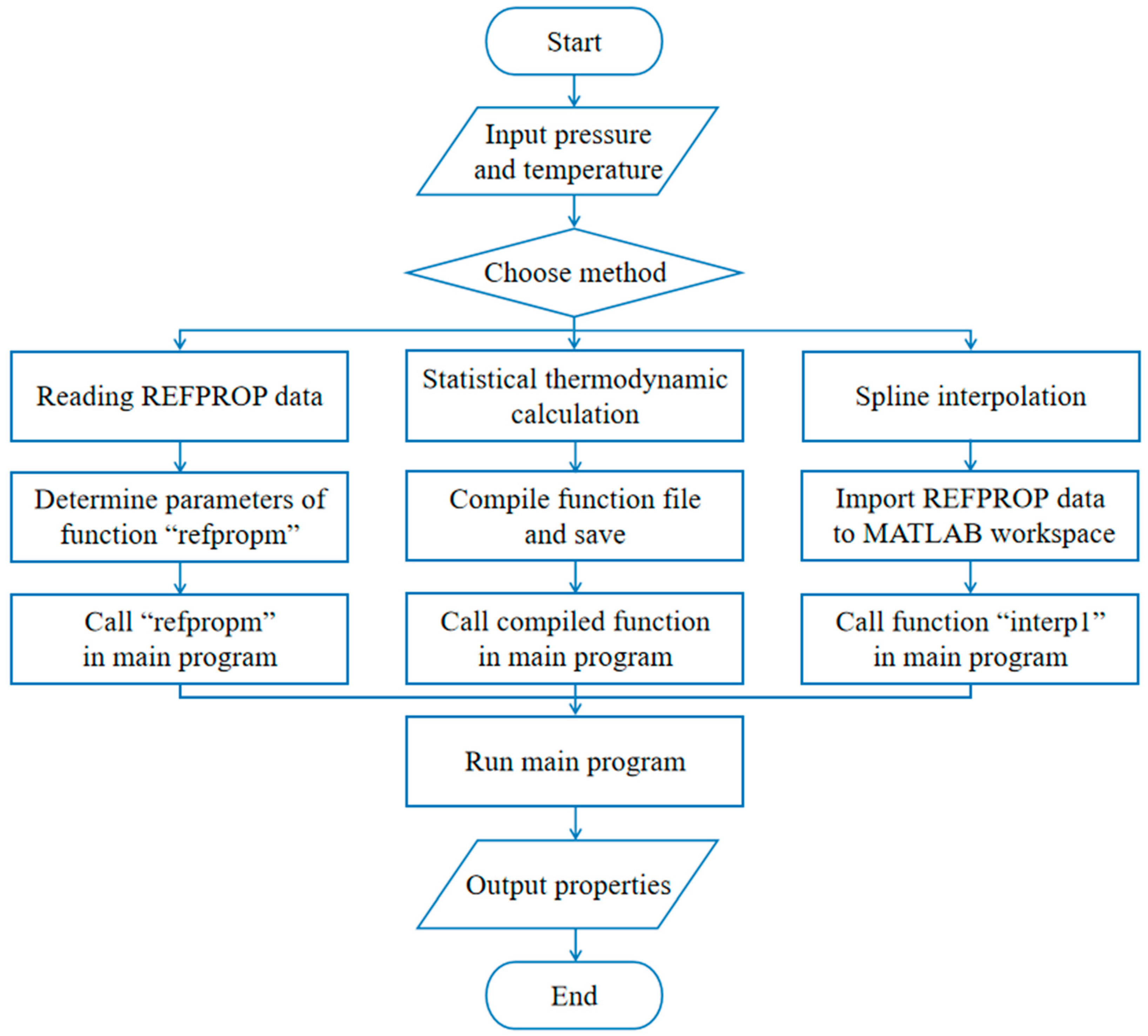
2.2. Implementation of Different Methods for Hydrogen’s Thermophysical Properties

Based on the model in Section 2.1, statistical thermodynamic calculation can be implemented by developing MATLAB programs for determining hydrogen’s thermophysical properties. For example, a function file can be compiled based on Equations (6)–(10) in the compiler of MATLAB to obtain para-H₂ enthalpy at a certain pressure and temperature. The pressure and temperature are the two independent variables of the function, and para-H₂ enthalpy, the required thermophysical property, is set as the dependent variable. After the function compilation is finished, the function file should be saved. As long as the function name and the values of the independent variables are given, the function can be called in a main program by assigning the function value to a variable representing the required property. After the main program runs, the variable can be output and saved in the workspace of MATLAB.

Reading REFPROP data is another common method for determining thermophysical properties by calling the function “refpropm” in a MATLAB program. The parameters of the function include the required property, temperature, pressure and the fluid type. They are sequenced from left to right after “refpropm”. The value of “refpropm” is determined by the given parameters in REFPROP, and it will be returned as a variable representing the property after the program runs. It is worth noting that the interaction between MATLAB and REFPROP may slow down the running speed of the computational program.

Spline interpolation is also employed for determining hydrogen properties. The process of spline interpolation is divided into two steps: (1) acquiring property data from REFPROP in 1 K increments and importing them to the MATLAB workspace before the program runs; (2) calling the function “interp1” in the main program to accomplish spline interpolation, and choosing the fourth parameter of “interp1” as the “spline”. The procedures for determining hydrogen properties using the aforementioned three methods are shown in Figure 1.

Integrating isobaric specific heat (c_p) with temperature is feasible when para-H₂ enthalpy differences between two temperatures are calculated. c_p is obtained via polynomial fitting of REFPROP data, which are given in 1 K increments from 20 K to 300 K.

2.3. Analytical Model for VCS-MLI Combined Structure

2.3.1. Physical Model for VCS-MLI

To compare the statistical thermodynamic method with other methods for determining hydrogen properties, a multilayer insulation (MLI) structure combined with a VCS for liquid hydrogen storage is introduced in Figure 2. The MLI is separated into two parts by the VCS, the inner MLI between the liquid hydrogen tank and the VCS, and the outer MLI between the VCS and the environment. VCS is a metal shield with high thermal conductivity and temperature uniformity. A spiral tube twines around the shield, which serves as a flowing path for the hydrogen vapor vented from the tank [22,23]. As shown in Figure 2, there are three heat fluxes in the VCS-MLI: (1) the heat flux flows into the outer MLI from the warm boundary (q_Total); (2) a part of the heat flux is offset by the VCS (q_VCS); (3) the rest of the heat flux flows through the inner MLI and enters the liquid hydrogen storage tank (q_Tank). The hydrogen vapor is heated when it flows through the VCS tube, and a considerable part of the heat flux from the outer MLI is absorbed by the hydrogen vapor. As a result, q_Tank is much less than q_Total, and better thermal protection for the liquid hydrogen tank can be achieved.

Variable density multilayer insulation (VDMLI) presents a better thermal insulation performance in comparison to the conventional MLI under the same total weight. The physical properties of the VDMLI are presented in

Table 1. Main physical parameters of VDMLI [24].

Physical Parameters of VDMLI	Value
Material of Radiation Shields	Double-Aluminized Mylar
Residual Gas Pressure, p	0.001 Pa
Accomodation Coefficient of Residual Gas, α	0.9
Material of Spacers	Dacron Net
Empirical Coefficient of Spacers, C2	0.008
Relative Density of Spacers, f	0.02
Total Number of Radiation Shields, m	43
Total Number of Spacers, n	126
Total Thickness	33.2 mm
Warm Boundary Temperature, Th	300 K
Cold Boundary Temperature, Tc	20 K

. The configuration of the VDMLI is schemed in Figure 3. VDMLI is normally divided into three zones with the same thickness, the same spacer number, different layer densities and different radiation shield numbers. The numbers of radiation shields and spacers are denoted by m and n, respectively. All configuration parameters of the low-density zone, medium-density zone and high-density zone are marked with subscripts 1, 2 and 3, respectively. The configuration parameters of the VDMLI are listed in

Table 2. Configuration parameters of VDMLI.

Configuration Parameters of VDMLI		Value
Layer Number of Radiation Shields	Low-Layer-Density Zone, m1	8
	Medium-Layer-Density Zone, m2	14
	High-Layer-Density Zone, m3	21
Layer Density	Low-Layer-Density Zone, d1	6.35 N·cm−1
	Medium-Layer-Density Zone, d2	12.70 N·cm−1
	High-Layer-Density Zone, d3	19.35 N·cm−1

, being exactly the same as those of 5#(VD) in Wang’s study [24]. The VCS optimal position is at the midpoint of the VDMLI, as reported in Jiang’s study [22].

2.3.2. VCS-MLI Heat Transfer Model and Its Verification

The heat fluxes in a VCS-MLI must meet the following conservation condition [21,22,25]:

$$Q_1=Q_2+Q_3$$

(11)

where Q₁, Q₂ and Q₃ represent the heat fluxes flowing through the outer MLI, absorbed by hydrogen vapor in the VCS tube, and transferred through the inner MLI to the liquid hydrogen tank. They can be written as [22,26]

$$Q_1=\frac{T_{\mathrm{h}}-T_{\mathrm{VCS}}}{R_{\mathrm{MLI}-\mathrm{out}}}$$

(12)

$$Q_2=\dot{m}\left(h_{\mathrm{out}}-h_{\mathrm{in}}\right)$$

(13)

$$Q_3=\frac{T_{\mathrm{VCS}}-T_{\mathrm{c}}}{R_{\mathrm{MLI}-\mathrm{in}}}$$

(14)

where T_h, T_c and T_VCS are the temperatures of the warm boundary, the cold boundary and the VCS. R_MLI-out and R_MLI-in represent the total thermal resistance of the outer MLI and the inner MLI, which can be acquired using the layer-by-layer (LBL) model [22,24,27,28]. $\dot{m}$ is the mass flow rate of hydrogen vapor in the VCS tube. H_out and h_in are the enthalpies of the hydrogen vapor at the outlet and inlet of the tube. If para-ortho H₂ conversion happens, h is equilibrium H₂ enthalpy. If there is no para-ortho hydrogen conversion, h is para-H₂ enthalpy. In the latter case, the heat flux absorbed in the tube can be calculated as [22]

$$Q_2=\dot{m}{\displaystyle {\int }_{T_{\mathrm{in}}}^{T_{\mathrm{out}}}{c}_{\mathrm{p}}\mathrm{d}T}$$

(15)

where c_p is para-H₂ isobaric heat capacity; T_in and T_out are the temperatures of the tube inlet and outlet, respectively.

The LBL model is verified to calculate the thermal resistances of the inner and outer MLI. The temperature profile is consistent with Wang’s [24] experiment and calculation, as shown in Figure 4. Moreover, the calculated temperature is closer to the experimental data in the low-layer-density zone. The analytical model for the VCS-MLI structure is then validated. A 40 mm thick foam is added between the tank and the cold boundary in accordance with the insulation structure that Jiang [22] studied. Figure 5 shows that the temperature distributions agree well with Jiang’s results [22]. The maximum deviations are not more than 6% whether or not the VCS is applied. The analytical model for the VCS-MLI is applicable to subsequent analysis.

3. Results and Discussion

3.1. Accuracy of Statistical Thermodynamic Method

3.1.1. Ortho-H₂ Fraction and Conversion Heat

The ortho-H₂ fraction in equilibrium H₂ is calculated. As shown in Figure 6, the present calculation agrees well with the data from four scholars [4,19,21,29]. When the temperature exceeds 198 K, the composition of equilibrium H₂ is approximately 75% ortho-H₂ and 25% para-H₂. When the temperature approaches the normal boiling point of liquid hydrogen, almost all of the hydrogen molecules are likely to transfer to the lowest energy level (j = 0) [29]. As para-H₂ molecules are restricted to even rotational energy levels, 99.8% para-H₂ and 0.2% ortho-H₂ comprise equilibrium H₂.

Figure 7 shows the calculated para-ortho H₂ conversion heat. The present calculation is in accordance with the data reported by three scholars [4,19,29]. At low temperatures, para-H₂ molecules tend to be at the most stable energy level (j = 0), so almost all ortho-H₂ molecules are converted to the lowest energy level and extensive energy is released. The para-ortho H₂ conversion heat is maintained above 690 kJ·kg⁻¹ if the temperature is less than 73 K. As the temperature rises, some para-H₂ molecules jump to higher energy levels. Therefore, not all ortho-H₂ molecules need to be transferred to para-H₂ molecules, and the energy released in para-ortho H₂ conversion drops [29]. At elevated temperatures (T > 300 K), all rotational energy levels of hydrogen molecules are populated, and the rotational energy of para-H₂ approaches that of ortho-H₂, so para-ortho H₂ conversion heat tends toward zero.

3.1.2. Isobaric Heat Capacity and Enthalpy

The ideal gas heat capacities of hydrogen are calculated and shown in Figure 8. The hydrogen pressure is set as 0.1 Mpa. The calculation results and REFPROP data are displayed in 1 K increments from 20 K to 300 K. Chen’s [30], Meng’s [21] and Leachman’s [19] data are randomly extracted from their studies. Figure 8a shows that the calculated isobaric heat capacities (c_p) of para-H₂ agree well with all the data and deviate from the REFPROP data within 1% above 60 K. The calculated c_p are consistent with Meng’s [21] and Leachman’s [19] data within 20–60 K, but deviate from REFPROP and Chen’s [30] data below 60 K. The maximum deviation between the calculation and REFPROP data is 14.14% at 20 K. As shown in Figure 8b, the calculated c_p of ortho-H₂ is in good accordance with Meng’s [21] and Leachman’s [19] data. The deviation between the present calculation and REFPROP data is within 1% above 80 K and within 5% above 27 K, but the deviation becomes larger when temperature approaches the normal boiling point. This is because the REEPROP data in Figure 8 are the real gas isobaric heat capacities, but the calculated data are the ideal gas isobaric heat capacities. Para-H₂ and ortho-H₂ cannot be regarded as ideal gases near their normal boiling points. The difference between the real gas and the ideal gas heat capacities becomes larger at lower temperatures. Consequently, there is a deviation between the calculated isobaric heat capacities and the REEPROP data.

The para-H₂ and ortho-H₂ enthalpies are calculated based on the Helmholtz-type fundamental EOS. Figure 9a shows that the calculated para-H₂ enthalpies correspond well with Meng’s [21] and Leachman’s [19] data and have the same tendency as Chen’s [30] data. But the calculated enthalpies differ by about 300 kJ·kg⁻¹ from Chen’s [30] data, which is probably the result of a different selection of the reference state. The deviation between the calculation and REFPROP data reaches its maximum of 2.22% at 20 K and is maintained at less than 0.1% above 25 K. As Figure 9b displays, the ortho-H₂ enthalpies obtained using statistical thermodynamics match Meng’s [21] and Leachman’s [19] data well. However, the ortho-H₂ enthalpies from REFPROP cannot be directly used because REFPROP assumes a default reference state of a saturated liquid at the normal boiling point. The enthalpy of the saturated ortho-H₂ is assumed to be 0 kJ·kg⁻¹, which leads to an inaccurate prediction of ortho-H₂ enthalpies from the original REFPROP data. Ortho-H₂ molecules are restricted to odd energy levels (j = 1) and para-H₂ molecules are restricted to even energy levels (j = 0) at the normal boiling point. Consequently, ortho-H₂ has higher rotational energy than para-H₂. Based on this fact, the reference enthalpy of ortho-H₂ must be changed from 0 kJ·kg⁻¹ to 702.98 kJ·kg⁻¹ to show a correct energy relationship between ortho-H₂ and para-H₂ [19]. After the correction, the calculation is consistent with REFPROP data. The maximum deviation is 0.18% at 20 K.

Table 3. Comparison of calculated para-H₂ enthalpy and REFPROP data under different pressures.

Pressure/Mpa	Maximum Deviation/%
0.5	0.0006
1	0.0021
2	0.0051
5	0.0271
10	0.2454
20	2.3129

shows the comparison between the calculated para-H₂ enthalpies and REFPROP data under different pressures from 0.5 Mpa to 20 Mpa. Temperatures are taken from 100 K to 1500 K in 100 K increments. The deviations are not more than 2.32% even though the pressure rises to 20 Mpa. This indicates that the statistical thermodynamic method is also applicable at higher temperatures and pressures.

So far, the statistical thermodynamic method for determining the thermophysical properties of hydrogen has been proved to be accurate. This method is applicable for the determination of hydrogen’s thermophysical properties.

3.2. Convenience of the Statistical Thermodynamic Method

Convenience is another advantage of the statistical thermodynamic method. Three tests are conducted on the same computer with MATLAB 2022a to assess the convenience of the statistical thermodynamic method. The running speeds of programs under different methods for determining hydrogen’s thermophysical properties are compared. To guarantee that all methods for determining hydrogen’s thermophysical properties are compared under the same conditions, no parallel toolbox calculations or other acceleration modules are used in any of calculations, so that the interference of all acceleration measures in computational speed can be eliminated. During these tests, the computer maintains the same operating conditions. The hardware characteristics of the computer described in the present study are as follows: the volume and frequency of RAM are 16.0 GB and 2.60 GHz, respectively; the type of CPU is 11th Gen Intel(R) Core(TM) i5-11400F; the type of GPU is NVIDIA GeForce GT 730. The most direct way to judge the running speed of a MATLAB program is to measure its running time by adding “tic” and “toc” (two timing functions of MATLAB) to the start and the end of the program, respectively. “toc” reads the elapsed time expressed in seconds since the stopwatch timer started by the call to the “tic” function. If the running time is much less than 0.1 s, the program will run too fast for “tic” and “toc” to provide useful data. In this case, the timed section in the program must be run in a loop, and the total running time of the loop is measured. To ensure the reliability of measuring the running time, every program under a specific method must be run 20 times under the same condition. The average running time indicates the running speed of the program.

The first test is to calculate para-H₂ enthalpies at 0.1 MPa from 20 K to 300 K in 0.02 K or 0.01 K increments, and the corresponding circulation numbers are 14,001 and 28,001, respectively. The comparison of the running speeds of programs with three methods is listed in

Table 4. Average running time of para-H₂ enthalpy calculation programs.

Method	Average Running Time/s (14,001 Circulations)	Average Running Time/s (28,001 Circulations)
Spline Interpolation	0.1735	0.3356
REFPROP Data	1.6971	3.3626
Statistical Thermodynamic Calculation	0.0716	0.1463

. It is indicated that reading REFPROP data in a program for para-H₂ enthalpy calculation is the most time-consuming, requiring about 23 times as much time as statistical thermodynamic calculation. Statistical thermodynamic calculation can save much more time if the circulation numbers are multiplied.

The second test is to calculate the heat absorption of the hydrogen vapor in a VCS tube, or the hydrogen enthalpy difference at the outlet and inlet of the tube. The inlet temperature is 20 K. The outlet temperature varies from 100 K to 300 K in 0.02 K or 0.01 K increments, and the corresponding circulation numbers are 10,001 or 20,001. Two cases are considered: (1) the hydrogen vapor always maintains an equilibrium state if para-ortho H₂ conversion is employed; (2) the hydrogen vapor contains para-H₂ if para-ortho H₂ conversion is not employed.

Table 5. Average running time of programs for calculating hydrogen enthalpy differences.

Case	Method	Average Running Time/s (10,001 Circulations)	Average Running Time/s (20,001 Circulations)
With Para-ortho Conversion	Spline Interpolation (1.1)	0.3253	0.6562
	REFPROP Data (1.2)	56.8849	113.5774
	Statistical Thermodynamic Calculation (1.3)	0.1077	0.2124
Without Para-ortho Conversion	Spline Interpolation (2.1)	0.1731	0.3384
	REFPROP Data (2.2)	1.2122	2.3988
	Integral of cp with Temperature (2.3)	81.5196	163.1697
	Statistical Thermodynamic Calculation (2.4)	0.0518	0.1039

shows that much more time is consumed with the methods of calling enthalpy data from REFPROP and integrating c_p. It is worth noting that acquiring equilibrium H₂ enthalpies is much more time-consuming than acquiring para-H₂ enthalpies. Therefore, reading REFPROP data is not recommended when para-ortho H₂ conversion is considered. Statistical thermodynamic calculation, however, is more efficient and faster. Whether para-ortho H₂ conversion is considered or not, the statistical thermodynamic method saves the most time. For instance, the average running time of the program with Method 1.3 is about 33% that of the program with Method 1.1 and about 0.18% that of the program with Method 1.2.

The third test is to calculate the thermal insulation performance of the VCS-VDMLI structure. The running speeds of the entire calculation procedure with different methods are compared. The VCS temperature is set as a loop variable. The initial VCS temperature is 60 K, and the VCS temperature increases 0.01 K after each loop. The iteration stops when three heat fluxes in the VCS-VDMLI meet the conservation condition in Equation (11) and the temperature profile of the VDMLI no longer changes with iterations. The test results are shown in

Table 6. Average running time of programs for calculating VCS-VDMLI performances.

Case	Method	Average Running Time/s	Number of Iterations
With Para-ortho Conversion	Spline Interpolation (1.1)	0.2668	5198
	REFPROP Data (1.2)	37.0464	5224
	Statistical Thermodynamic Calculation (1.3)	0.1030	5182
Without Para-ortho Conversion	Spline Interpolation (2.1)	0.1947	6108
	REFPROP Data (2.2)	1.0806	6137
	Integral of cp with Temperature (2.3)	15.3030	6102
	Statistical Thermodynamic Calculation (2.4)	0.0859	6090

. It can be found that the statistical thermodynamic method still saves the most time when the numbers of iterations are about the same. The average running time of the program with Method 1.3 is about 0.28% that of the program with Method 1.2. Although spline interpolation costs much less time than reading REFPROP data, the running time is more than twice that of statistical thermodynamic calculation.

It can be found that the statistical thermodynamic method is feasible and efficient in engineering practice. The developed computational programs based on this method can be adopted when hydrogen’s thermophysical properties are needed. In addition to accuracy and convenience, the statistical thermodynamic method based on explicit Helmholtz free energy EOSs has thermodynamic unity. Thermophysical properties, such as enthalpy, entropy, specific heat capacity, speed of sound, etc., can be obtained by taking first-order or at most second-order derivatives of the Helmholtz free energy with respect to temperature or density, which is much simpler than calculating enthalpies from integrals using EOSs explicit in pressure. The programs for determining thermophysical properties of different fluids have the same frame. All the coefficients in the reduced Helmholtz free energy equations are known. They can be written as elements in arrays and conveniently replaced when the fluid changes.

4. Conclusions

A statistical thermodynamic model for determining the thermophysical properties of hydrogen is implemented by developing computational programs. Properties include ortho-H₂ fraction in equilibrium H₂, para-ortho H₂ conversion heat, ideal gas isobaric heat capacities and enthalpies of ortho-H₂ and para-H₂. A function file for determining thermophysical properties can be compiled in the MATLAB compiler and called when the main program is running.

Hydrogen properties are calculated using the developed programs. At 0.1 MPa, para-H₂ isobaric heat capacities show deviations from REFPROP data within 5% above 29 K. The deviation of para-H₂ enthalpies from REFPROP data is not more than 0.1% above 25 K, and reaches its maximum of 2.22% at 20 K. The deviations of para-H₂ enthalpies between the present calculation and REFPROP data are all within 2.32% in the region between 100 K and 1500 K at pressures up to 20 MPa. Considering that ortho-H₂ has higher energy than para-H₂, the reference enthalpy of ortho-H₂ at its normal boiling point should be adjusted to 702.98 kJ·kg⁻¹. The deviations of calculated ortho-H₂ enthalpies from corrected REFPROP data are within 0.18%. The accuracy of the statistical thermodynamic method is validated.

To illustrate the convenience of the statistical thermodynamic method, three methods, including spline interpolation, reading REFPROP data and statistical thermodynamic calculation, are compared. The average running time of the programs with the statistical thermodynamic method is 4.3%, 0.18%, 0.28% and 7.95% that of the program with the method of reading REFPROP data when para-H₂ enthalpies, equilibrium H₂ enthalpy differences and the performances of the VCS-MLI structure with and without para-ortho H₂ conversion are calculated, respectively. The developed computational programs based on the statistical thermodynamic model are applicable and efficient in engineering practice.

References

1. Jacobsen, R.T.; Leachman, J.W.; Penoncello, S.G.; Lemmon, E.W. Current status of thermodynamic properties of hydrogen. Int. J. Thermophys. J. Thermophys. Prop. Thermophys. Its Appl. 2007, 28, 758–772. [Google Scholar] [CrossRef]
2. Barthelemy, H.; Weber, M.; Barbier, F. Hydrogen storage: Recent improvements and industrial perspectives. Int. J. Hydrogen Energy 2017, 42, 7254–7262. [Google Scholar] [CrossRef]
3. Aziz, M. Liquid Hydrogen: A review on liquefaction, storage, transportation, and safety. Energies 2021, 14, 5917. [Google Scholar] [CrossRef]
4. Petitpas, G.; Aceves, S.M.; Matthews, M.J.; Smith, J.R. Para-H2 to ortho-H2 conversion in a full-scale automotive cryogenic pressurized hydrogen storage up to 345 bar. Int. J. Hydrogen Energy 2014, 39, 6533–6547. [Google Scholar] [CrossRef]
5. Leachman, J.W.; Jacobsen, R.T.; Penoncello, S.G.; Lemmon, E.W. Fundamental equations of state for parahydrogen, normal hydrogen, and orthohydrogen. J. Phys. Chem. Ref. Data 2009, 38, 721–748. [Google Scholar] [CrossRef]
6. Nasrifar, K. Comparative study of eleven equations of state in predicting the thermodynamic properties of hydrogen. Int. J. Hydrogen Energy 2010, 35, 3802–3811. [Google Scholar] [CrossRef]
7. Sakoda, N.; Shindo, K.; Shinzato, K.; Kohno, M.; Takata, Y.; Fujii, M. Review of the thermodynamic properties of hydrogen based on existing equations of state. Int. J. Thermophys. J. Thermophys. Prop. Thermophys. Its Appl. 2010, 31, 276–296. [Google Scholar] [CrossRef]
8. Redlich, O.; Kwong, J.N. On the thermodynamics of solutions. V. An equation of state. Fugacities of gaseous solutions. Chem. Rev. 1949, 44, 233–244. [Google Scholar] [CrossRef]
9. Goodwin, R.D.; Diller, D.E.; Roder, H.M.; Weber, L.A. Second and third virial coefficients for hydrogen. J. Res. Natl. Bur. Stand. Sect. A Phys. Chem. 1964, 68, 121. [Google Scholar] [CrossRef]
10. Goodwin, R.D.; Diller, D.E.; Roder, H.M.; Weber, L.A. Pressure-density-temperature relations of fluid para hydrogen from 15 to 100 K at pressures to 350 atmospheres. J. Res. Natl. Bur. Stand. Sect. A Phys. Chem. 1963, 67, 173–192. [Google Scholar] [CrossRef]
11. Goodwin, R.D. An equation of state for fluid parahydrogen from the triple-point to 100 °K at pressures to 350 atmospheres. J. Res. Natl. Bur. Stand. Sect. A Phys. Chem. 1967, 71A, 203–212. [Google Scholar] [CrossRef] [PubMed]
12. Mccarty, R.D.; Weber, L.A. Thermophysical Properties of Parahydrogen from the Freezing Liquid Line to 5000 R for Pressures to 10,000 psia; NASA Center for Aerospace Information (CASI): Hanover, MD, USA, 1972.
13. McCarty, R.D. A Modified Benedict-Webb-Rubin Equation of State for Parahydrogen; National Bureau of Standards: Gaithersburg, MD, USA, 1974.
14. Younglove, B.A. Thermophysical Properties of Fluids. I. Argon, Ethylene, Parahydrogen, Nitrogen, Nitrogen Trifluoride, and Oxygen; National Standard Reference Data System: Boulder, CO, USA, 1982.
15. Jacobsen, R.T.; Stewart, R.B.; Jahangiri, M.; Penoncello, S.G. A New Fundamental Equation for Thermodynamic Property Correlations; Springer: Boston, MA, USA, 1986. [Google Scholar]
16. Jacobsen, R.T.; Penoncello, S.G.; Lemmon, E.W. Current status of thermodynamic properties of cryogenic fluids. Adv. Cryog. Eng. 1998, 43, 1273–1280. [Google Scholar]
17. Kunz, O.; Klimeck, R.; Wagner, W.; Jaeschke, M. The GERG-2004 Wide-Range Equation of State for Natural Gases and Other Mixtures; U.S. Department of Energy Office of Scientific and Technical Information: Oak Ridge, TN, USA, 2007.
18. Kunz, O.; Wagner, W. The GERG-2008 wide-range equation of state for natural gases and other mixtures: An expansion of GERG-2004. J. Chem. Eng. Data 2012, 57, 3032–3091. [Google Scholar] [CrossRef]
19. Leachman, J.W.; Jacobsen, R.T.; Lemmon, E.W.; Penoncello, S.G. Thermodynamic Properties of Cryogenic Fluids; Springer: Cham, Switzerland, 2017. [Google Scholar]
20. Bliesner, R.M. Parahydrogen-Orthohydrogen Conversion for Boil-Off Reduction from Space Stage Fuel Systems. Ph.D. Thesis, Washington State University, Pullman, WA, USA, 2013. [Google Scholar]
21. Meng, C.J.; Zhang, L.; Huang, Y.H. Analysis of cooling effect of para-ortho hydrogen conversion in vapor cooling shield. Vac. Cryog. 2022, 28, 279–284. [Google Scholar] [CrossRef]
22. Jiang, W.B.; Zuo, Z.Q.; Huang, Y.H.; Wang, B.; Sun, P.J.; Li, P. Coupling optimization of composite insulation and vapor-cooled shield for on-orbit cryogenic storage tank. Cryogenics 2018, 96, 90–98. [Google Scholar] [CrossRef]
23. Jiang, W.B.; Sun, P.J.; Li, P.; Zuo, Z.; Huang, Y. Transient thermal behavior of multi-layer insulation coupled with vapor cooled shield used for liquid hydrogen storage tank. Energy 2021, 231, 120859. [Google Scholar] [CrossRef]
24. Wang, B.; Huang, Y.H.; Li, P.; Sun, P.J.; Chen, Z.C.; Wu, J.Y. Optimization of variable density multilayer insulation for cryogenic application and experimental validation. Cryogenics 2016, 80, 154–163. [Google Scholar] [CrossRef]
25. Shi, C.Y.; Zhu, S.L.; Wan, C.C.; Bao, S.; Zhi, X.; Qiu, L.; Wang, K. Performance analysis of vapor-cooled shield insulation integrated with para-ortho hydrogen conversion for liquid hydrogen tanks. Int. J. Hydrogen Energy 2023, 48, 3078–3090. [Google Scholar] [CrossRef]
26. Zheng, J.P.; Chen, L.B.; Wang, J.; Xi, X.; Zhu, H.; Zhou, Y.; Wang, J. Thermodynamic analysis and comparison of four insulation schemes for liquid hydrogen storage tank. Energy Convers. Manag. 2019, 186, 526–534. [Google Scholar] [CrossRef]
27. Brown, T.M.; Hastings, L.J.; Hedayat, A. Analytical Modeling and Test Correlation of Variable Density Multilayer Insulation for Cryogenic Storage; NASA Center for Aerospace Information (CASI): Hanover, MD, USA, 2004.
28. Huang, Y.H.; Wang, B.; Zhou, S.H.; Wu, J.; Lei, G.; Li, P.; Sun, P. Modeling and experimental study on combination of foam and variable density multilayer insulation for cryogen storage. Energy 2017, 123, 487–498. [Google Scholar] [CrossRef]
29. Zhang, L.L.; Sun, Q.G.; Gao, X.; Liu, Y.Y.; Jiang, Y.M. Statistical thermodynamics analysis of hydrogen ortho-para conversion matters. Chin. J. Low Temp. Phys. 2016, 38, 81–84. [Google Scholar]
30. Chen, G.B.; Huang, Y.H.; Bao, R. Thermophysical Properties of Cryogenic Fluids; National Defense Industry Press: Beijing, China, 2006. [Google Scholar]
Figure 1. Procedures for determining hydrogen properties using different methods.
Applsci 13 07466 g001
Figure 2. Schematic of VCS-MLI combined structure.
Applsci 13 07466 g002
Figure 3. Diagram of VDMLI configuration.
Applsci 13 07466 g003
Figure 4. Temperature profiles in VDMLI [24].
Applsci 13 07466 g004
Figure 5. Comparison of temperature profiles in VDMLI/VCS-VDMLI [22].
Applsci 13 07466 g005
Figure 6. Equilibrium ortho-H2 fraction versus temperature [4,19,21,29].
Applsci 13 07466 g006
Figure 7. Para-ortho H2 conversion heat versus temperature [4,19,29].
Applsci 13 07466 g007
Figure 8. Isobaric heat capacity versus temperature: (a) para-H2; (b) ortho-H2 [19,21,30].
Applsci 13 07466 g008
Figure 9. Enthalpy versus temperature: (a) para-H2; (b) ortho-H2 [19,21,30].
Applsci 13 07466 g009