2.1. Two–Layered Strip Foundation Failure Mode
In terms of the different soil characteristics of a two–layered strip foundation, this paper makes the following assumptions before analyzing the bearing capacity of the foundation:
The two–layered soils are assumed as elastic–perfectly plastic material, and the soils above the base level are simplified as overload q on both sides of the foundation.
Two–layered soils are subjected to the associated flow rule and Mohr–Coulomb yield criterion.
The foundation is assumed to be relatively still, and its base surface is assumed to be completely rough.
The foundation moves downward at an assumed vertical speed .
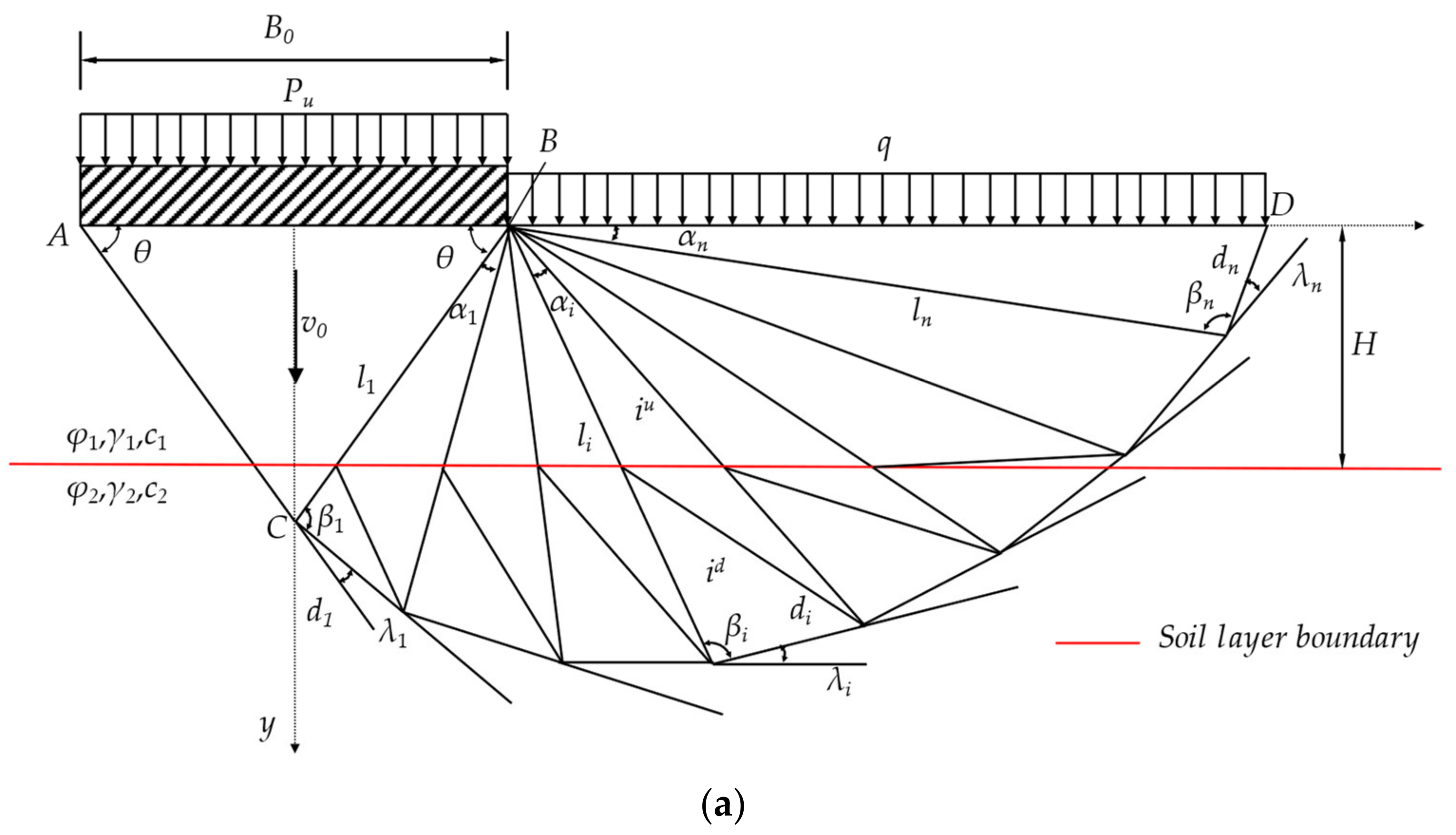
Based on the above assumptions, a planar kinematically permissible multi–block failure mechanism under vertical uniform load is established (Take the right half for a diagram), as shown in
Figure 1a.
B0 is the width of the strip footing,
H is the thickness of the upper soil,
Pu is the vertical uniformly distributed load,
q is the overload on both sides, and
v0 is the vertical downward speed of the strip foundation.
,
,
and
,
,
are the internal friction angle, soil weight, and cohesion of the upper and lower soil, respectively. In this model, the base angle of the isosceles triangle is marked as
θ, and base edge length is
B0. Starting from the rigid block
ABC, the remaining rigid blocks are numbered to the nth block in turn from the left to right. For each rigid block, its angle variable is recorded as
(
i = 1, 2, 3, …,
n),
(
i = 1, 2, 3, …,
n), and the side length is recorded as
(
i = 1, 2, 3, …,
n),
(
i = 1, 2, 3, …,
n). The side length can be calculated through the geometric relationship of triangles, and the area of each rigid block is recorded as
,
(
i = 1, 2, 3, …,
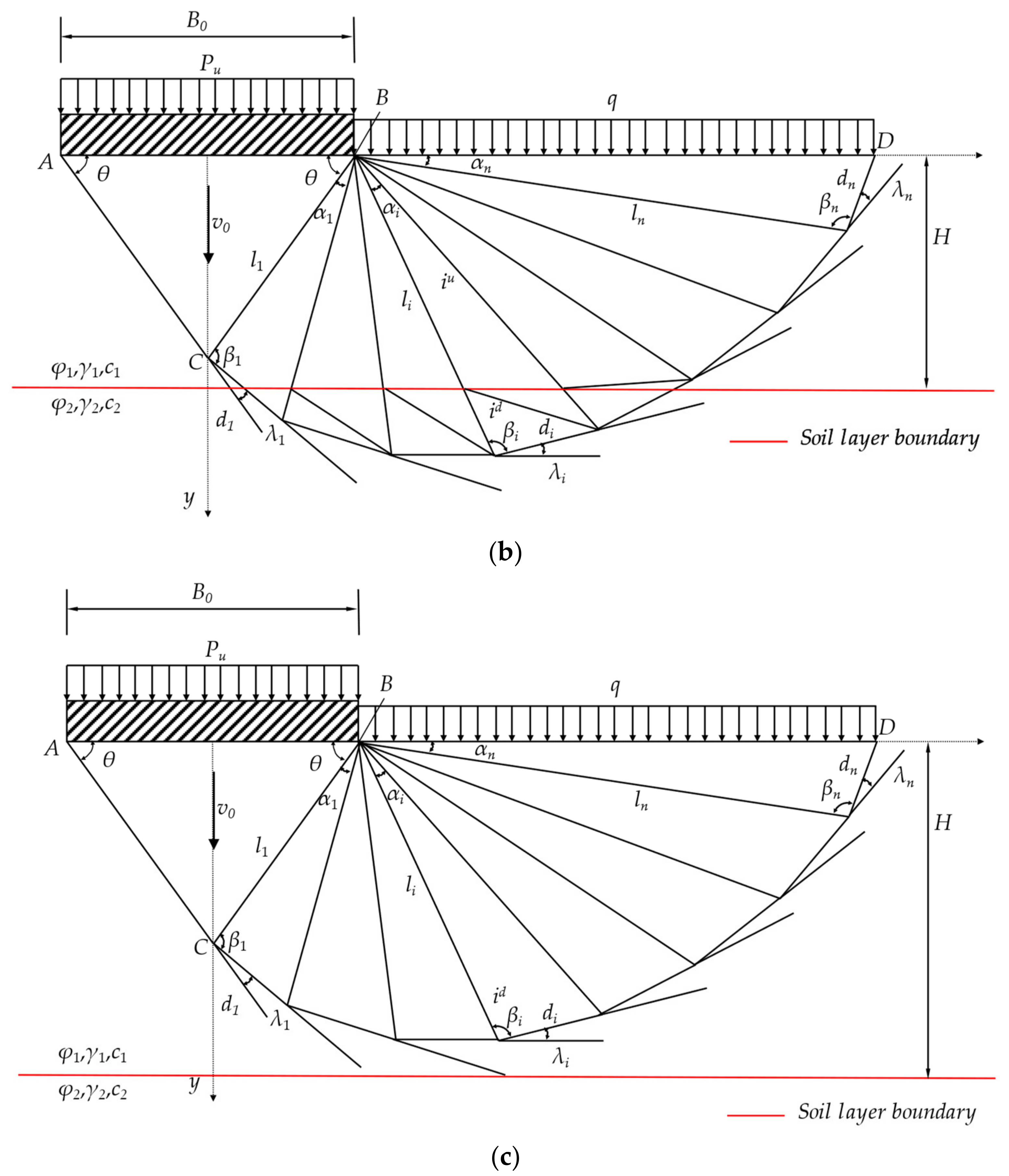
n). It should be mentioned that, due to the uncertain position of the soil layer boundary, the multi–rigid block failure mechanisms for the two–layered strip foundation are discussed with three cases herein. The soil layer boundary passes through the stiff block
ABC in the first case, which is depicted in
Figure 1a. The second case is that the soil layer boundary line does not pass through rigid block
ABC but passes through some subsequent rigid blocks, which is depicted in
Figure 1b. The third case is that the soil layer boundary is completely placed under the foundation failure mechanism, as shown in
Figure 1c.
Since the weight of the upper and lower soil layers is different, it is necessary to calculate the gravity of the rigid block of different soil layers. Thus, the superscripts u (up), m (middle), and d (down) are used to differ the variables of the rigid block in the upper and lower soil layers, respectively.
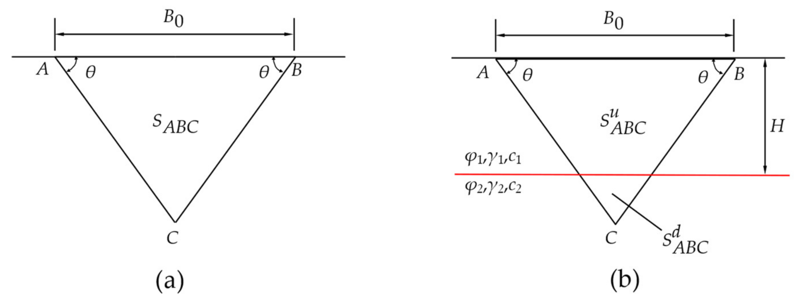
The rigid blocks in the multi–rigid block failure mechanism of the two–layered strip foundation are divided into three types to calculate their area. The rigid block ABC is Type I. The failure mechanism of a stiff block of Type II only penetrates the top layer of soil, while that of Type III penetrates two soil layers.
- (1)
Type I
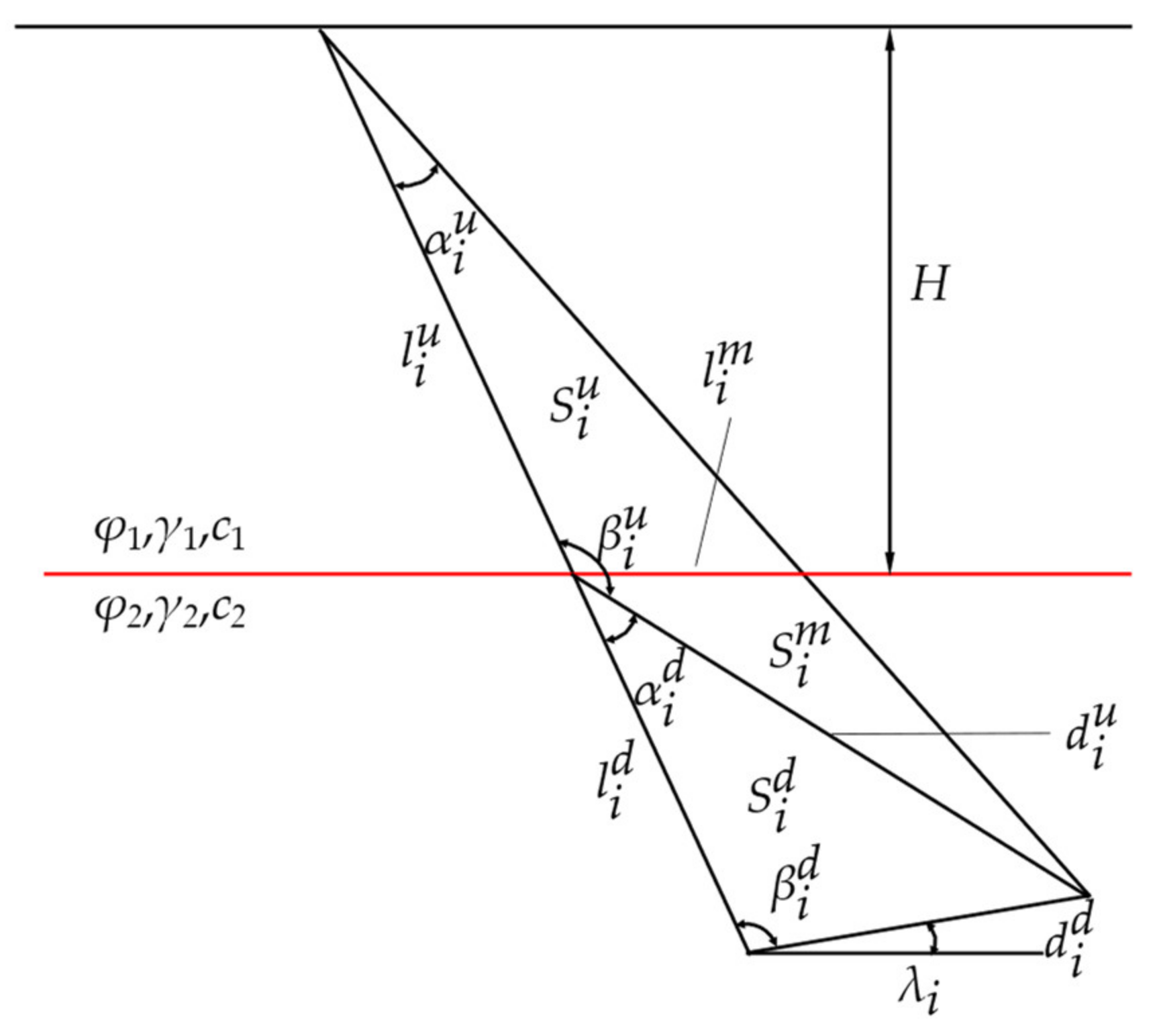
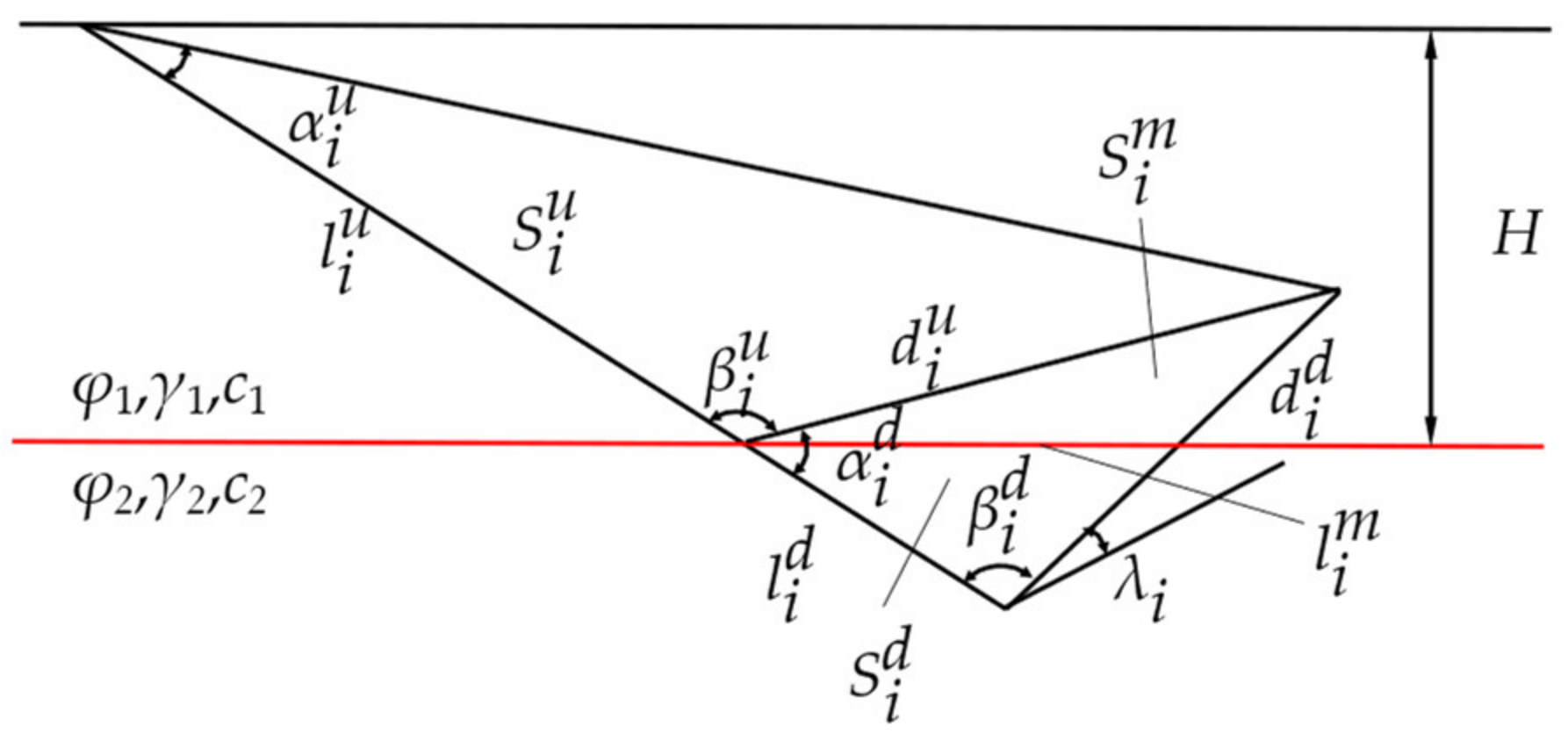
When calculating Type I, there are two cases, that is, whether Type I passes through the upper and lower soil layers at the same time, as shown in
Figure 2a,b.
It is necessary to determine whether the rigid block
ABC passes through the two layers soil by Equation (1). If Equation (1) is valid, Type I passes through the two–layered soil, and is calculated according to
Figure 2a. The area expression is shown in Equation (2), otherwise, Type I does not pass through the two–layered soil. It is calculated according to
Figure 2b, and the area expression is shown in Equation (3).
where
represents the area of the rigid block in
Figure 2a.
represents the area containing only upper soil in
Figure 2b.
represents the area of the lower triangle in
Figure 2b.
- (2)
Type II and Type III
For other rigid blocks
i except for Type I, it is necessary to determine whether the rigid block belongs to Type II or Type III by Equation (4). When Equation (4) is valid, it means that the rigid block
i passes through the two–layered soil, which belongs to Type III. The rigid block needs to be divided into two rigid blocks, namely,
iu and
id, for calculation. Otherwise, it means that the rigid block
i belongs to Type II, which can be calculated directly.
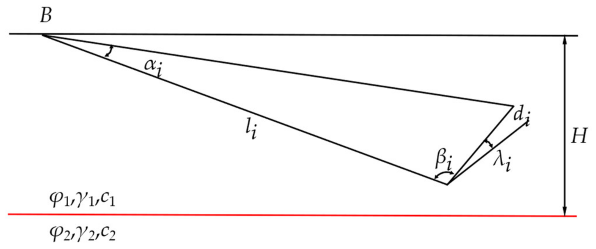
The triangular rigid block
i of Type II is shown in
Figure 3, and its variable expression is shown in Equation (5):
where
li and
di represent the two side lengths of the rigid block
i, and
Si represents the area of the rigid block
i.
For the triangular rigid block of Type III, the rigid block
id is composed of a triangle. Since the rigid block
iu is in two layers of soil, it will be divided into two areas, namely,
and
, as shown in
Figure 4. The area expression such as Equations (6)–(8):
where the parameters with superscripts
u and
d represent the parameters on the corresponding small rigid block after the rigid block of Type III is divided into upper and lower rigid blocks
iu and
id.
is the length of the soil layer boundary line passing through the
rigid block.
refers to the area where the
rigid block belongs to the upper soil.
is the area of the
iu rigid block that belongs to the subsoil.
is the area of the
id rigid block.
The transition of two types of different rigid blocks needs to be calculated separately, as shown in
Figure 5. It means that the area formula will be different from the above situation when the type III rigid block is transformed into a Type II rigid block.
means that the soil layer where the area is located has changed, but the solution idea is similar, so it will not be repeated here.
2.2. Establishment of the Permissible Velocity Field
To do an upper-bound analysis of strip footing under vertical uniform load, a flexible permitted velocity field must be created for each rigid block. The allowable velocity field can be determined using the triangular geometric relationship of the allowable velocity field. The absolute and relative velocity vectors of three types of rigid blocks are analyzed and solved, respectively:
In Equations (9)–(33), the internal friction angle of the upper soil is φ1. The internal friction angle of the soil is φ2. θ is the bottom angle of rigid block ABC. is the sum of i − 1 triangle the rigid block’s top angle before rigid block i. is the bottom angle β of rigid block iu. , and represents the absolute velocity vector direction angle of rigid block i, rigid block id, and rigid block iu, where is determinable. , and represents the absolute velocity vector of rigid block i, rigid block id, and rigid block iu. The relative speed between the two rigid blocks, i − 1 and i, is represented by . The expression of relative velocity between the other rigid blocks is similar, so it will not be repeated.
When the two–layered strip foundation fails, rigid block ABC of Type I is designed to travel vertically downward at a speed of v0.
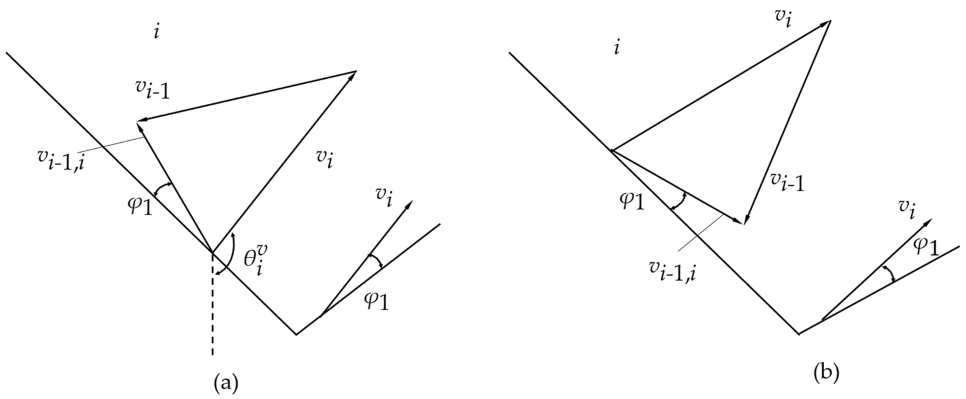
During the analysis of Type II, due to the uncertainty of the relative motion direction between rigid blocks, there are two cases of compatible velocity relationship between rigid blocks
i and rigid blocks
i − 1, as shown in
Figure 6.
According to the compatible velocity vector triangle in two cases, we can calculate vi−1,i using the Equations (9) and (10) or the Equations (11) and (12).
For
Figure 6a, the relative velocity
between rigid blocks
i and
i − 1 face upwards along the velocity discontinuity and form an angle
φ1.
Equation (11) applies to case: II −1: (
Figure 6a):
In the second case in
Figure 6b, the relative velocity
vi−1,i between rigid blocks
i − 1 and
i face downward along the velocity discontinuity
φ1.
To make Equations (12) and (13) work, the following requirements need to be met:
It should be noted that when the rigid block (i − 1) belongs to Type III, that is, at the joint of two types of rigid blocks, in the above formula should be changed to for calculation.
The velocity vector solution of Type III shall be divided into two rigid blocks: iu and id. Rigid block iu and id are, respectively, the upper and the lower parts of each rigid block i of Type III separated by the intersection of the boundary line of the foundation soil layer and the triangle edge connecting the vertex of the triangle. In the calculation process, it is necessary to analyze the permissible velocity relationship between rigid block i − 1u and rigid block id, rigid block i − 1u and rigid block iu, rigid block id and rigid block iu. Then, the relative velocity of rigid block iu and id are solved simultaneously through the permissible velocity relation.
Type III–id:
According to the relationship of permissible velocity between rigid block
i − 1
u and
id, the direction angle of the velocity vector of rigid block
id can be obtained as Equation (15).
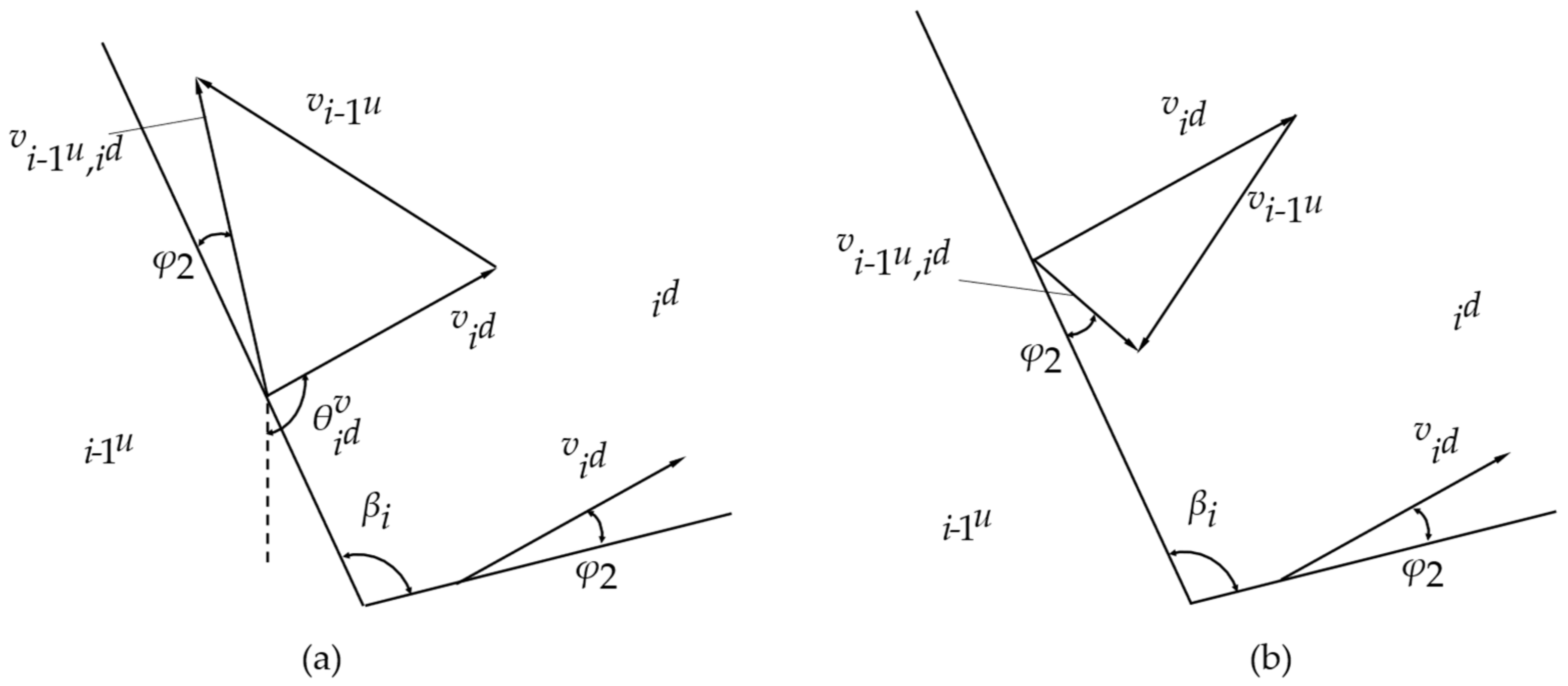
As shown in
Figure 7, there are two cases of permissible velocity relationship between rigid block
and
id:
According to the compatible velocity vector triangle in two cases:
For
Figure 7a, the relative velocity
between the rigid block
i − 1
u and
id face upwards along the velocity discontinuity and forms an angle
φ2.
Requirements of Equations (16) and (17):
The relative velocity
between the rigid block
and
in
Figure 7b face downward along the velocity discontinuity and forms an angle
φ2.
Requirements of Equations (19) and (20)
Since the direction angle of the rigid block is known, it is possible to calculate the absolute and relative velocity vectors of the rigid block directly for the identified multi–rigid block failure mechanism.
Type III–iu:
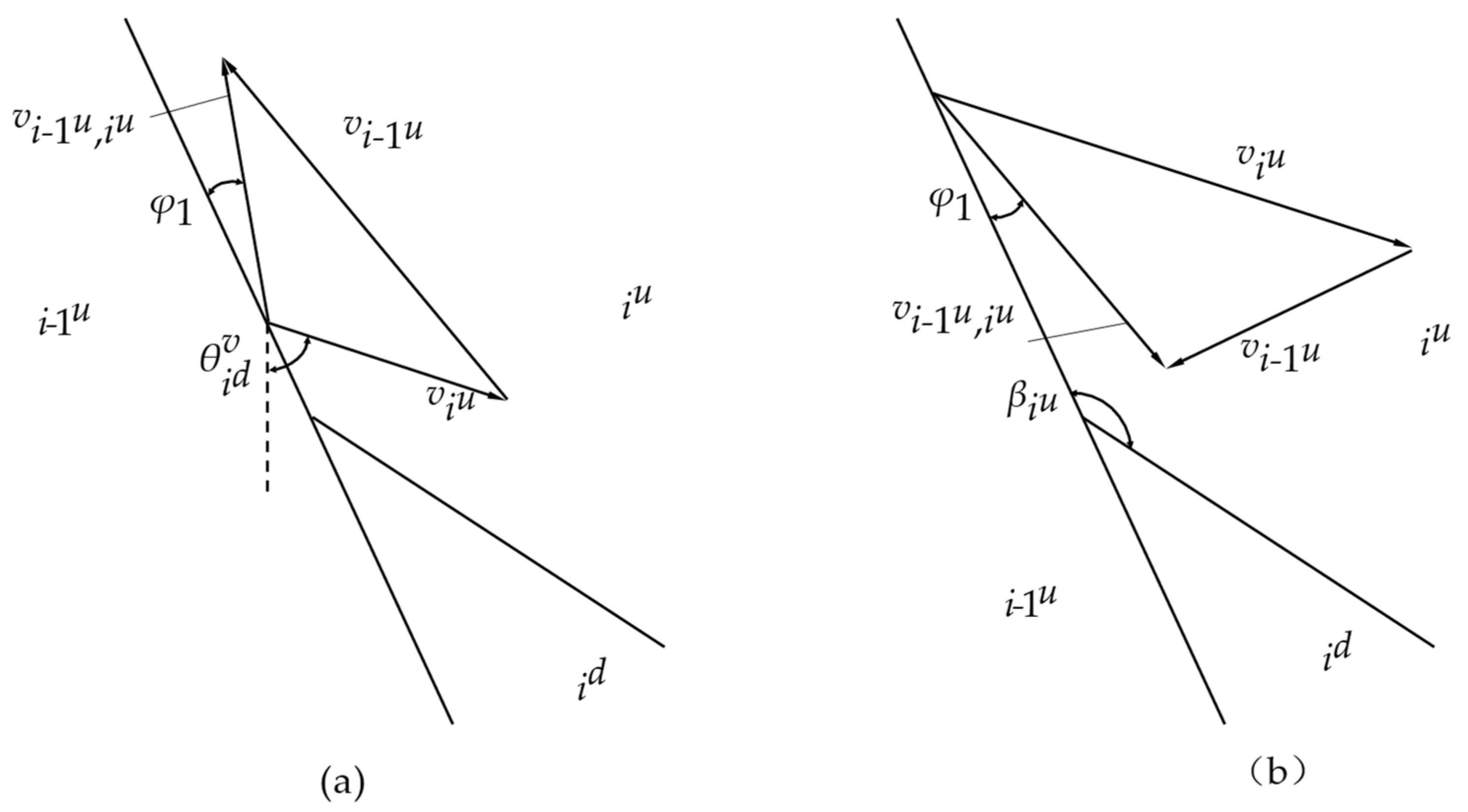
For rigid block iu, since the direction angle of its absolute velocity vector cannot be determined directly, it is necessary to analyze the compatible velocity relationship between rigid block i − 1u and iu, rigid block id and iu, and perform simultaneous solution.
- (1)
Type Ⅲ–ⅰu rigid block and i − 1u rigid block:
The compatible velocity relationship of rigid block
, as shown in
Figure 8:
For
Figure 8a, the relative velocity
between the rigid block
i − 1
u and
iu face upwards along the velocity discontinuity and forms an angle
φ1 Requirements of Equations (22) and (23):
The relative velocity
between the rigid block in
Figure 8b face downward along the velocity discontinuity and forms an angle
φ1.
Requirements of Equations (24) and (25):
- (2)
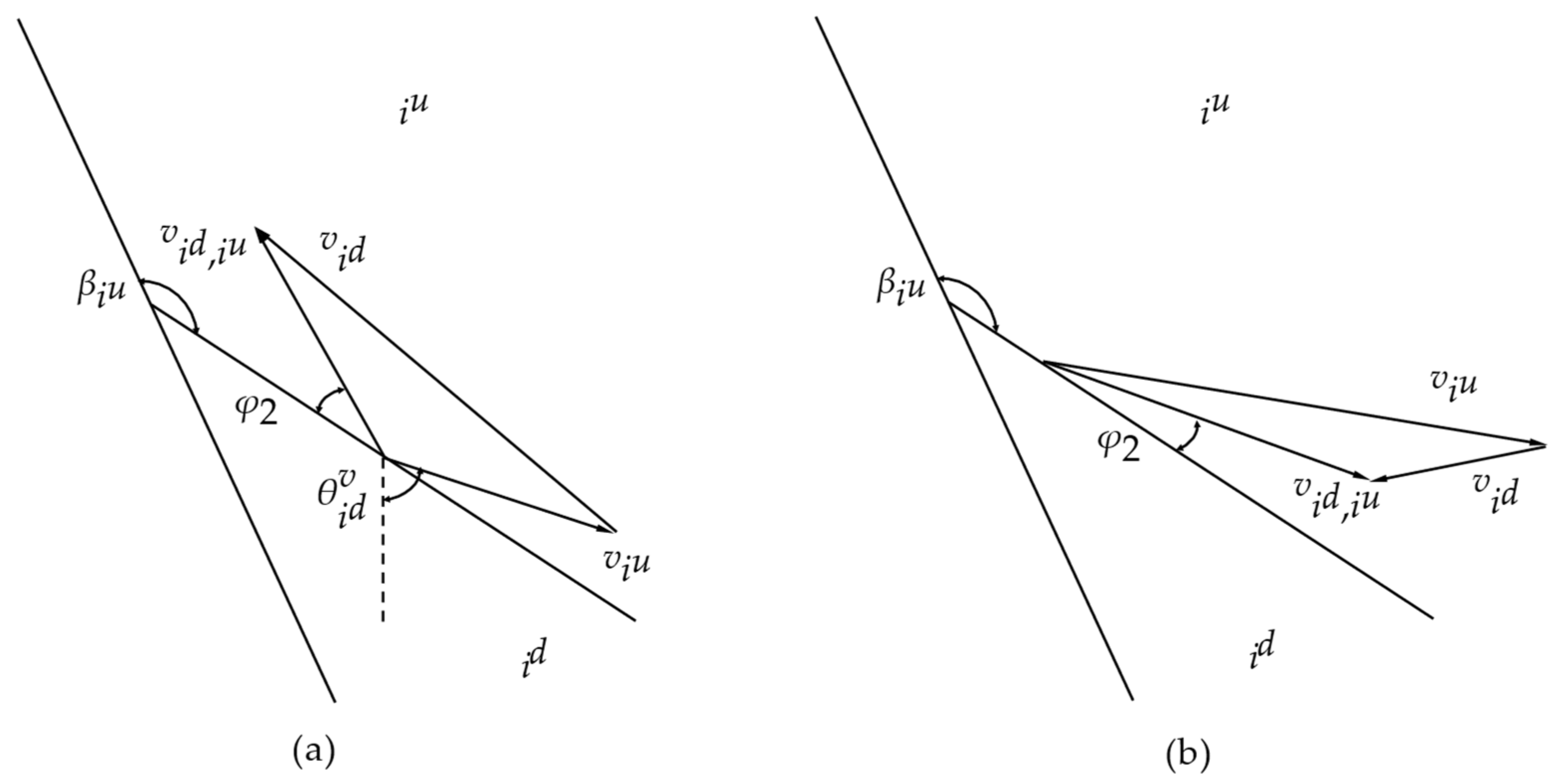
Type III–ⅰu and id:
The possibility of two compatible velocity relationships between rigid block
and
is shown in
Figure 9:
For
Figure 9a, the relative velocity
between the rigid block
id and
iu face upwards along the velocity discontinuity and forms an angle
φ2.
Requirements of Equations (27) and (28):
The relative velocity
between the rigid block in
Figure 9b faces downward along the velocity discontinuity and forms an angle
φ2.
Requirements of Equations (30) and (31):
To solve the velocity vector of rigid block iu, it can be seen from the above that there are four cases (2*2). For example, we can get by Equations (22) and (27) and then get each velocity vector by substituting Equations (22), (23), (27) and (28). The other three cases are also considered similar.
When calculating the velocity vector of Type III rigid blocks, there will be two types of connections in the two–layered strip foundation multi–rigid block failure mechanism. If the rigid block i − 1 is Type II, it is only necessary to replace all rigid blocks i − 1u in the above calculation formula with rigid block i − 1 to calculate normally.
2.3. Upper Limit Solution of Ultimate Bearing Capacity of Two–Layered Foundation
The virtual work theory serves as the foundation for the upper−bound limit analysis theorem. According to the virtual work concept, the elastic−plastic material deforms with a little displacement (virtual displacement). According to Equation (33), under the influence of this virtual displacement, the virtual external power produced by the external force acting on the elastic−plastic material is equal to the virtual internal power produced by the system’s internal virtual strain.
In the multi–rigid block failure mechanism of the two–layered strip foundation, the work performed by the external force includes: the power
made by the ultimate load
Pu of the foundation, the power
made by the overload
q on both sides of the foundation, and the power
made by the gravity of each rigid block. Where
represents gravity work of No.0 rigid block,
and
represent gravity work of rigid block
and
, and
represents gravity work of rigid block
i. The expressions of each external force power are as follows: Equations (35)–(40).
At the connection of different types of rigid blocks, the division of the area of the rigid blocks will be different. It is necessary to recalculate the gravity work of its rigid block i, which is similar to the above expression and will not be introduced in detail.
The soil mass does not experience internal plastic deformation according to the upper bound theory of limit analysis, and the internal force energy consumption only happens on the velocity discontinuities , (including , , , , but excluding , because does not belong to the interface of rigid blocks) between adjacent rigid blocks. The internal force energy consumption expression is shown in Equations (40)–(43).
where
and
refer to the internal force energy consumption on the velocity discontinuity between each rigid block in the failure mechanism, and the subscripts
l and
d correspond to the side lengths
L and
D of the rigid block in the failure mechanism.
At the connection of different types of rigid blocks, such as Type Ⅲ rigid blocks connected to type Ⅱ rigid blocks, the corresponding c1 and φ1 should be used for the calculation of the velocity discontinuity plane in Equation (43). Other calculation methods are the same.
According to the principle of virtual work, in the assumed failure model, the external force power and internal energy consumption are equal, then the expression of ultimate bearing capacity
Pu can be deduced according to Equation (44).


