
Sequential Data Processing for IMERG Satellite Rainfall Comparison and Improvement Using LSTM and ADAM Optimizer
 , , and
Abstract
:1. Introduction
2. Materials and Methods
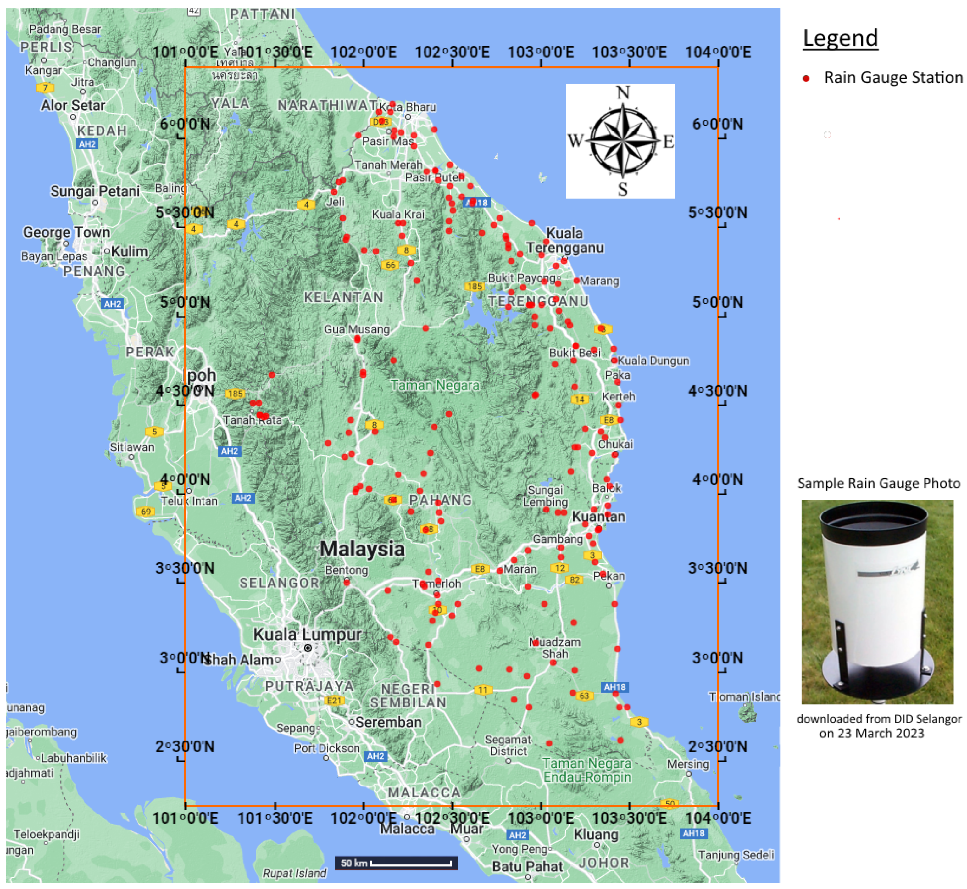
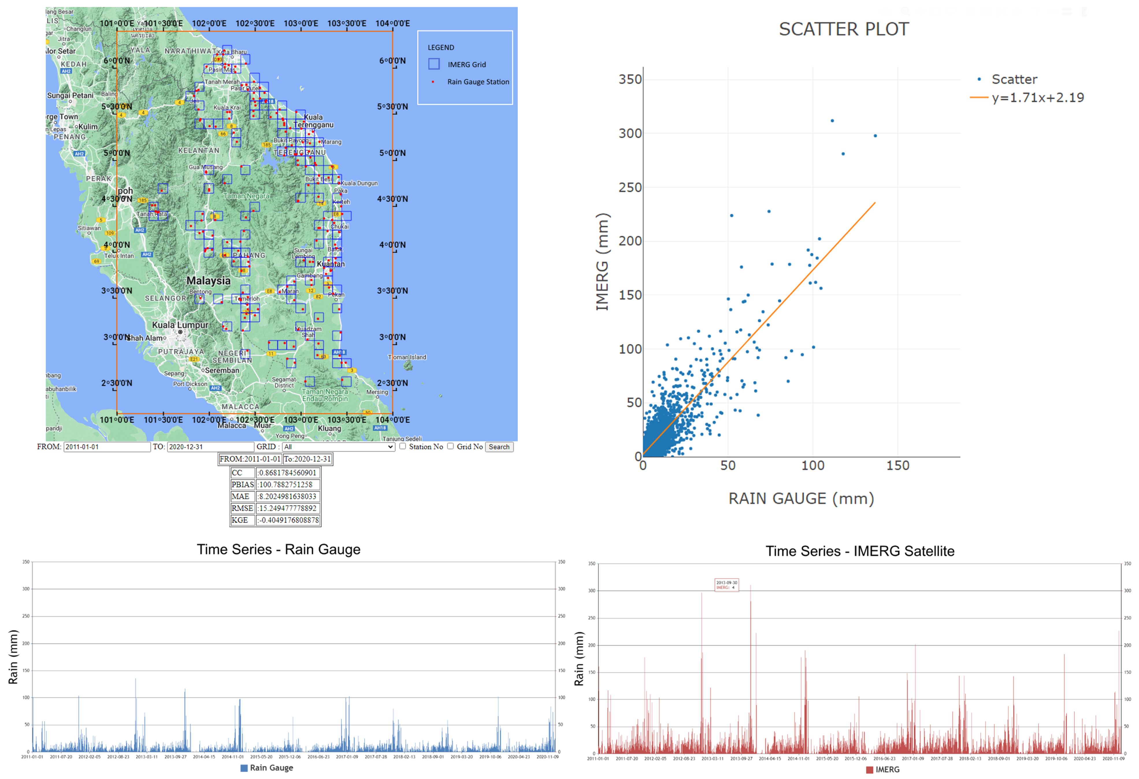
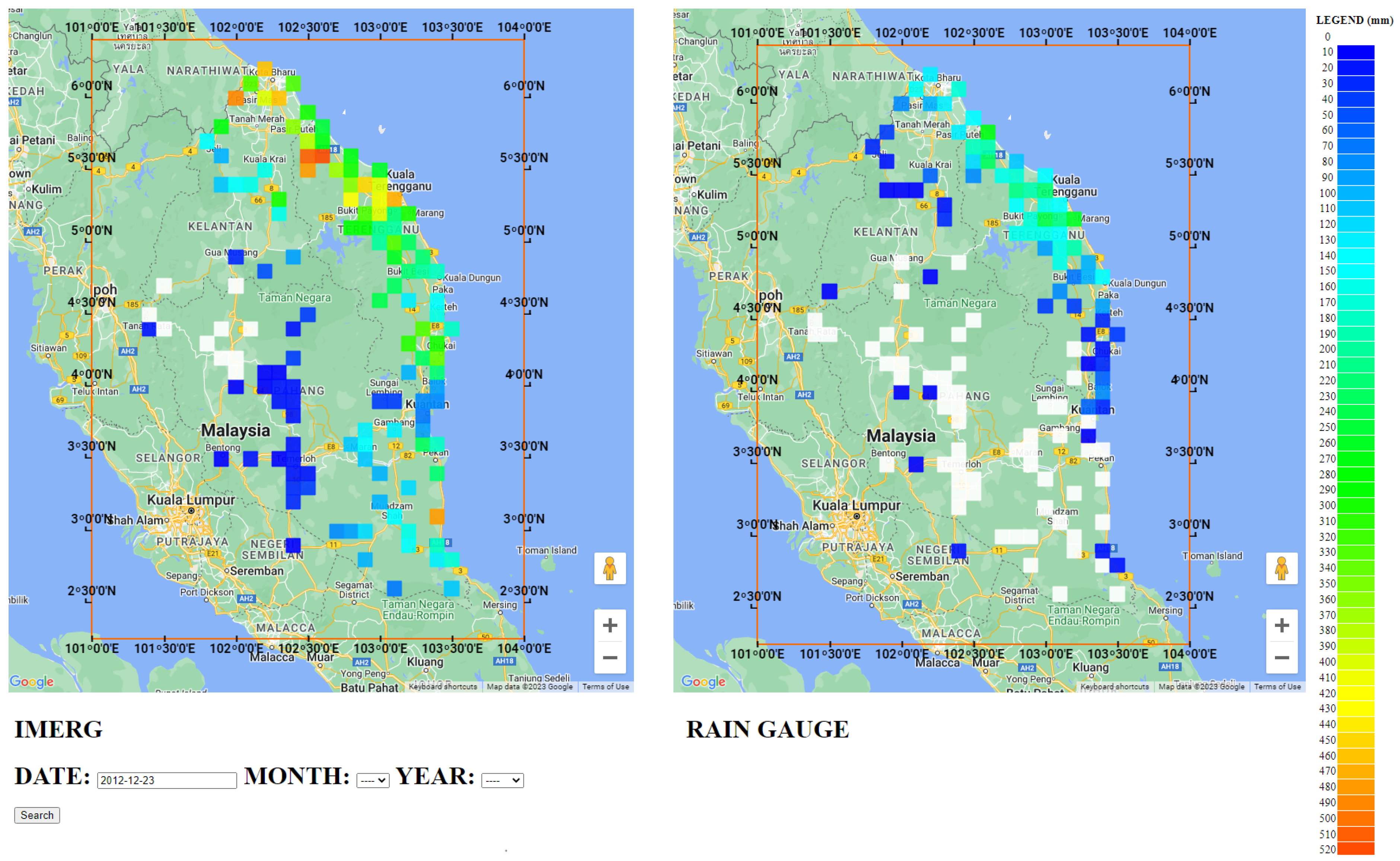
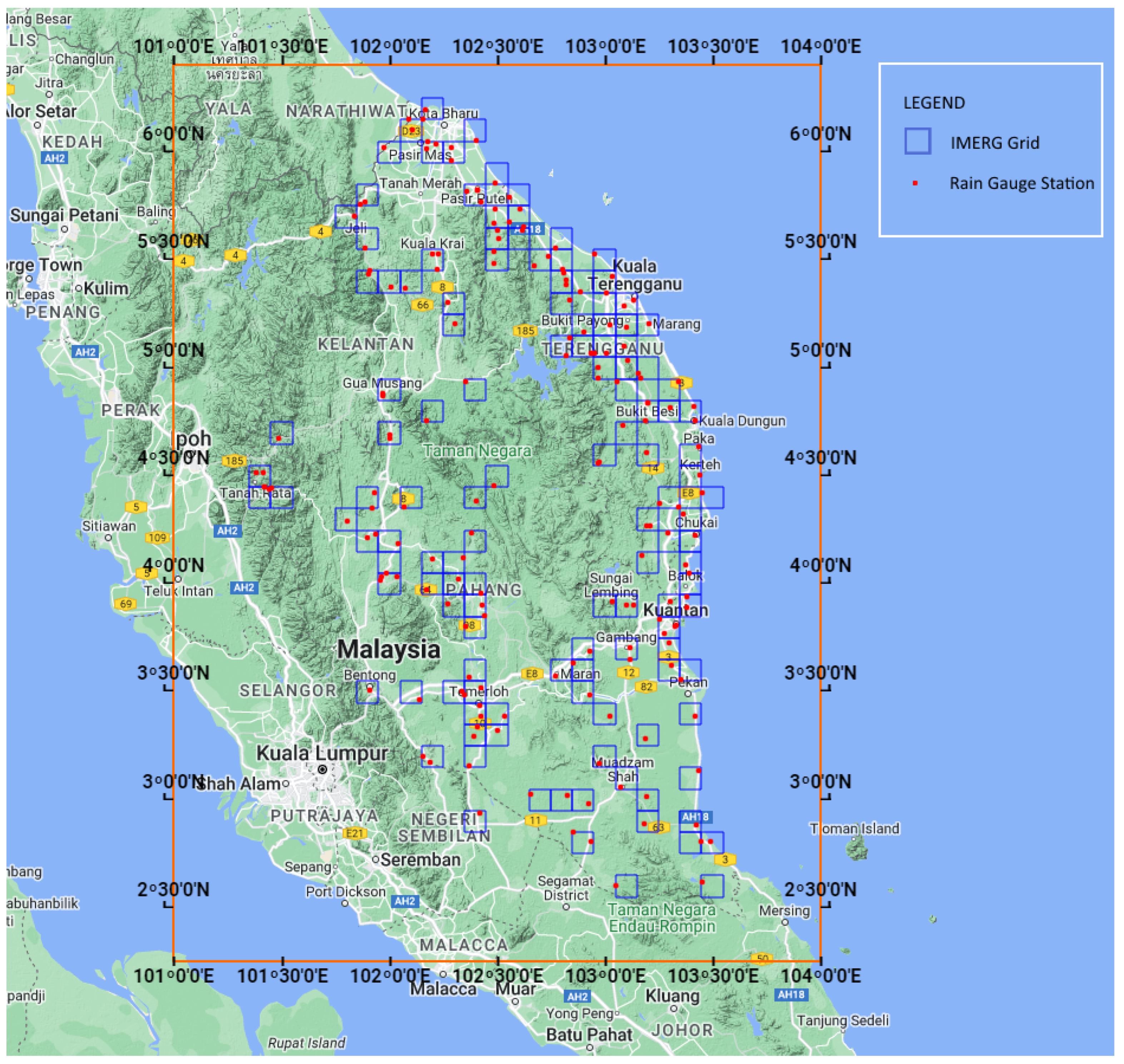
2.1. Study Site
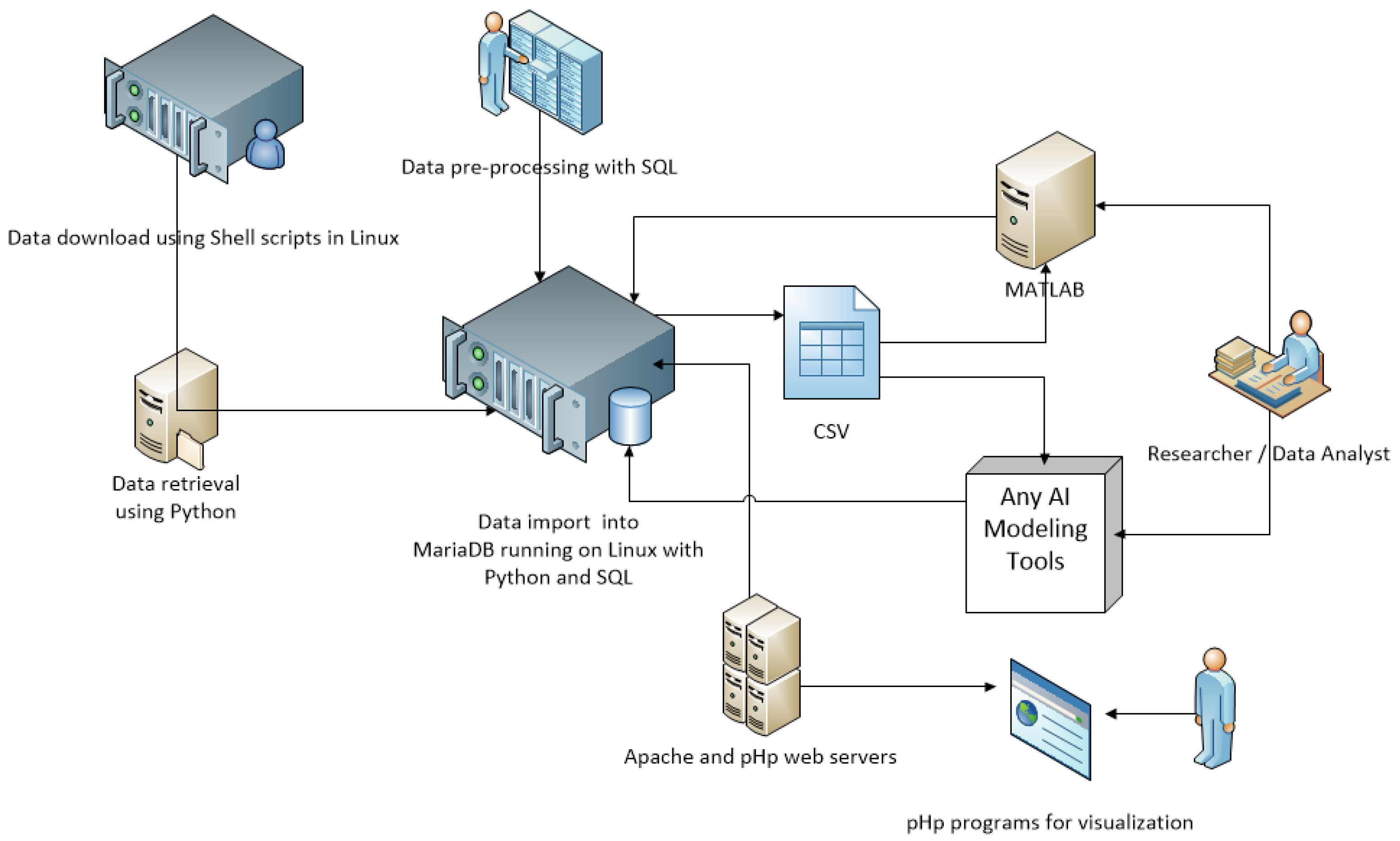
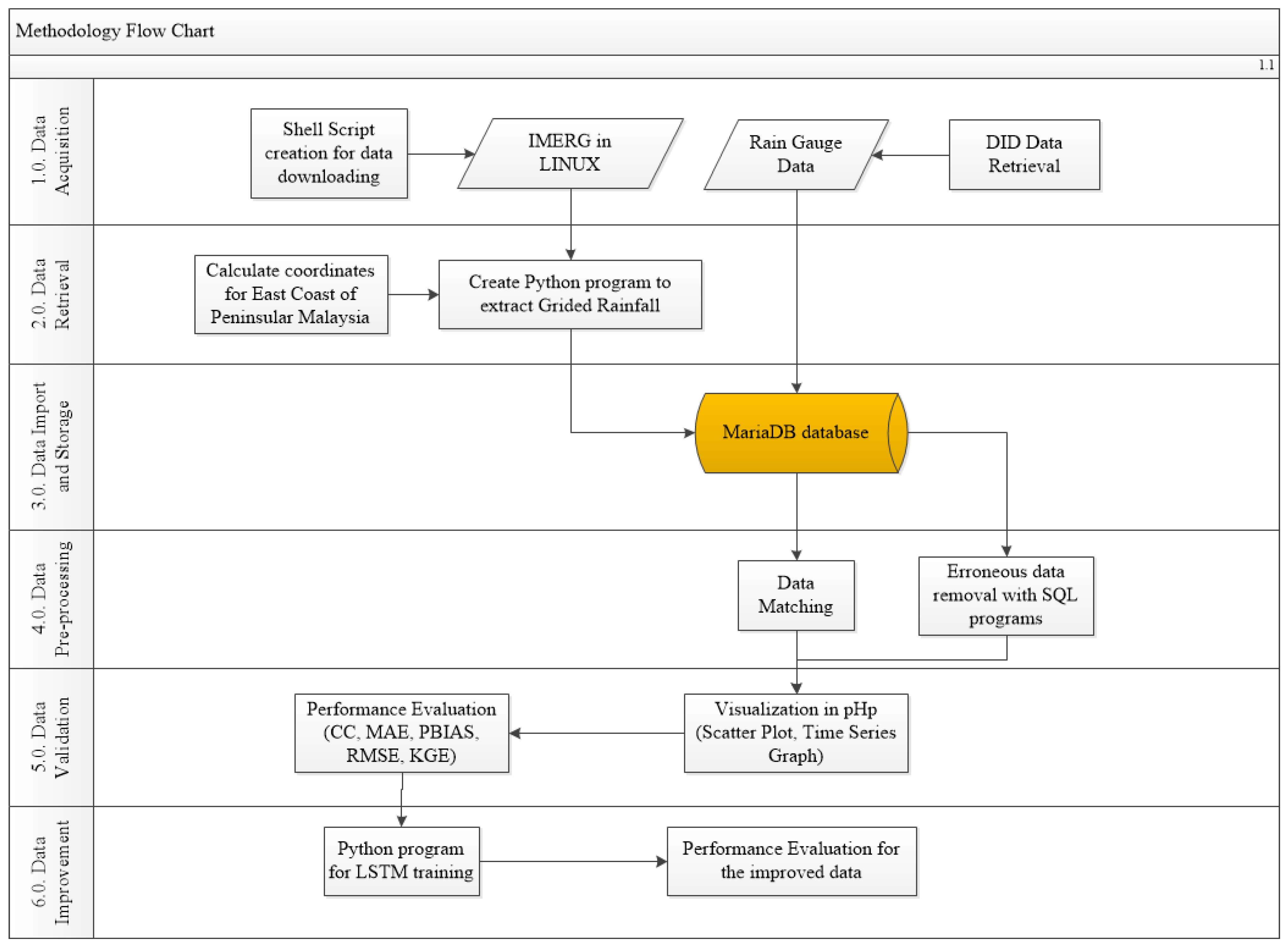
2.2. Methodology
2.2.1. Phase 1: Data Acquisition
2.2.2. Phase 2: Data Retrieval
2.2.3. Phase 3: Data Import and Storage
2.2.4. Phase 4: Data Pre-Processing
2.2.5. Phase 5: Data Validation
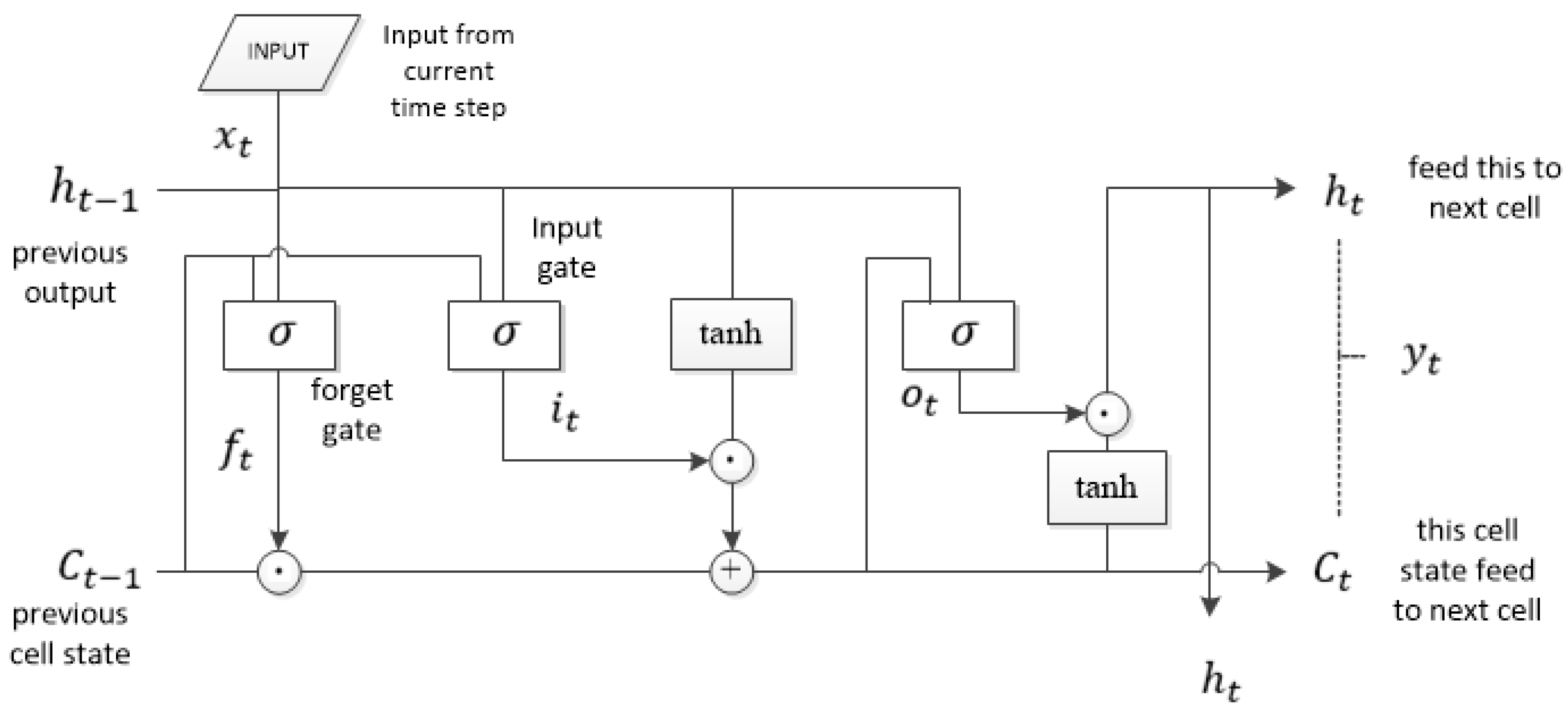
2.2.6. Phase 6: Data Improvement
2.3. Development of pHp Programs
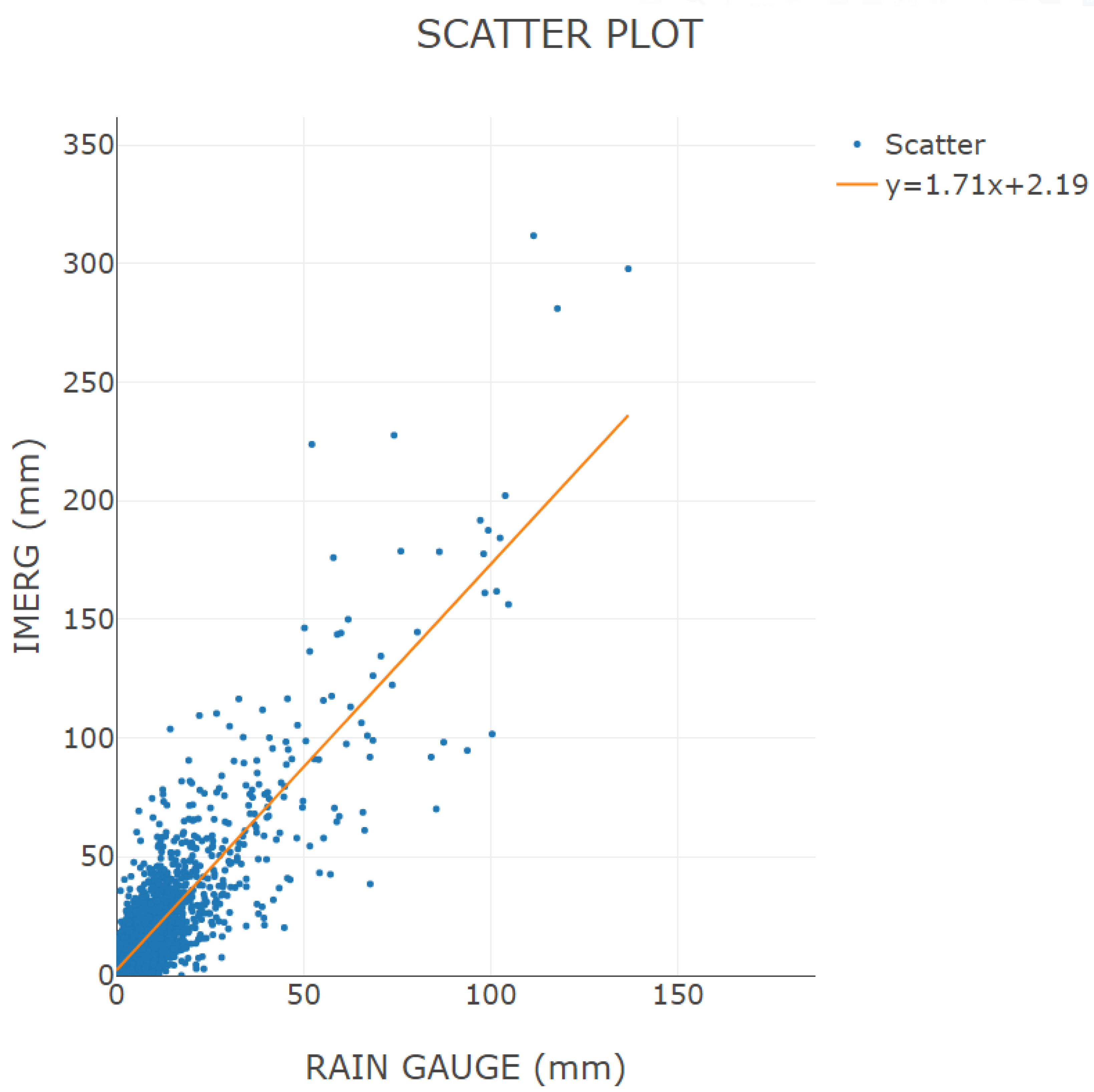
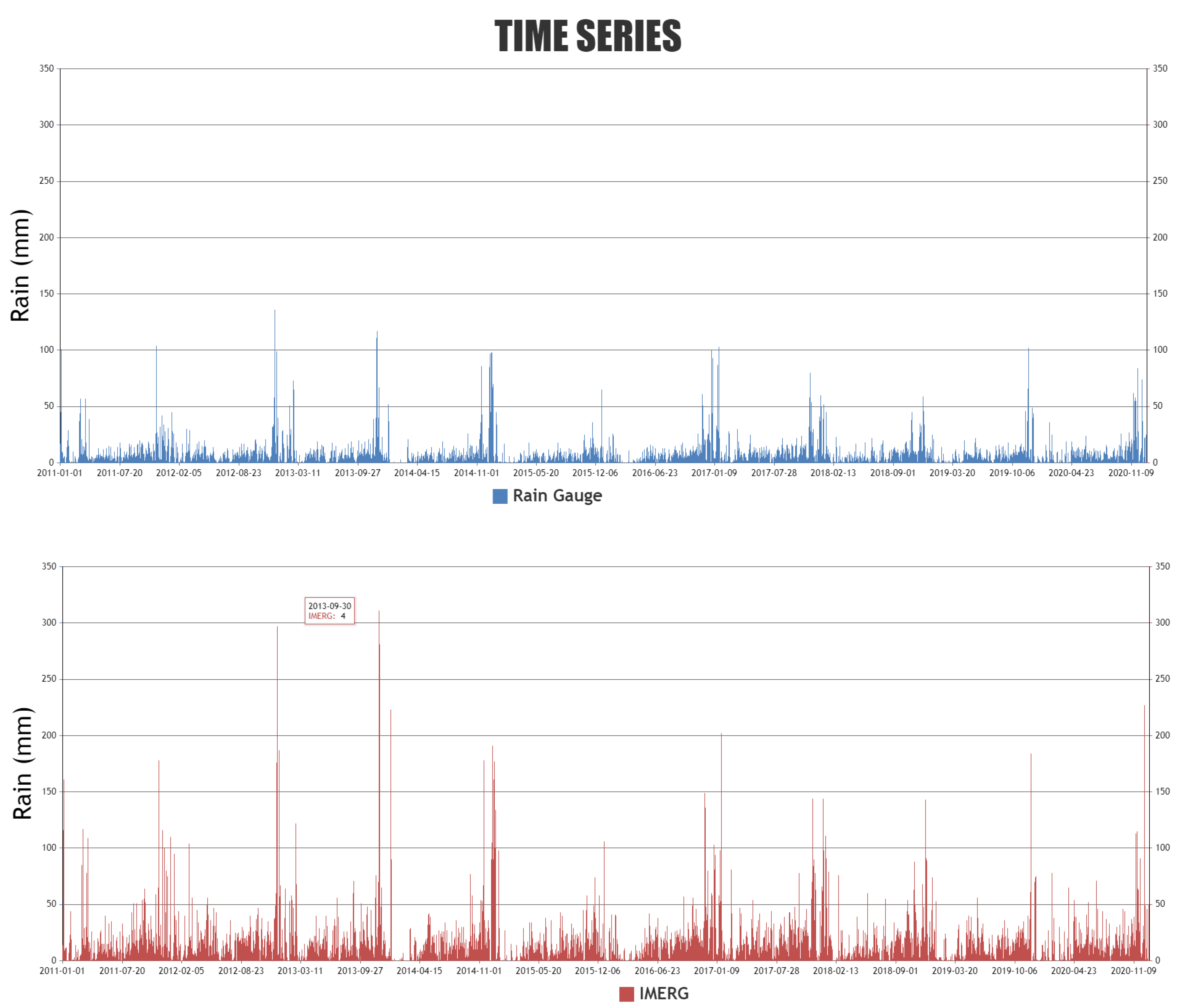
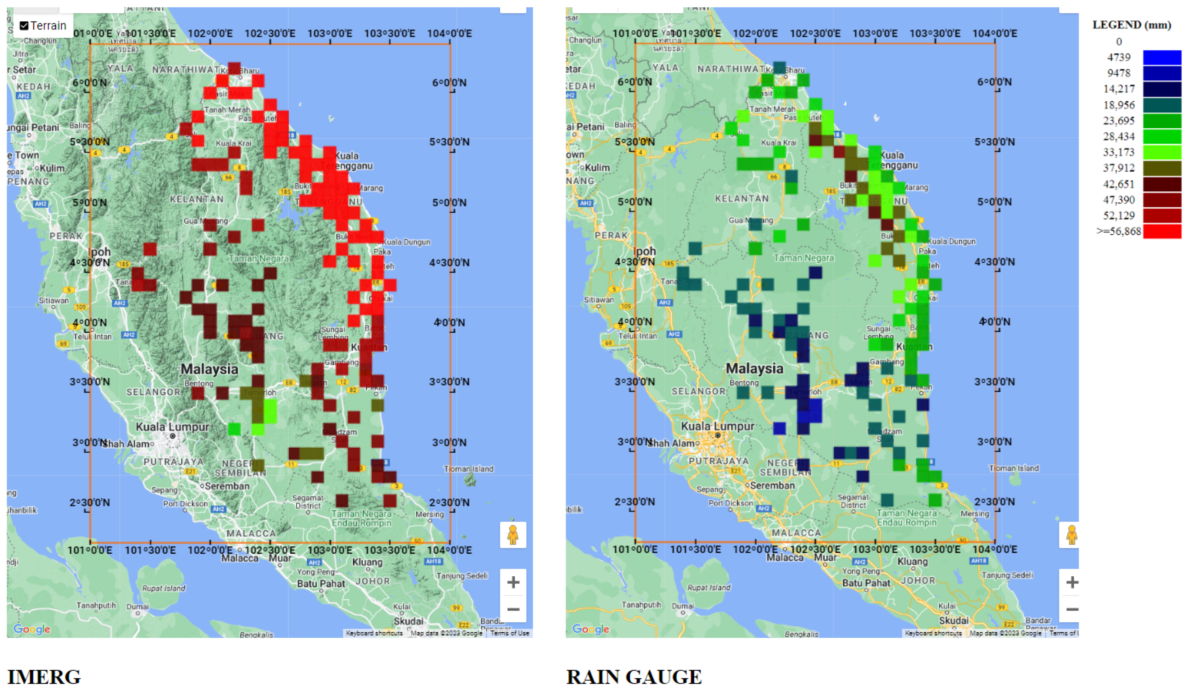
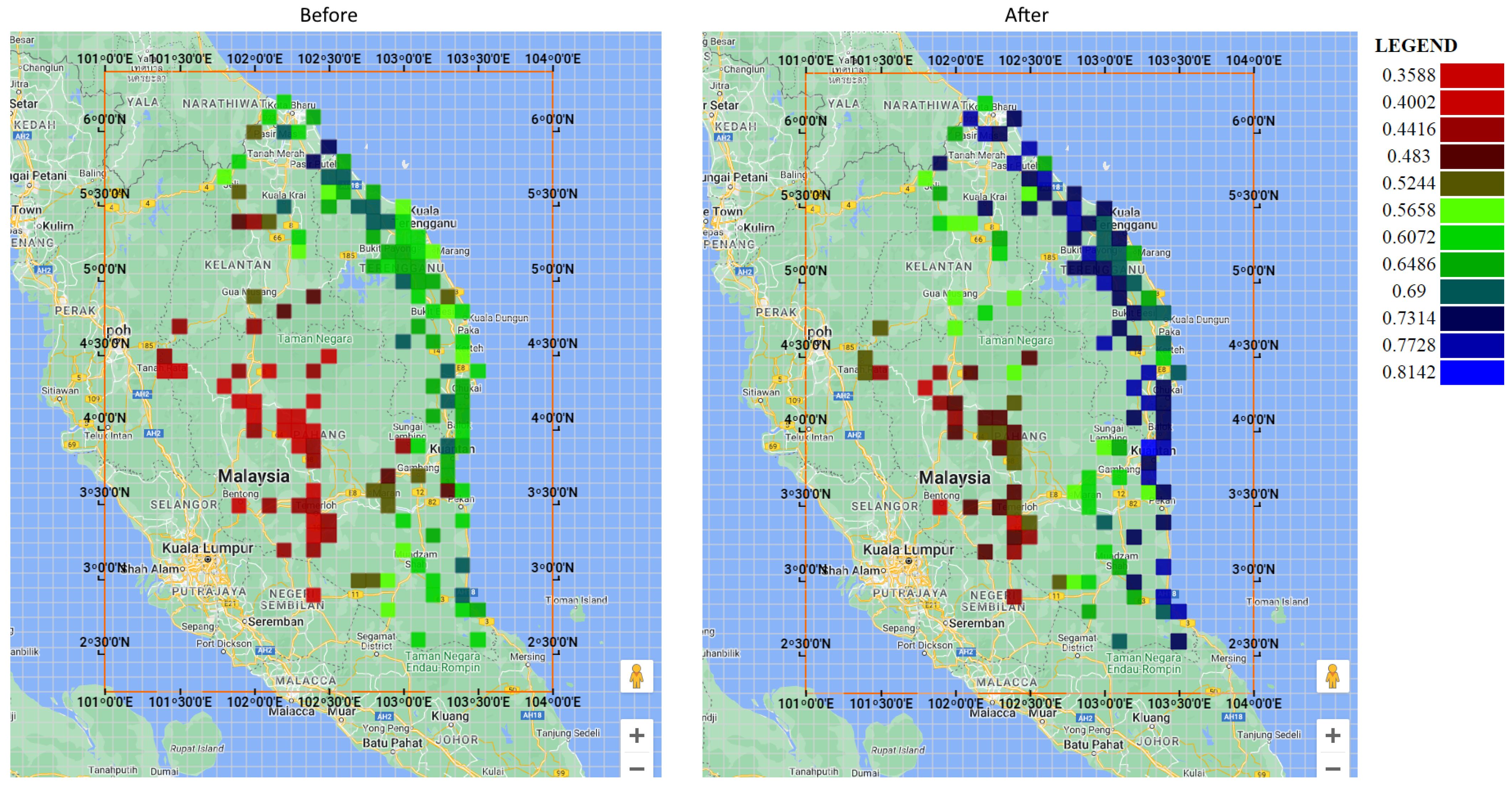
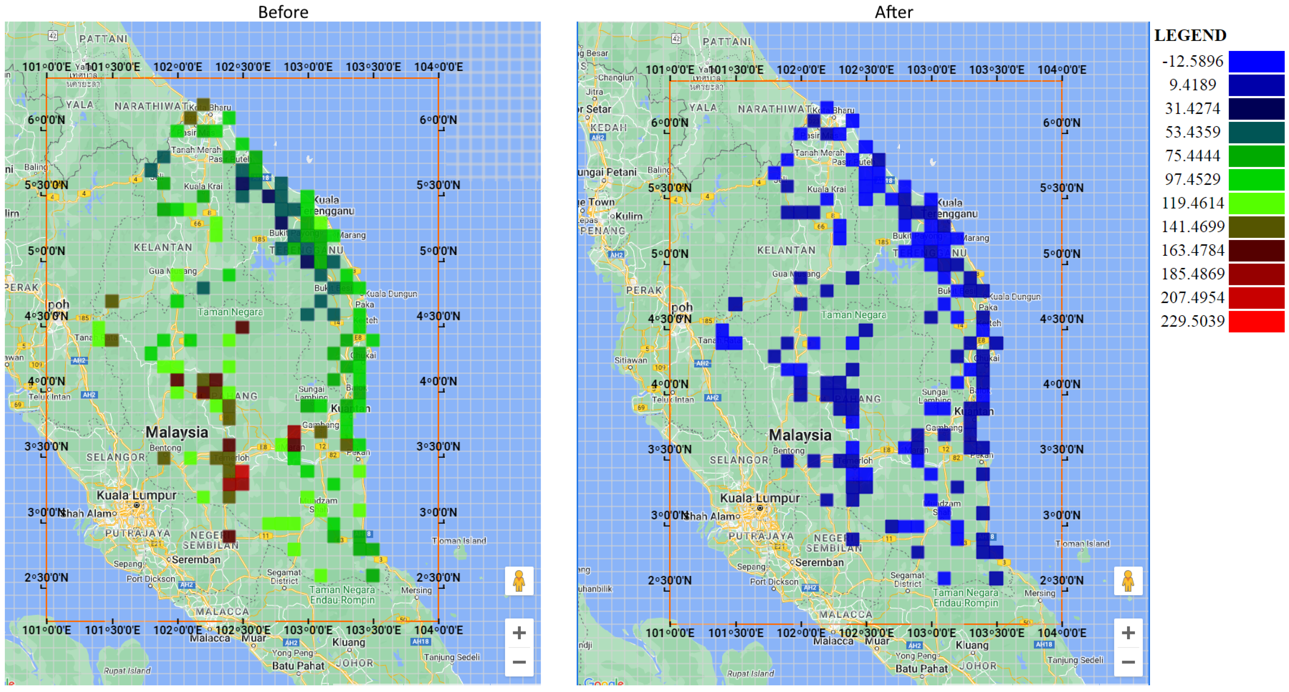
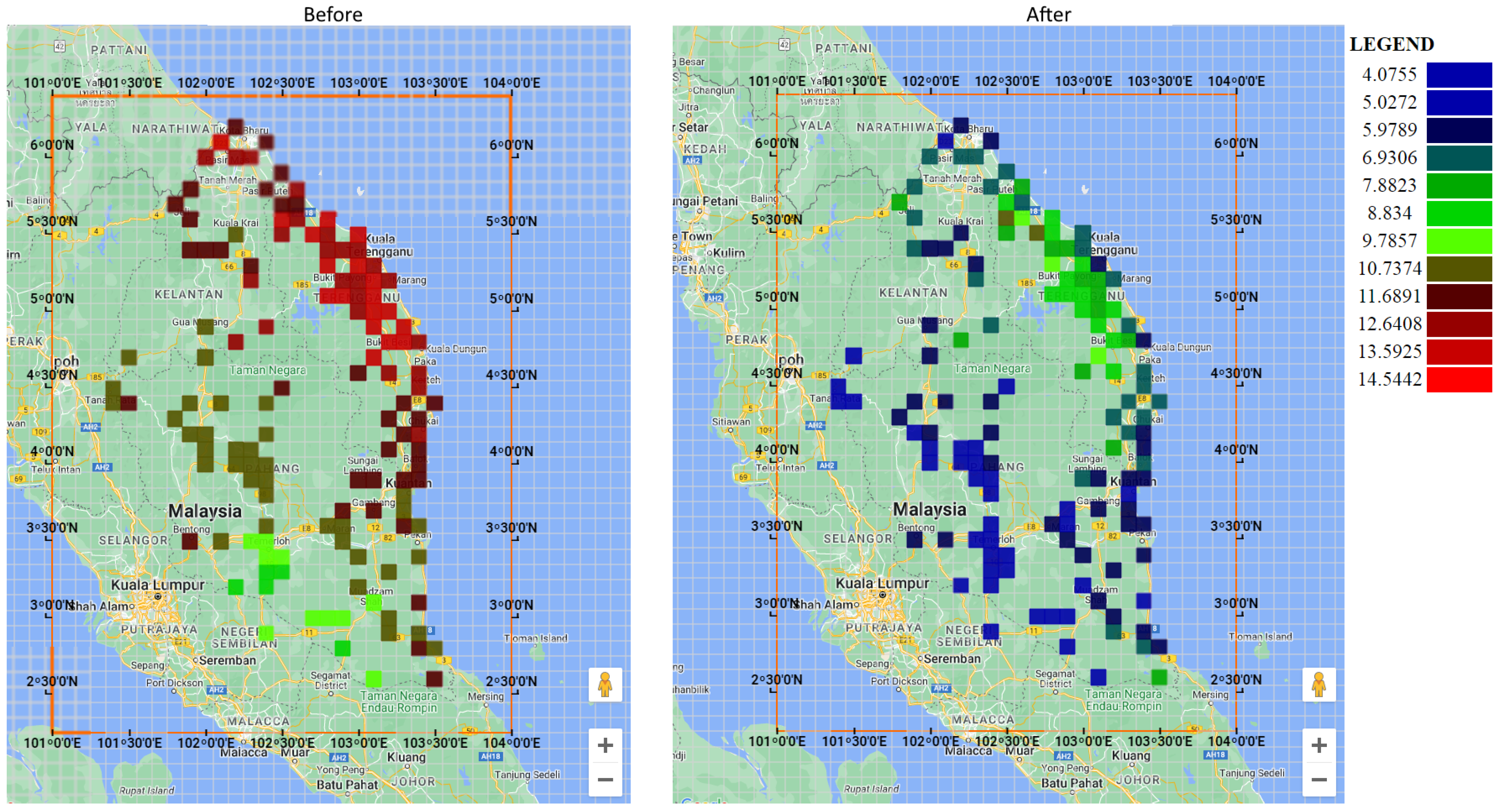
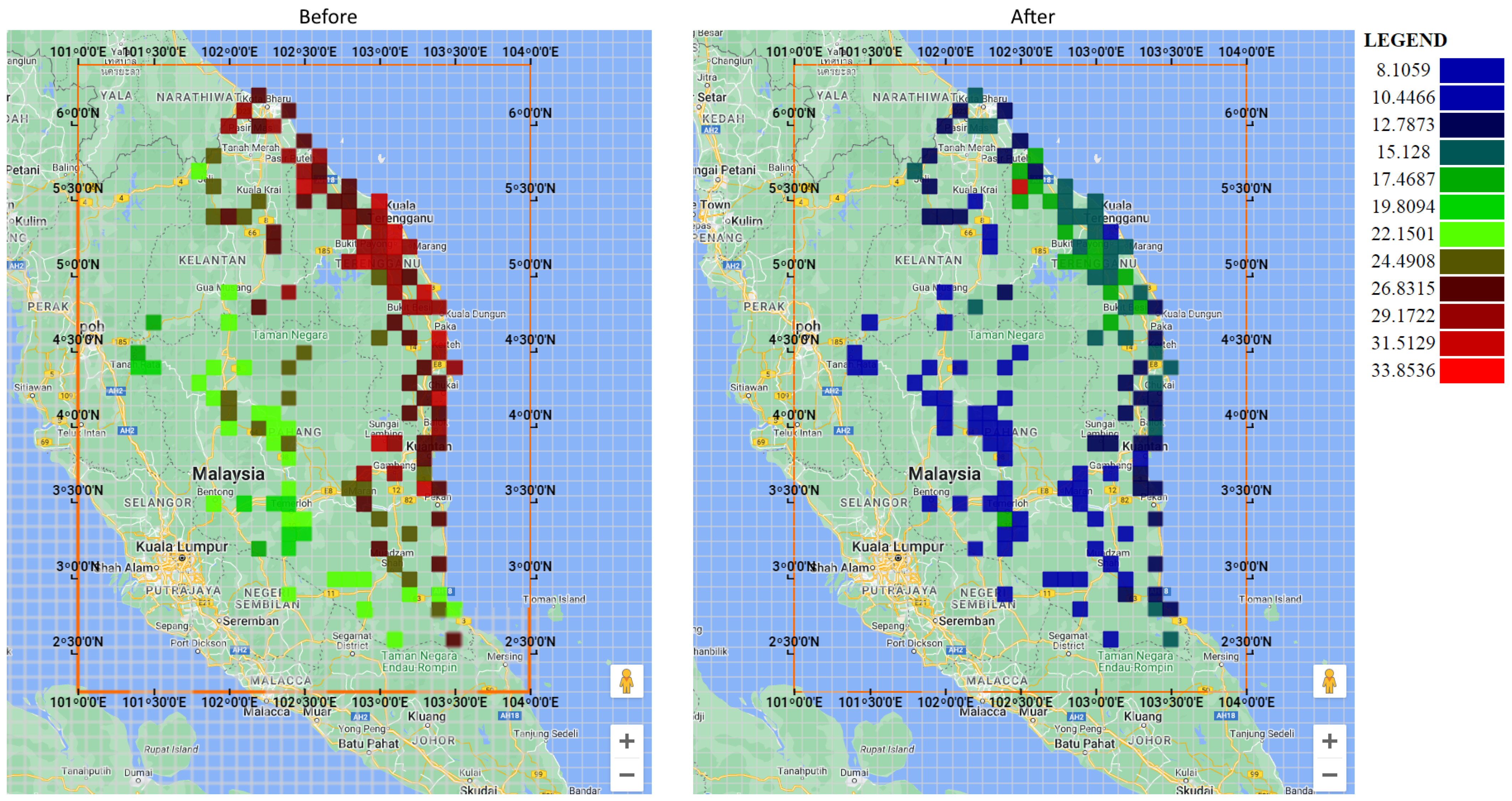
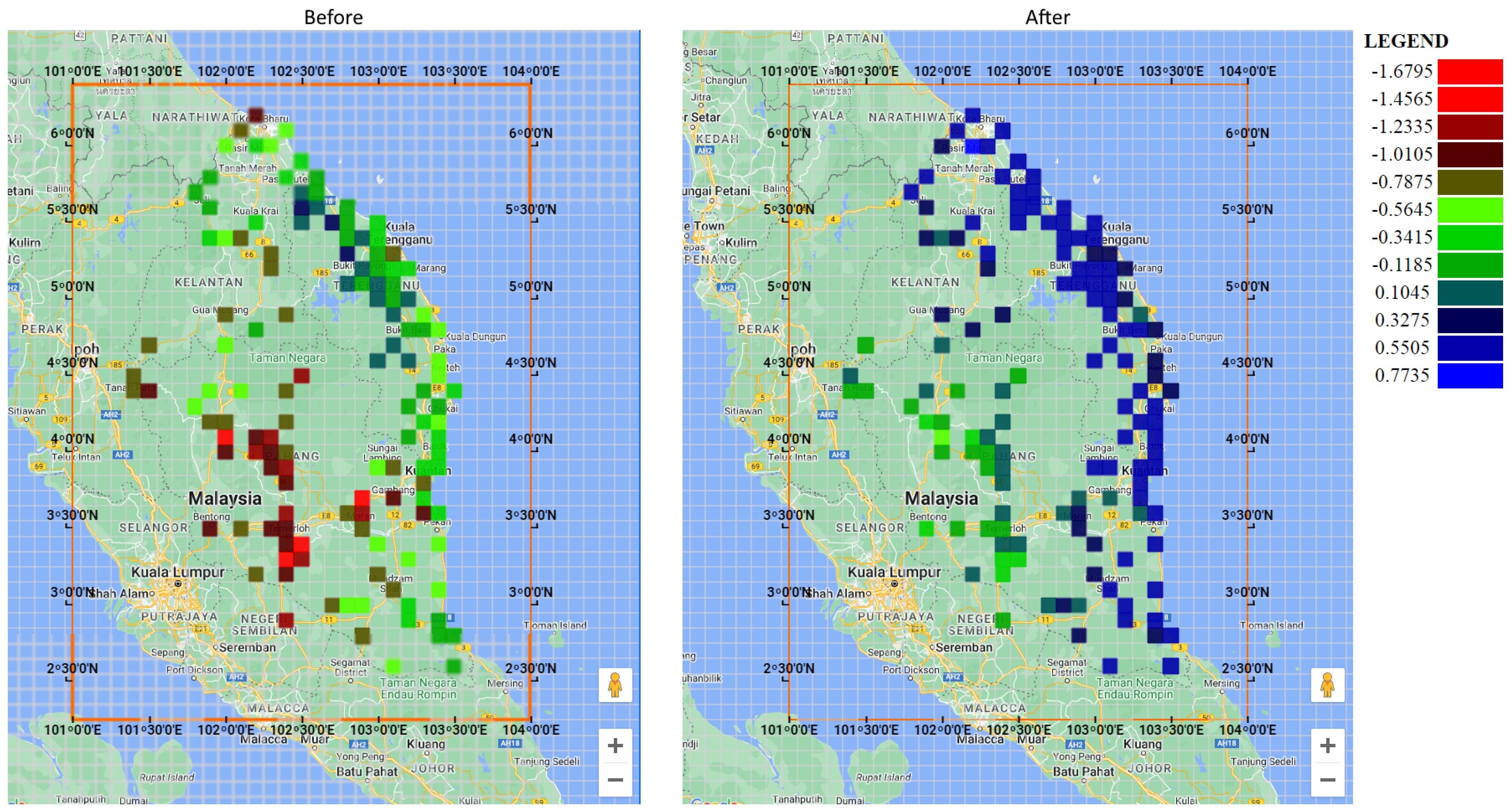
3. Results
4. Discussion
5. Conclusions
Author Contributions
Funding
Institutional Review Board Statement
Informed Consent Statement
Data Availability Statement
Acknowledgments
Conflicts of Interest
Abbreviations
| IMERG | Integrated Multi-Satellite Retrievals for GPM |
| LSTM | Long Short-Term Memory |
| ADAM | Adaptive Moment Estimation |
| MAE | Mean Square Error |
| RMSE | Root-Mean-Square Error |
| KGE | Kling–Gupta Efficiency |
| SQL | Structured Query Language |
| pHp | Hypertext Pre-processor |
| ML | Machine Learning |
| DL | Deep Learning |
| SPE | Satellite Precipitation Estimation |
| RNN | Recurrent Neural Network |
| CSV | Comma Separated Values |
| DID | Department of Irrigation and Drainage |
| EXE | Executable |
| HTML | Hypertext Markup Language |
References
- Eltahir, E.A.B.; Bras, R.L. Precipitation recycling. Rev. Geophys. 1996, 34, 367–378. [Google Scholar] [CrossRef]
- Kidd, C. Satellite rainfall climatology: A review. Int. J. Climatol. 2001, 21, 1041–1066. [Google Scholar] [CrossRef]
- Kidd, C.; Becker, A.; Huffman, G.J.; Muller, C.L.; Joe, P.; Skofronick-Jackson, G.; Kirschbaum, D.B. So, How Much of the Earth’s Surface Is Covered by Rain Gauges? Bull. Am. Meteorol. Soc. 2017, 98, 69–78. [Google Scholar] [CrossRef]
- Ma, Q.; Li, Y.; Feng, H.; Yu, Q.; Zou, Y.; Liu, F.; Pulatov, B. Performance evaluation and correction of precipitation data using the 20-year IMERG and TMPA precipitation products in diverse subregions of China. Atmos. Res. 2021, 249, 105304. [Google Scholar] [CrossRef]
- Jiang, S.; Ren, L.; Hong, Y.; Yong, B.; Yang, X.; Yuan, F.; Ma, M. Comprehensive evaluation of multi-satellite precipitation products with a dense rain gauge network and optimally merging their simulated hydrological flows using the Bayesian model averaging method. J. Hydrol. 2012, 452–453, 213–225. [Google Scholar] [CrossRef]
- Gebremicael, T.G.; Mohamed, Y.A.; Zaag, P.v.; Berhe, A.G.; Haile, G.G.; Hagos, E.Y.; Hagos, M.K. Comparison and validation of eight satellite rainfall products over the rugged topography of Tekeze-Atbara Basin at different spatial and temporal scales. Hydrol. Earth Syst. Sci. Discuss. 2017, 2017, 1–31. [Google Scholar]
- Turini, N.; Thies, B.; Bendix, J. Estimating High Spatio-Temporal Resolution Rainfall from MSG1 and GPM IMERG Based on Machine Learning: Case Study of Iran. Remote Sens. 2019, 11, 2307. [Google Scholar] [CrossRef] [Green Version]
- Hong, Y.; Zhang, Y.; Khan, S. Hydrologic Remote Sensing: Capacity Building for Sustainability and Resilience; CRC Press: Boca Raton, FL, USA, 2016. [Google Scholar]
- Llauca, H.; Lavado-Casimiro, W.; León, K.; Jimenez, J.; Traverso, K.; Rau, P. Assessing Near Real-Time Satellite Precipitation Products for Flood Simulations at Sub-Daily Scales in a Sparsely Gauged Watershed in Peruvian Andes. Remote Sens. 2021, 13, 826. [Google Scholar] [CrossRef]
- Kim, T.; Yang, T.; Zhang, L.; Hong, Y. Near real-time hurricane rainfall forecasting using convolutional neural network models with Integrated Multi-satellitE Retrievals for GPM (IMERG) product. Atmos. Res. 2022, 270, 106037. [Google Scholar] [CrossRef]
- Liu, C.-Y.; Aryastana, P.; Liu, G.-R.; Huang, W.-R. Assessment of satellite precipitation product estimates over Bali Island. Atmos. Res. 2020, 244, 105032. [Google Scholar] [CrossRef]
- Huffman, G.J.; Bolvin, D.T.; Nelkin, E.J.; Wolff, D.B.; Adler, R.F.; Gu, G.; Hong, Y.; Bowman, K.P.; Stocker, E.F. The TRMM multisatellite precipitation analysis (TMPA): Quasi-global, multiyear, combined-sensor precipitation estimates at fine scales. J. Hydrometeorol. 2007, 8, 38–55. [Google Scholar] [CrossRef]
- Joyce, R.J.; Janowiak, J.E.; Arkin, P.A.; Xie, P. CMORPH: A method that produces global precipitation estimates from passive microwave and infrared data at high spatial and temporal resolution. J. Hydrometeorol. 2004, 5, 487–503. [Google Scholar] [CrossRef]
- Hsu, K.-l.; Gao, X.; Sorooshian, S.; Gupta, H.V. Precipitation estimation from remotely sensed information using artificial neural networks. J. Appl. Meteorol. 1997, 36, 1176–1190. [Google Scholar] [CrossRef]
- Sorooshian, S.; Hsu, K.-L.; Gao, X.; Gupta, H.V.; Imam, B.; Braithwaite, D. Evaluation of PERSIANN system satellite-based estimates of tropical rainfall. Bull. Am. Meteorol. Soc. 2000, 81, 2035–2046. [Google Scholar] [CrossRef]
- Kubota, T.; Shige, S.; Hashizume, H.; Aonashi, K.; Takahashi, N.; Seto, S.; Hirose, M.; Takayabu, Y.N.; Ushio, T.; Nakagawa, K. Global precipitation map using satellite-borne microwave radiometers by the GSMaP project: Production and validation. IEEE Trans. Geosci. Remote Sens. 2007, 45, 2259–2275. [Google Scholar] [CrossRef]
- Funk, C.; Peterson, P.; Landsfeld, M.; Pedreros, D.; Verdin, J.; Shukla, S.; Husak, G.; Rowland, J.; Harrison, L.; Hoell, A. The climate hazards infrared precipitation with stations—A new environmental record for monitoring extremes. Sci. Data 2015, 2, 1–21. [Google Scholar] [CrossRef] [PubMed] [Green Version]
- Huffman, G.J.; Bolvin, D.T.; Braithwaite, D.; Hsu, K.-L.; Joyce, R.J.; Kidd, C.; Nelkin, E.J.; Sorooshian, S.; Stocker, E.F.; Tan, J. Integrated multi-satellite retrievals for the global precipitation measurement (GPM) mission (IMERG). In Satellite Precipitation Measurement; Springer: Cham, Switzerland, 2020; pp. 343–353. [Google Scholar]
- Ma, Y.; Sun, X.; Chen, H.; Hong, Y.; Zhang, Y. A two-stage blending approach for merging multiple satellite precipitation estimates and rain gauge observations: An experiment in the northeastern Tibetan Plateau. Hydrol. Earth Syst. Sci. 2021, 25, 359–374. [Google Scholar] [CrossRef]
- Arshad, M.; Ma, X.; Yin, J.; Ullah, W.; Ali, G.; Ullah, S.; Liu, M.; Shahzaman, M.; Ullah, I. Evaluation of GPM-IMERG and TRMM-3B42 precipitation products over Pakistan. Atmos. Res. 2021, 249, 105341. [Google Scholar] [CrossRef]
- Moazami, S.; Najafi, M.R. A comprehensive evaluation of GPM-IMERG V06 and MRMS with hourly ground-based precipitation observations across Canada. J. Hydrol. 2021, 594, 125929. [Google Scholar] [CrossRef]
- Mekonnen, K.; Melesse, A.M.; Woldesenbet, T.A. Spatial evaluation of satellite-retrieved extreme rainfall rates in the Upper Awash River Basin, Ethiopia. Atmos. Res. 2021, 249, 105297. [Google Scholar] [CrossRef]
- Huang, W.-R.; Liu, P.-Y.; Hsu, J.; Li, X.; Deng, L. Assessment of Near-Real-Time Satellite Precipitation Products from GSMaP in Monitoring Rainfall Variations over Taiwan. Remote Sens. 2021, 13, 202. [Google Scholar] [CrossRef]
- Gan, F.; Gao, Y.; Xiao, L. Comprehensive validation of the latest IMERG V06 precipitation estimates over a basin coupled with coastal locations, tropical climate and hill-karst combined landform. Atmos. Res. 2021, 249, 105293. [Google Scholar] [CrossRef]
- Nepal, B.; Shrestha, D.; Sharma, S.; Shrestha, M.S.; Aryal, D.; Shrestha, N. Assessment of GPM-Era Satellite Products’ (IMERG and GSMaP) Ability to Detect Precipitation Extremes over Mountainous Country Nepal. Atmosphere 2021, 12, 254. [Google Scholar] [CrossRef]
- Palpanas, T. Data Series Management: The Road to Big Sequence Analytics. SIGMOD Rec. 2015, 44, 47–52. [Google Scholar] [CrossRef]
- Huntington, J.L.; Hegewisch, K.C.; Daudert, B.; Morton, C.G.; Abatzoglou, J.T.; McEvoy, D.J.; Erickson, T. Climate Engine: Cloud Computing and Visualization of Climate and Remote Sensing Data for Advanced Natural Resource Monitoring and Process Understanding. Bull. Am. Meteorol. Soc. 2017, 98, 2397–2410. [Google Scholar] [CrossRef]
- Yin, J.; Guo, S.; Gu, L.; Zeng, Z.; Liu, D.; Chen, J.; Shen, Y.; Xu, C.-Y. Blending multi-satellite, atmospheric reanalysis and gauge precipitation products to facilitate hydrological modelling. J. Hydrol. 2021, 593, 125878. [Google Scholar] [CrossRef]
- Amani, M.; Ghorbanian, A.; Ahmadi, S.A.; Kakooei, M.; Moghimi, A.; Mirmazloumi, S.M.; Moghaddam, S.H.A.; Mahdavi, S.; Ghahremanloo, M.; Parsian, S.; et al. Google Earth Engine Cloud Computing Platform for Remote Sensing Big Data Applications: A Comprehensive Review. IEEE J. Sel. Top. Appl. Earth Obs. Remote Sens. 2020, 13, 5326–5350. [Google Scholar] [CrossRef]
- Chen, H.; Chandrasekar, V.; Cifelli, R.; Xie, P. A Machine Learning System for Precipitation Estimation Using Satellite and Ground Radar Network Observations. IEEE Trans. Geosci. Remote Sens. 2020, 58, 982–994. [Google Scholar] [CrossRef]
- Zhang, L.; Li, X.; Zheng, D.; Zhang, K.; Ma, Q.; Zhao, Y.; Ge, Y. Merging multiple satellite-based precipitation products and gauge observations using a novel double machine learning approach. J. Hydrol. 2021, 594, 125969. [Google Scholar] [CrossRef]
- Sadeghi, M.; Nguyen, P.; Hsu, K.; Sorooshian, S. Improving near real-time precipitation estimation using a U-Net convolutional neural network and geographical information. Environ. Model. Softw. 2020, 134, 104856. [Google Scholar] [CrossRef]
- Kühnlein, M.; Appelhans, T.; Thies, B.; Nauss, T. Improving the accuracy of rainfall rates from optical satellite sensors with machine learning—A random forests-based approach applied to MSG SEVIRI. Remote Sens. Environ. 2014, 141, 129–143. [Google Scholar] [CrossRef] [Green Version]
- Srivastava, S. and Lessmann, S. A comparative study of LSTM neural networks in forecasting day-ahead global horizontal irradiance with satellite data. Sol. Energy 2018, 162, 232–247. [Google Scholar] [CrossRef]
- Graves, A.; Jaitly, N.; Mohamed, A.R. Hybrid speech recognition with deep bidirectional LSTM. In Proceedings of the 2013 IEEE Workshop on Automatic Speech Recognition and Understanding, Olomouc, Czech Republic, 8–12 December 2013. [Google Scholar]
- Wang, S.; Jiang, J. Learning natural language inference with LSTM. arXiv 2015, arXiv:1512.08849. [Google Scholar]
- Karevan, Z.; Suykens, J.A. Transductive LSTM for time-series prediction: An application to weather forecasting. Neural Netw. 2020, 125, 1–9. [Google Scholar] [CrossRef] [PubMed]
- DiPietro, R.; Hager, G.D. Chapter 21—Deep learning: RNNs and LSTM. In Handbook of Medical Image Computing and Computer Assisted Intervention; Zhou, S.K., Rueckert, D., Fichtinger, G., Eds.; Academic Press: Cambridge, MA, USA, 2020; pp. 503–519. [Google Scholar]
- Sherstinsky, A. Fundamentals of recurrent neural network (RNN) and long short-term memory (LSTM) network. Phys. D Nonlinear Phenom. 2020, 404, 132306. [Google Scholar] [CrossRef] [Green Version]
- Akbari Asanjan, A.; Yang, T.; Hsu, K.; Sorooshian, S.; Lin, J.; Peng, Q. Short-Term Precipitation Forecast Based on the PERSIANN System and LSTM Recurrent Neural Networks. J. Geophys. Res. Atmos. 2018, 123, 12543–12563. [Google Scholar] [CrossRef]
- Miao, Q.; Pan, B.; Wang, H.; Hsu, K.; Sorooshian, S. Improving Monsoon Precipitation Prediction Using Combined Convolutional and Long Short Term Memory Neural Network. Water 2019, 11, 977. [Google Scholar] [CrossRef] [Green Version]
- Wu, H.; Yang, Q.; Liu, J.; Wang, G. A spatiotemporal deep fusion model for merging satellite and gauge precipitation in China. J. Hydrol. 2020, 584, 124664. [Google Scholar] [CrossRef]
- Hochreiter, S.; Schmidhuber, J. Long Short-Term Memory. Neural Comput. 1997, 9, 1735–1780. [Google Scholar] [CrossRef]
- Dehghani, A.; Moazam, H.M.Z.H.; Mortazavizadeh, F.; Ranjbar, V.; Mirzaei, M.; Mortezavi, S.; Ng, J.L.; Dehghani, A. Comparative evaluation of LSTM, CNN, and ConvLSTM for hourly short-term streamflow forecasting using deep learning approaches. Ecol. Inform. 2023, 75, 102119. [Google Scholar] [CrossRef]
- Sharma, O. Deep challenges associated with deep learning. In Proceedings of the 2019 International Conference on Machine Learning, Big Data, Cloud and Parallel Computing (COMITCon), Faridabad, India, 14–16 February 2019. [Google Scholar]
- Gao, W.; Gao, J.; Yang, L.; Wang, M.; Yao, W. A novel modeling strategy of weighted mean temperature in China using RNN and LSTM. Remote Sens. 2021, 13, 3004. [Google Scholar] [CrossRef]
- Gers, F.A.; Schraudolph, N.N.; Schmidhuber, J. Learning precise timing with LSTM recurrent networks. J. Mach. Learn. Res. 2002, 3, 115–143. [Google Scholar]
- Noh, S.-H. Analysis of gradient vanishing of RNNs and performance comparison. Information 2021, 12, 442. [Google Scholar] [CrossRef]
- Mirzaei, M.; Yu, H.; Dehghani, A.; Galavi, H.; Shokri, V.; Karimi, S.M.; Sookhak, M. A novel stacked long short-term memory approach of deep learning for streamflow simulation. Sustainability 2021, 13, 13384. [Google Scholar] [CrossRef]
- Mohsenzadeh Karimi, S.; Mirzaei, M.; Dehghani, A.; Galavi, H.; Huang, Y.F. Hybrids of machine learning techniques and wavelet regression for estimation of daily solar radiation. Stoch. Environ. Res. Risk Assess. 2022, 36, 4255–4269. [Google Scholar] [CrossRef]
- Roh, Y.; Heo, G.; Whang, S.E. A Survey on Data Collection for Machine Learning: A Big Data—AI Integration Perspective. IEEE Trans. Knowl. Data Eng. 2021, 33, 1328–1347. [Google Scholar] [CrossRef] [Green Version]
- Woldemeskel, F.M.; Sivakumar, B.; Sharma, A. Merging gauge and satellite rainfall with specification of associated uncertainty across Australia. J. Hydrol. 2013, 499, 167–176. [Google Scholar] [CrossRef]
- Villalobos-Herrera, R.; Blenkinsop, S.; Guerreiro, S.B.; O’Hara, T.; Fowler, H.J. Sub-hourly resolution quality control of rain-gauge data significantly improves regional sub-daily return level estimates. Q. J. R. Meteorol. Soc. 2022, 148, 3252–3271. [Google Scholar] [CrossRef] [PubMed]
- Hsu, J.; Huang, W.-R.; Liu, P.-Y.; Li, X. Validation of CHIRPS Precipitation Estimates over Taiwan at Multiple Timescales. Remote Sens. 2021, 13, 254. [Google Scholar] [CrossRef]
- Bhuiyan, M.A.E.; Yang, F.; Biswas, N.K.; Rahat, S.H.; Neelam, T.J. Machine learning-based error modeling to improve GPM IMERG precipitation product over the brahmaputra river basin. Forecasting 2020, 2, 248–266. [Google Scholar] [CrossRef]
- Lazri, M.; Labadi, K.; Brucker, J.M.; Ameur, S. Improving satellite rainfall estimation from MSG data in Northern Algeria by using a multi-classifier model based on machine learning. J. Hydrol. 2020, 584, 124705. [Google Scholar] [CrossRef]
- Mayowa, O.O.; Pour, S.H.; Shahid, S.; Mohsenipour, M.; Harun, S.B.; Heryansyah, A.; Ismail, T. Trends in rainfall and rainfall-related extremes in the east coast of peninsular Malaysia. J. Earth Syst. Sci. 2015, 124, 1609–1622. [Google Scholar] [CrossRef] [Green Version]
- Juneng, L.; Tangang, F.; Reason, C. Numerical case study of an extreme rainfall event during 9–11 December 2004 over the east coast of Peninsular Malaysia. Meteorol. Atmos. Phys. 2007, 98, 81–98. [Google Scholar] [CrossRef]
- Hai, O.S.; Samah, A.A.; Chenoli, S.N.; Subramaniam, K.; Mazuki, M.Y.A. Extreme rainstorms that caused devastating flooding across the east coast of Peninsular Malaysia during November and December 2014. Weather. Forecast. 2017, 32, 849–872. [Google Scholar] [CrossRef]
- Svennerberg, G. Beginning Google Maps API 3; Apress: New York, NY, USA, 2010. [Google Scholar]
- Hu, L.; He, Z.; Liu, J.; Zheng, C. Method for Measuring the Information Content of Terrain from Digital Elevation Models. Entropy 2015, 17, 7021–7051. [Google Scholar] [CrossRef] [Green Version]
- Collette, A. Python and HDF5: Unlocking Scientific Data; O’Reilly Media, Inc.: Sebastopol, CA, USA, 2013. [Google Scholar]
- Van Rossum, G.; Drake, F. Python 3 Reference Manual Createspace; CreateSpace: Scotts Valley, CA, USA, 2009. [Google Scholar]
- Witham, M.; Bender, I.; Gomes, R. Comparative Analysis of MariaDB’s Performance Efficiency as a Suitable Replacement for MySQL. In Proceedings of the 2019 Midwest Instruction and Computing Symposiu, Fargo, ND, USA, 5–6 April 2019. [Google Scholar]
- Lindstrom, J.; Das, D.; Mathiasen, T.; Arteaga, D.; Talagala, N. NVM aware MariaDB database system. In Proceedings of the 2015 IEEE Non-Volatile Memory System and Applications Symposium (NVMSA), Hong Kong, China, 19–21 August 2015. [Google Scholar]
- Jamison, D.C. Structured Query Language (SQL) Fundamentals. Curr. Protoc. Bioinform. 2003, 9.2.1–9.2.29. [Google Scholar] [CrossRef] [PubMed]
- Soo, E.Z.X.; Jaafar, W.Z.W.; Lai, S.H.; Islam, T.; Srivastava, P. Evaluation of satellite precipitation products for extreme flood events: Case study in Peninsular Malaysia. J. Water Clim. Chang. 2018, 10, 871–892. [Google Scholar] [CrossRef]
- Bathelemy, R.; Brigode, P.; Boisson, D.; Tric, E. Rainfall in the Greater and Lesser Antilles: Performance of five gridded datasets on a daily timescale. J. Hydrol. Reg. Stud. 2022, 43, 101203. [Google Scholar] [CrossRef]
- Lee Rodgers, J.; Nicewander, W.A. Thirteen Ways to Look at the Correlation Coefficient. Am. Stat. 1988, 42, 59–66. [Google Scholar] [CrossRef]
- Yassin, F.; Razavi, S.; Wheater, H.; Sapriza-Azuri, G.; Davison, B.; Pietroniro, A. Enhanced identification of a hydrologic model using streamflow and satellite water storage data: A multicriteria sensitivity analysis and optimization approach. Hydrol. Processes 2017, 31, 3320–3333. [Google Scholar] [CrossRef]
- Strauch, M.; Kumar, R.; Eisner, S.; Mulligan, M.; Reinhardt, J.; Santini, W.; Vetter, T.; Friesen, J. Adjustment of global precipitation data for enhanced hydrologic modeling of tropical Andean watersheds. Clim. Chang. 2017, 141, 547–560. [Google Scholar] [CrossRef] [Green Version]
- Pontius, R.G.; Thontteh, O.; Chen, H. Components of information for multiple resolution comparison between maps that share a real variable. Environ. Ecol. Stat. 2008, 15, 111–142. [Google Scholar] [CrossRef]
- Willmott, C.J.; Matsuura, K. On the use of dimensioned measures of error to evaluate the performance of spatial interpolators. Int. J. Geogr. Inf. Sci. 2006, 20, 89–102. [Google Scholar] [CrossRef]
- Hyndman, R.J.; Koehler, A.B. Another look at measures of forecast accuracy. Int. J. Forecast. 2006, 22, 679–688. [Google Scholar] [CrossRef] [Green Version]
- Gupta, H.V.; Kling, H.; Yilmaz, K.K.; Martinez, G.F. Decomposition of the mean squared error and NSE performance criteria: Implications for improving hydrological modelling. J. Hydrol. 2009, 377, 80–91. [Google Scholar] [CrossRef] [Green Version]
- Kling, H.; Fuchs, M.; Paulin, M. Runoff conditions in the upper Danube basin under an ensemble of climate change scenarios. J. Hydrol. 2012, 424–425, 264–277. [Google Scholar] [CrossRef]
- Sak, H.; Senior, A.; Beaufays, F. Long short-term memory based recurrent neural network architectures for large vocabulary speech recognition. arXiv 2014, arXiv:1402.1128. [Google Scholar]
- Bazrafshan, O.; Ehteram, M.; Latif, S.D.; Huang, Y.F.; Teo, F.Y.; Ahmed, A.N.; El-Shafie, A. Predicting crop yields using a new robust Bayesian averaging model based on multiple hybrid ANFIS and MLP models. Ain Shams Eng. J. 2022, 13, 101724. [Google Scholar] [CrossRef]
- Kingma, D.P.; Ba, J. Adam: A method for stochastic optimization. arXiv 2014, arXiv:1412.6980. [Google Scholar]
- Bakken, S.S.; Suraski, Z.; Schmid, E. PHP Manual: Volume 2; IUniverse, Incorporated: Bloomington, Indiana, 2000. [Google Scholar]
- Ahmad, D.K.; Ahmad, M.F.; Ahmad, M.N.; Ahmad, A.S. An Experiment of Animation Development in Hypertext Preprocessor (PHP) and Hypertext Markup Language (HTML). Int. J. Sci. Res. Comput. Sci. Eng. 2020, 8, 45–51. [Google Scholar]
- Lv, X.; Liu, B.; Yuan, D.; Feng, H.; Teo, F.Y. Random walk method for modeling water exchange: An application to coastal zone environmental management. J. Hydro-Environ. Res. 2016, 13, 66–75. [Google Scholar] [CrossRef]
- Fung, K.F.; Chew, K.S.; Huang, Y.F.; Ahmed, A.N.; Teo, F.Y.; Ng, J.L.; Elshafie, A. Evaluation of spatial interpolation methods and spatiotemporal modeling of rainfall distribution in Peninsular Malaysia. Ain Shams Eng. J. 2022, 13, 101571. [Google Scholar] [CrossRef]
- Guo, B.; Xu, T.; Yang, Q.; Zhang, J.; Dai, Z.; Deng, Y.; Zou, J. Multiple Spatial and Temporal Scales Evaluation of Eight Satellite Precipitation Products in a Mountainous Catchment of South China. Remote Sens. 2023, 15, 1373. [Google Scholar] [CrossRef]
- Yang, X.; Yang, S.; Tan, M.L.; Pan, H.; Zhang, H.; Wang, G.; He, R.; Wang, Z. Correcting the bias of daily satellite precipitation estimates in tropical regions using deep neural network. J. Hydrol. 2022, 608, 127656. [Google Scholar] [CrossRef]
- Meyer, H.; Kühnlein, M.; Appelhans, T.; Nauss, T. Comparison of four machine learning algorithms for their applicability in satellite-based optical rainfall retrievals. Atmos. Res. 2016, 169, 424–433. [Google Scholar] [CrossRef]
- Gamboa-Villafruela, C.J.; Fernández-Alvarez, J.C.; Márquez-Mijares, M.; Pérez-Alarcón, A.; Batista-Leyva, A.J. Convolutional lstm architecture for precipitation nowcasting using satellite data. Environ. Sci. Proc. 2021, 8, 33. [Google Scholar]
- Alzubaidi, L.; Zhang, J.; Humaidi, A.J.; Al-Dujaili, A.; Duan, Y.; Al-Shamma, O.; Santamaría, J.; Fadhel, M.A.; Al-Amidie, M.; Farhan, L. Review of deep learning: Concepts, CNN architectures, challenges, applications, future directions. J. Big Data 2021, 8, 1–74. [Google Scholar] [CrossRef] [PubMed]
- Yeditha, P.K.; Kasi, V.; Rathinasamy, M.; Agarwal, A. Forecasting of extreme flood events using different satellite precipitation products and wavelet-based machine learning methods. Chaos Interdiscip. J. Nonlinear Sci. 2020, 30, 063115. [Google Scholar] [CrossRef] [PubMed]


| Statistic Metrics | Original SPEs (before Performing LSTM) Lowest | Original SPEs (before Performing LSTM) Highest | Enhanced SPEs (after Performing LSTM) Lowest | Enhanced SPEs (after Performing LSTM) Highest |
|---|---|---|---|---|
| 0.36 | 0.74 | 0.40 | 0.81 | |
| (%) | 38.05 | 229.50 | −12.59 | 18.36 |
| 9.32 | 14.54 | 4.08 | 11.37 | |
| 19.40 | 33.85 | 8.11 | 33.51 | |
| −1.68 | 0.42 | −0.35 | 0.77 |
Disclaimer/Publisher’s Note: The statements, opinions and data contained in all publications are solely those of the individual author(s) and contributor(s) and not of MDPI and/or the editor(s). MDPI and/or the editor(s) disclaim responsibility for any injury to people or property resulting from any ideas, methods, instructions or products referred to in the content. |
© 2023 by the authors. Licensee MDPI, Basel, Switzerland. This article is an open access article distributed under the terms and conditions of the Creative Commons Attribution (CC BY) license (https://creativecommons.org/licenses/by/4.0/).
Share and Cite
Toh, S.C.; Lai, S.H.; Mirzaei, M.; Soo, E.Z.X.; Teo, F.Y. Sequential Data Processing for IMERG Satellite Rainfall Comparison and Improvement Using LSTM and ADAM Optimizer. Appl. Sci. 2023, 13, 7237. https://doi.org/10.3390/app13127237
Toh SC, Lai SH, Mirzaei M, Soo EZX, Teo FY. Sequential Data Processing for IMERG Satellite Rainfall Comparison and Improvement Using LSTM and ADAM Optimizer. Applied Sciences. 2023; 13(12):7237. https://doi.org/10.3390/app13127237
Chicago/Turabian StyleToh, Seng Choon, Sai Hin Lai, Majid Mirzaei, Eugene Zhen Xiang Soo, and Fang Yenn Teo. 2023. "Sequential Data Processing for IMERG Satellite Rainfall Comparison and Improvement Using LSTM and ADAM Optimizer" Applied Sciences 13, no. 12: 7237. https://doi.org/10.3390/app13127237