Unsupervised Method Based on Adversarial Domain Adaptation for Bearing Fault Diagnosis

Abstract

This paper contributes to improving a bottleneck residual block-based feature extractor as a set of layers for transforming raw data into features for classification. This structure is utilized to avoid the issues of the deep learning network, such as overfitting problems and low computational efficiency caused by redundant computation, high dimensionality, and gradient vanishing. With this structure, a domain adversarial neural network (DANN), a domain adversarial unsupervised model, and a maximum classifier discrepancy (MCD), a domain adaptation model, have been applied to conduct a binary classification of fault diagnosis data. In addition, a pseudo-label is applied to MCD for comparison with the original one. In comparison, several popular models are selected for transferability estimation and analysis. The experimental results have shown that DANN and MCD with this improved feature extractor have achieved high classification accuracy, with 96.84% and 100%, respectively. Meanwhile, after using the pseudo-label semi-supervised learning, the average classification accuracy of the MCD model increased by 15%, increasing to 94.19%.

1. Introduction

Fault diagnosis is crucial given the widespread use of sophisticated technologies in industrial machinery and equipment [1,2,3,4,5,6,7]. In production, various equipment faults, such as wear and tear of moving parts, strong corrosion, strong vibration, etc., will result in the equipment’s effectiveness and lifespan degrading with time [8,9,10,11,12,13,14]. The occurrence of failures and a substantial financial loss can be avoided if the equipment faults are promptly identified and fixed [15]. According to Li, approximately 30% of machinery failures can be attributed to rolling bearing faults [16]. Therefore, it is essential to analyze bearing fault signals obtained from rotating machinery and then conduct effective techniques and methods to avoid these failures [6,17,18,19,20,21].

Methods for diagnosing bearing faults rely on analyzing vibration signal data [1]. Numerous scholars have studied the cross-domain defect diagnostic problem based on transfer learning in the last few years. Originally, two approaches, transfer component analysis (TCA) and maximum mean difference (MMD), were utilized for cross-domain fault diagnosis [22]. However, the issues with unstable data and unpredictable fault characteristics in the complexity and variety of the natural working state cannot be overcome with these methods. To handle this, Chen et al. suggested a cross-domain feature extraction based on TCA in 2017 [23]. The approach still has poor performance in the accuracy of fault detection. In 2019, Kang et al. proposed a semi-supervised transfer component analysis (SSTCA) with variational mode decomposition (VMD) and various feature structures to increase the accuracy in predicting bearing conditions with compound faults or under limited training data scenarios [24]. To improve fault detection accuracy further, the algorithms based on deep learning methods have been widely studied and applied due to their self-adaptive learning characteristic [25,26,27,28,29,30,31]. In detail, a convolutional neural network with automated hyper-parameter tuning based on Bayesian optimization was presented by Kolar in 2021 [32]. Li has suggested a Frequency-Domain Fusing Convolutional Neural Network (FFCNN) as a representation adaptation-based strategy for filtering inputs from various frequency bands and fusing them into new input signals by using a frequency-domain fusing layer [33]. Other issues with radial internal clearance and the meshing force of a gear system have been considered recently. To deal with the problem of understanding the influence of radial internal clearance on the dynamics of a rolling-element bearing, Ambrożkiewicz utilized a nonlinear mathematical model and carried out experimental validation. The findings reveal characteristic dynamical behaviors within specific clearance ranges, offering insights into optimal clearance values [34]. Additionally, to explore the influence of the inconsistent distribution of mesh force on the transmission performance of the gear system, Jin proposed an 18-degrees-of-freedom bending-torsion-swing-coupled dynamic model of a pair of involute spur gears for clearly describing the coupling relationship between the nonuniformly distributed meshing force, shaft bending deformation, and dynamic center distance [35].

With the introduction of adversarial-based transfer learning methods, adversarial-based learning is a technique in machine learning that improves model robustness by training against adversarial examples—carefully crafted inputs designed to deceive the model. By incorporating adversarial examples during training, models become more resilient and better equipped to handle real-world challenges, improving generalization capabilities and defense against adversarial attacks. The approaches generated by generative adversarial networks (GAN) have been presented. In 2021, Jiao proposed a mixed adversarial network (MANN) based on a residual learning network for cross-domain-based fault diagnosis of machinery equipment [36]. This method uses the adversarial learning strategy to decrease marginal and conditional distribution discrepancies. In addition, Jiao has suggested an adversarial adaptation network based on classifier discrepancy (AACD) for diagnosing faults in different machines when the source and target domains have distinct data distributions [37]. This model conducts adversarial training to extract features from separable classes and invariant domains for fault diagnosis using two structures, a standard feature extractor and two task-based classifiers [37]. Furthermore, another adversarial-based unsupervised algorithm is the domain adversarial neural network (DANN), proposed for domain adaptation in 2016, which enables the learning of features from unlabeled input in some types of neural networks to conduct cross-data set classification [38]. The feature extractor in this network is a critical component that learns to extract transferable and relevant features from raw input data. It learns domain-invariant representations by minimizing domain discrepancies, enabling the effective transfer of learned features across different domains.

According to the literature analysis on adversarial-based unsupervised algorithms above, the DANN feature extractor structure faces two key challenges:

• Overfitting problem. A model’s capacity is determined by its ability to fit data. A larger capacity means stronger data fitting but does not guarantee better generalization. The book Deep Learning [39] mentions that increasing model capacity reduces training error but can increase generalization error if it is too high for the problem’s complexity. A widely held belief is that more parameters increase a model’s fitting capacity by adding depth to deep-learning models. However, excessive fitting capacity leads to overfitting. To address this, a bottleneck residual block with a “jump link” is proposed for achieving identity mapping [40].
• Low computational efficiency. A model’s computational efficiency greatly impacts network convergence. DANN is a technique used for domain adaptation. It employs a feature extractor and domain classifier to enable the transfer of learning between different domains. However, the DANN feature extractor’s standard residual block with two convolutional layers has many parameters and operations, impeding computational efficiency. It lacks channel reduction before costly convolutions, hindering the model’s ability to process data efficiently. Additionally, using 3 × 3 filters instead of 1 × 1 filters in the bottleneck residual block adds computational complexity, further increasing the computational requirements of the model.

Considering the literature study as mentioned, our two main contributions are as follows:

(1)

An improved feature extractor based on a bottleneck residual block is proposed. This bottleneck residual block utilizes two 1 × 1 convolutional filters and one 3 × 3 convolutional filter to replace the two original 3 × 3 convolutional filters. This structure can help the feature extractor extract transferable and robust features within a limited time to achieve better accuracy when handling complex and large-scale data.

(2)

The transferability of each model to conduct binary classification on bearing data sets is compared. Several models are utilized for comparisons, such as the baseline model, the DASN model, DANN with standard residual block, and MCD with residual block. The final results show that DANN and MCD, with this improved feature extractor, have achieved higher accuracy than other models. The outcomes of this research can theoretically help the operation of intelligent manufacturing systems safely and dependably.

The objective of this paper is to address two critical challenges in deep learning models: overfitting and computational efficiency. Overfitting can be a significant issue when dealing with large amounts of data, hindering accurate data classification in the target domain. Additionally, the complex structure of deep learning models often leads to many parameters during the feature extraction process, resulting in reduced computational efficiency. Therefore, the motivation for this paper is to develop an improved feature extractor in deep learning networks to extract more robust and meaningful features within a limited time for enhancing classification accuracy, addressing overfitting concerns, and improving computational efficiency. By achieving these objectives, this research aims to contribute to advancing feature extraction techniques in deep learning and provide practical solutions for improving the performance of classification models.

The rest of this paper is organized as follows. Section 2 discusses preliminary knowledge, such as DANN, MCD, and pseudo-label semi-supervised learning. Methods are introduced in Section 3. In Section 4, experiment results are displayed and analyzed. In Section 5, the conclusion and future work are discussed.

2. Preliminary Knowledge

This paper presents an improved feature extractor based on a bottleneck residual block to strengthen the ability to handle bearing fault data for deep learning networks. In order to test it, two popular domain adaptation models, DANN and MCD, were selected to conduct binary classification on bearing fault data. Furthermore, a pseudo-label semi-supervised learning was also applied and utilized in MCD. This section introduces the basic information about DANN, MCD, and pseudo-label semi-supervised learning.

2.1. Model 1: Domain Adversarial Neural Network (DANN)

Model 1 is a domain adaptation-based unsupervised adversarial learning model, which has been widely applied in image classification but is hardly used in fault diagnosis [38]. As a result, this model has limited generalization ability, which is particularly crucial in fault diagnosis as the source data utilized to train the model may be sparse or not adequately representative of the situations the model will encounter in the real world. Additionally, using adversarial domain training would help the model to be more robust and less sensitive to variations in the data, which is essential in fault diagnosis where data may be noisy or incomplete. This model comprises three main structures: feature extractor, label predictor, and domain discriminator. The feature extractor in this network is a critical component. This feature extractor includes a 5 × 5 convolutional layer, a batch normalization, a max pooling, an activation function Relu, 2 standard residual blocks with 64 and 128 channels, respectively, and adaptive average pooling. A standard residual block includes a residual mapping involving two 3 × 3 convolutional layers, a Relu activation function, and an identity containing a 1 × 1 convolutional layer. It is trained to withdraw useful characteristics from raw data. The label predictor is trained to classify input data according to their labels. The domain discriminator is also a neural network trained to predict the domain of input data.

The entire model 1 structure is depicted in Figure 1. This model comprises three main structures: feature extractor, label predictor, and domain discriminator, which are described by ${\theta }_y$, ${\theta }_f$, and ${\theta }_d$, respectively. During training, the feature extractor and the domain discriminator are trained simultaneously. Firstly, the feature extractor withdraws the input data features before passing them to the domain discriminator. This structure is trained to determine whether the data is from the source or target domain according to the features. It aims to categorize the input data into source or target domains and minimize loss $L_d$(${\theta }_d$). However, the objective of the feature extractor is extracted features that cannot help the domain discriminator accurately classify input data into corresponding domains, so an adversarial relationship is formed. To achieve both goals, a gradient reversal layer is located in the middle of the domain classifier and the feature extractor. After applying this layer, the object is to maximize the domain discriminator loss $L_d$(${\theta }_f$,${\theta }_d$) during backpropagation. If the domain discriminator cannot correctly divide input data into the source or target domain, the feature extractor will be successful as the data from the source domain and target domain have been mixed in a particular space and cannot be separated. In addition, to ensure that the characteristics withdrawn by the feature extractor can be utilized to conduct classification, the label predictor will conduct supervised training on the labeled source data and be optimized by minimizing the prediction loss $L_c$(${\theta }_f$,${\theta }_y$). The detailed formulas are shown below:

$$L({\theta }_f,{\theta }_y,{\theta }_d)=L_c({\theta }_f,{\theta }_y)-\gamma \ast L_d({\theta }_f,{\theta }_d),$$

(1)

$$({\theta }_f^{*},{\theta }_y^{*})=\underset{{\theta }_f,{\theta }_y}{argmin}L({\theta }_f,{\theta }_y,{\theta }_d^{*})$$

(2)

$$\left({\theta }_d^{*}\right)=\underset{{\theta }_d}{argmax}L({\theta }_f^{*},{\theta }_y^{*},{\theta }_d)$$

(3)

where $\gamma$ means a self-adaptive weighting parameter, and n denotes the present training number, which is specified below:

$$\gamma =\frac{2}{1+e^{-10\ast n}}-1$$

(4)

2.2. Model 2: Maximum Classifier Discrepancy (MCD)

The second network is an adversarial learning-based unsupervised model with domain adaptation using a distinct training technique [41]. For various objectives, model 1 is commonly utilized as the central network for domain adaptation models based on classifiers. Contrary to DANN, MCD concentrates on the decision boundary of distinct domains. Through aligning two distinct domains’ distributions, this model can utilize the outcomes of two different classifiers for adversarial training and then successfully conduct binary classification on two domains with distinct data distributions. The basic ideas of MCD are to train a classifier using labeled source data and then use it to conduct predictions for the target data. These predictions are then used to align the difference between the classifier predictions on two domains. Once the distributions are aligned, a final classifier is trained through the aligned distributions. This classifier can then be used to conduct predictions for the target data. By aligning the distributions of the two domains, MCD can help increase the performance of the final classifier for the classification of target data, even though a significant domain shift happens in the source domain and target domains.

Figure 2 illustrates the working process of the improved MCD. It contains a feature generator that generates extracted feature vectors after receiving the source data and target, and two different classifiers that classify input data into different classes according to the extracted feature vectors. It aims to look for target data far from the source data by utilizing two different classifiers, F1 and F2, to align features drawn from the source and target data. To represent the differences between the predictions conducted by these two classifiers, MCD introduces the discrepancy. During the training phase, the two classifiers are utilized to maximize this difference to identify data beyond the boundary of the source domain. The feature generator is trained by reducing the discrepancy between these two classifiers for good feature performance. These training stages based on adversarial learning are repeated until a satisfactory outcome is obtained. The whole model can be treated as an adversarial-based min-max issue because, during the training phase, these two classifiers aim to maximize the discrepancy of target data. At the same time, the feature generator aims to minimize this discrepancy.

The discrepancy between the anticipations conducted by two distinct classifiers is identified as the discrepancy loss.

$$d(p1,p2)=\frac{1}{K}\ast \sum _{K=1}^K|p_{1k}-p_{2k}|$$

(5)

where the probability outputs of $f_1$ and $f_2$ for class k are denoted as $p_{1k}$ and $p_{2k}$, respectively.

There are three stages in the training phase, as mentioned before. The first stage involves training the entire model to categorize source data accurately and to reduce softmax cross entropy.

$$\underset{G,F_1,F_2}{min}\zeta (X_s,Y_s)$$

(6)

$$\zeta (X_s,Y_s)=-E(x_s,y_s)\sim (X_s,Y_s)\sum _{K=1}^K{l}_{[k=y_s]}logp\left(y\right|x_s)$$

(7)

Stage 2 fixes the feature extractor’s settings and utilizes two classifiers to increase discrepancy loss. The loss of classification is combined with discrepancy loss.

$$\underset{F_1,F_2}{min}\zeta (X_s,Y_s)-{\zeta }_{adv}\left(X_t\right)$$

(8)

$${\zeta }_{adv}\left(X_t\right)=E_{x_t\sim X_t}\left[d(p1\left(y\right|x_t),p2\left(y\right|x_t))\right]$$

(9)

Stage 3 fixes the classifier and trains the feature extractor to reduce discrepancy loss.

$$\underset{G}{min}{\zeta }_{adv}\left(X_t\right)$$

(10)

If the model can accurately predict the labels of source data, these three stages will continue with adversarial repetition until achieving this goal.

2.3. Pseudo-Label Semi-Supervised Learning

In DANN and MCD, the strategy used in these two models is unsupervised domain adaptation because the source data with labels is only utilized for training the model and reducing the loss of classification. This strategy utilizes the target data with pseudo labels to train the model to increase the classification accuracy of target data [42]. In addition, when there is a large amount of unlabeled data available, it is too costly and takes a lot of time to label it all by hand. This strategy can help researchers save time and energy performing this work. This project has applied this strategy in MCD to increase the classification accuracy of testing data. This strategy first utilizes the labeled data to train a model. This model provides unlabeled data with pseudo labels at the next stage. The same model, through utilizing both labeled and pseudo-labeled data, is trained.

Figure 3 shows how this strategy works. It first trains a model using labeled data. This can be achieved using a supervised learning algorithm. This step aims to train the model to classify the label data accurately. Secondly, the trained model produces pseudo labels for the unlabeled data. The model is further trained using both labeled and pseudo-labeled data. This can be achieved by treating the pseudo-labeled data as naturally labeled data and using them to update the model’s parameters during training. This allows the model to use both data types to improve its performance.

3. Methods

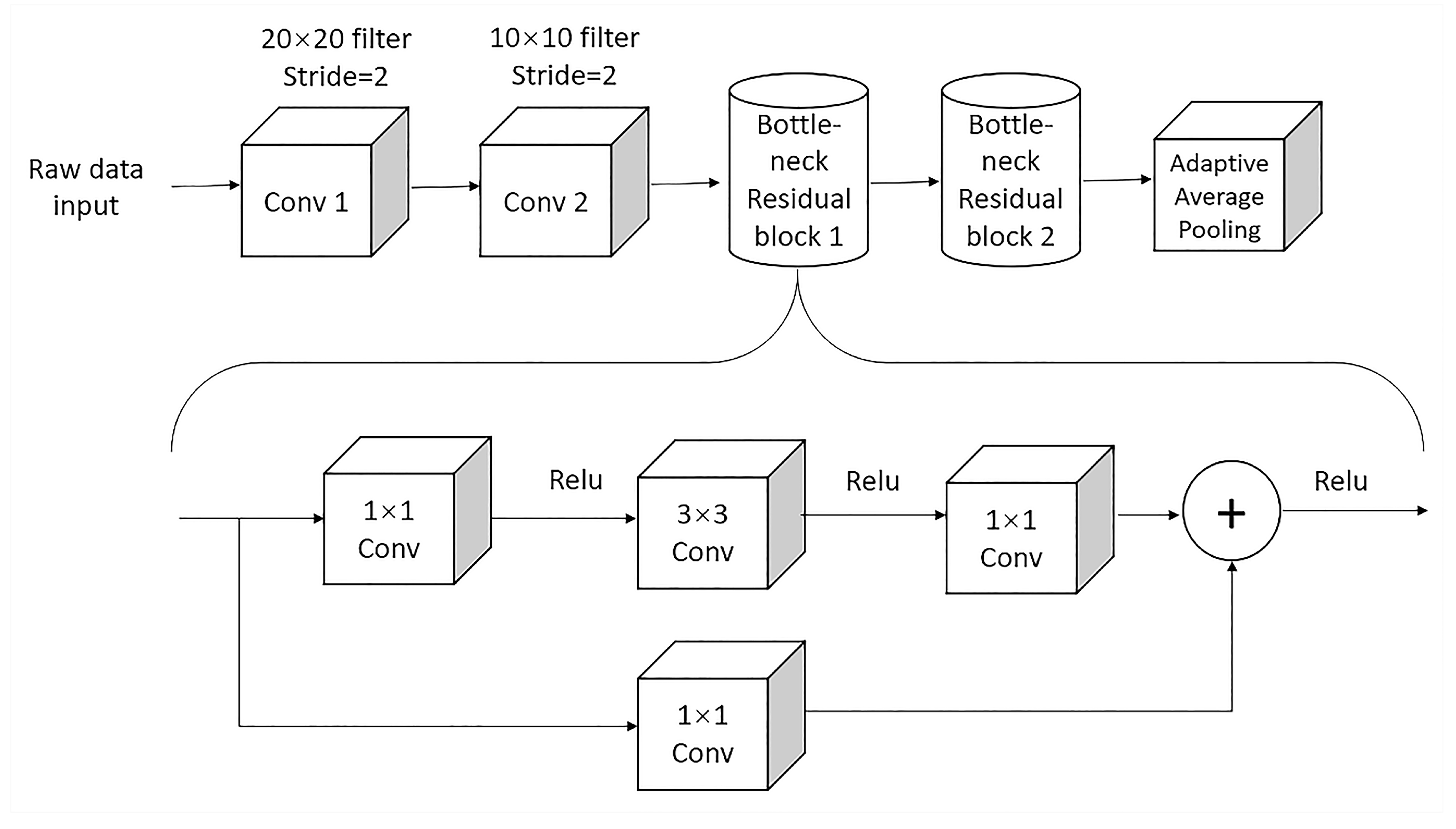
The feature extractor’s original structure includes two residual blocks, each consisting of two convolution layers with a 3 × 3 convolution kernel for each. As a result, this structure generates many parameters, significantly reducing the models’ computational efficiency and increasing the risk of overfitting. To overcome these two issues, this project improves the structure of the feature extractor. This new structure remains two convolution layers. The first convolution layer contains a 20 × 20 filter, a bath normalization layer, a max pooling layer, and a Relu activation layer. The second convolution layer consists of the same layers as the first convolution layer, except for a 10 × 10 filter. This project has modified the structure of two residual blocks. Both of them comprise a 1 × 1 filter, a 3 × 3 filter, a 1 × 1 filter, and an identity map with a 1 × 1 filter. Finally, the final result is passed to the adaptive average pooling layer after going through a Relu activation layer.

Figure 4 represents the detailed structure of the improved feature extractor based on a bottleneck residual block, which consists of two components: residual mapping and identity [40]. The residual mapping is the main component of the structure. It is utilized for learning the transferable and robust features of the input tensor and producing the residual function F(x). This function is added back to the input tensor to produce the output of the block. In this figure, one 1 × 1 convolutional layer, one 3 × 3 convolutional layer, and one 1 × 1 convolutional layer make up the component of residual mapping. Specifically, the first 1 × 1 convolutional layer reduces the quantity of input tensor channels. In comparison, the second 1 × 1 convolutional layer is utilized to restore the number of channels to the original value. By applying this residual mapping, the whole set of variations in the main convolutional layer will be reduced, resulting in a low computational cost of the block. The 3 × 3 convolutional layer plays a critical part in the residual mapping, where it operates on the reduced-channel input tensor and is utilized for learning the input data’s underlying features.

The identity part in the bottleneck residual block is the shortcut connection, which enables the addition of the block’s output to the input tensor. This connection can ensure that the network can learn identity mapping, which is very important for achieving good performance on a wide range of tasks. The identity part of the block involves adding the input tensor to the output of the residual mapping:

$$y=F(x,W_i)+x$$

(11)

where the input vector is represented as x, and the output vector is denoted as y in the bottleneck residual block. If x and F have the same dimensions, Equation (11) is utilized. Otherwise, to match the dimensions, a linear projection Ws using shortcut connections is carried out:

$$y=F(x,W_i)+W_{s}x$$

(12)

where $W_s$ denotes a square matrix for matching the dimensions between input x and output y. The residual mapping function is:

$$F(x,W_i)=W_3\sigma \left(W_2\sigma \left(W_{1}x\right)\right)$$

(13)

where F denotes residual mapping, $\sigma$ represents the activation function Relu, and the biases are eliminated to simplify the notations.

The pseudocode of this improved feature extractor is shown in Appendix A. In Algorithm A1, a feature extractor based on the bottleneck residual block is defined by the pseudocode. It is made up of two primary parts, a feature extractor module and a residual block. The ResNet building block, which is a well-liked building block in deep learning architectures, forms the foundation for the residual block in the code. It is intended to make it possible for a deep learning network to quickly and efficiently extract more robust and useful features from bearing fault data to improve classification accuracy. The block accepts an n × c × l tensor as input, where n stands for the batch, c for the number of input channels, and l for the sequence quantity. The first 1 × 1 convolutional layer applies the 1D convolution process. When the convolutional layer is complete, batch normalization normalizes the features and increases model convergence. After batch normalization and the Relu activation function, the second convolutional layer receives the first 1 × 1 convolutional layer’s output. The second one has a 3 × 3 filter and one padding. Following batch normalization, the third convolutional layer with a 1 × 1 kernel size is used to restore the reduced number of channels to their original size. Before applying the final activation function, the short connection adds the input tensor to the third convolutional layer’s output.

The feature extractor module defined in the code applies two sequential convolutional layers with batch normalization and Relu activation, followed by two residual blocks responsible for extracting and refining the features from the raw input data. The adaptive average pooling is utilized to reduce the feature map’s spatial dimensions to 1, and a flattened layer is applied to reshape the output tensor. Finally, a dropout layer with a probability of 0.5 is applied to the output tensor to prevent overfitting during training. The forward method of the feature extractor module takes an input tensor and applies the defined layers in a sequential manner for extracting features from the input data, producing an output tensor size.

4. Experiment Result Analysis

4.1. Experiment Settings

In order to test this improved feature extractor, two popular models, domain adversarial neural networks (DANN) and maximum classifier discrepancy (MCD), were selected for conducting binary classification on vibration signal data from two fault diagnosis data sets, CWRU and XJTU. The source data was collected in CWRU. Target data was collected from a complete run-to-failure data set, XJTU [43]. The labels of the target data were removed before feeding source and target data into DANN and MCD. In this experiment, 0 was utilized to represent the class of the inner race, and 1 was utilized to represent the class of the outer race. All the samples were the same for DANN and MCD models during training and testing. In addition, maximum classifier discrepancy (MCD) was applied to pseudo-label semi-supervised learning. Finally, several comparison experiments were conducted using the maximum classifier discrepancy model.

4.2. Data Selection

4.2.1. Source Domain Data Set

The source data was collected from the CWRU data set in this project due to three accelerometers, including fan-end bearing accelerometers, base-plate accelerometers, and drive-end bearing accelerometers, which can be used for collecting vibration signals of different bearings. Electrical discharge machining (EDM) can automatically create seeded faults in the bearing. The bearing fault types contained inner and outer races with three distinct inches (0.07 mm, 0.014 mm, and 0.021 mm) collected from 48 k drive end bearing fault data. The fault diameters of the inner race used in this experiment were 0.07 mm, 0.014 mm, and 0.021 mm, and their motor speed was 1730 rpm. The outer race’s fault diameters and motor speed were identical to the inner race. The position relative to the Load Zone of the outer race was centered at 6:00. Additionally, the motor load for both inner and outer races was 3 hp.

Table 1. The details of the source data.

Fault Type	Fault Diameter (mm)	Motor Load (HP)	Motor Speed (rpm)	Data Size	Sampling Frequency (Hz)	Outer Race Position	Class Label
Inner Race	0.007	3	1730	480,000	48 k	*	0
Inner Race	0.014	3	1730	480,000	48 k	*	0
Inner Race	0.021	3	1730	480,000	48 k	*	0
Outer Race	0.007	3	1730	480,000	48 k	Centered at 6:00	1
Outer Race	0.014	3	1730	480,000	48 k	Centered at 6:00	1
Outer Race	0.021	3	1730	480,000	48 k	Centered at 6:00	1

* denotes null.

shows the detail of the data:

4.2.2. Target Domain Data Set

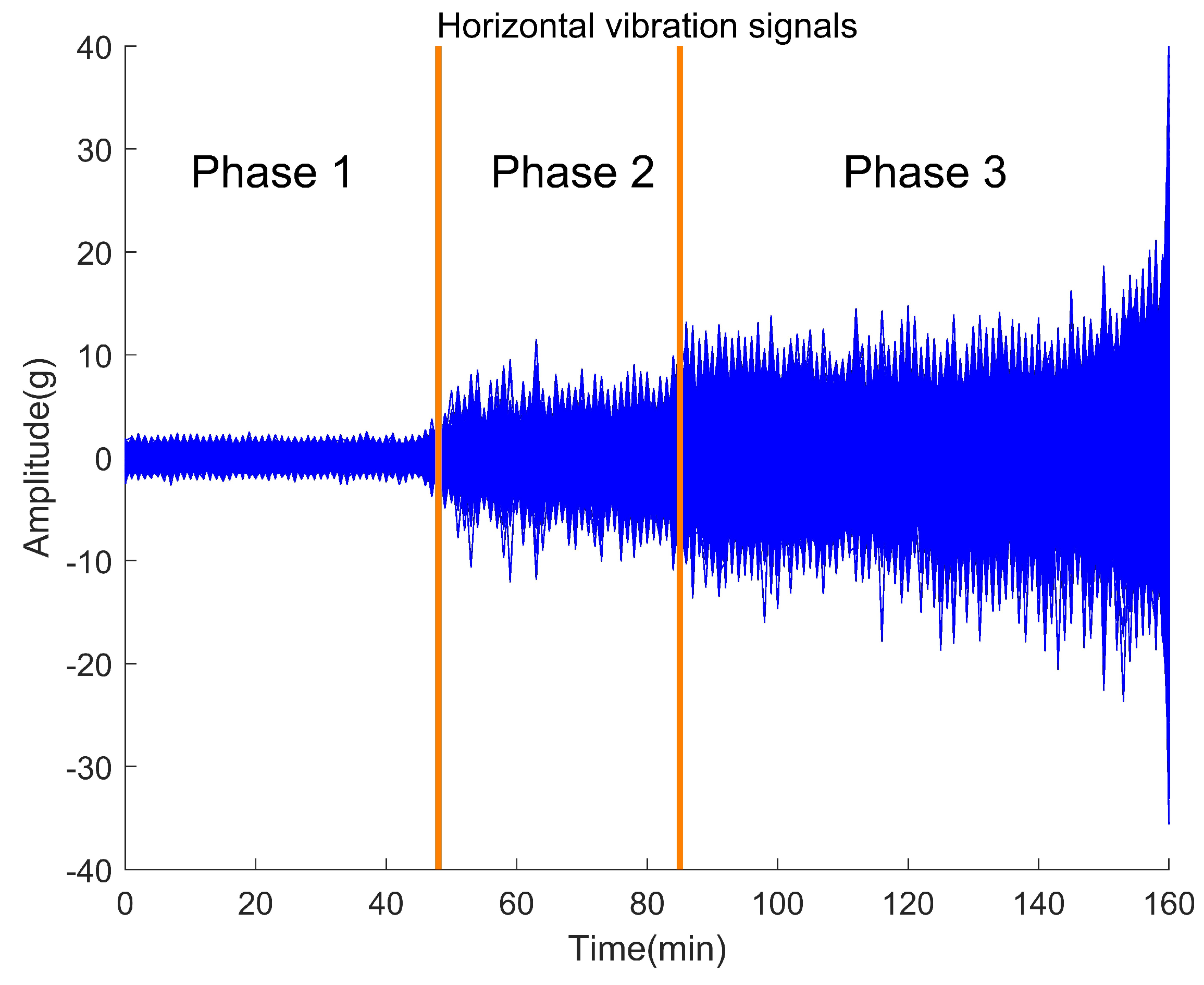
The target data was complete run-to-failure data obtained through accelerated degradation experiments selected from the XJTU data set [43]. The bearing degradation reflected in the data well simulates the bearing degradation in the real world. Figure 5 shows the data used from the target data set. Figure 6 shows the target data observed in the full process of bearing deterioration, from their normal state to frequent failures. In this project, the fault state was used experimentally.

Table 2. The details of the target data.

Fault Type	Data Set Name	Fault Diameter (mm)	Operating Condition	Normal State Range (min)	Fault State Range (min)	Data Size	Sampling Frequency (Hz)	Class Label
Inner Race	Bearing 2_1	29.30	2250 rpm (37.5 Hz) and 11 kN	1–452	454–484	982,000	25.6 k	0
Inner Race	Bearing 3_3	29.30	2400 rpm (40 Hz) and 10 kN	1–340	341–369	982,000	25.6 k	0
Inner Race	Bearing 3_4	29.30	2400 rpm (40 Hz) and 10 kN	1–1416	1417–1514	982,000	25.6 k	0
Outer Race	Bearing 2_2	39.80	2250 rpm (37.5 Hz) and 11 kN	1–50	51–159	982,000	25.6 k	1
Outer Race	Bearing 2_4	39.80	2250 rpm (37.5 Hz) and 11 kN	1–30	31–40	982,000	25.6 k	1
Outer Race	Bearing 2_5	39.80	2250 rpm (37.5 Hz) and 11 kN	1–120	121–337	982,000	25.6 k	1
Outer Race	Bearing 3_1	39.80	2400 rpm (40 Hz) and 10 kN	1–2463	2464–2536	982,000	25.6 k	1
Outer Race	Bearing 3_5	39.80	2400 rpm (40 Hz) and 10 kN	1–10	11–110	982,000	25.6 k	1

provides information on target data, such as fault type, data set, fault diameter, operating condition, normal state range, fault state range, data size, sampling frequency, and class label. The important thing to note is that the class labels of target data are removed when training.

4.3. Preprocessing Data

In the experiment, preprocessing is critical for preparing the input data for DANN and MCD. The preprocessing stage involves retrieving source and target instances, loading and separating data and labels, applying the downsampling technique, reshaping the data to match the models’ input shape, and storing the preprocessed data. This prepares the data for training the models and aims to improve their performance. The details are shown below.

Figure 7 represents the detailed process of data preprocessing. The first stage is to retrieve source and target instances from the CWRU and XJTU data sets. After that, loading the data is a step responsible for reading and separating data and labels from instances obtained from these two data sets. Then the downsampling technique is applied to the source and target data to reduce the dimensionality of the data. Data after reduced dimension and label arrays are utilized as inputs to reshape the length of 1-dimensional signal data to 1000 to match the expected input shape of the two models. Finally, the reshaped data and labels are stored in arrays for feeding into two models. In the model training, source and target data with labels will be fed into two models to update the weights to achieve convergence.

A specific window length of 1000 is considered for 1-dimensional signal data. A window is a subset of consecutive data from the signal used for analysis. The input data is divided into overlapping or non-overlapping segments by selecting a window length to allow the network to capture local patterns and relationships within the signal. However, it does not address the processing of several sensor signals from different sensors. Multiple sensor signals can be handled as multiple channels in the input data. This means multiple dimensions represent each sensor signal instead of having a single dimension for the input signal data. Each dimension corresponds to a specific channel to allow the network to process and learn from different sensor data simultaneously.

When dealing with 1-dimensional signal data, a technique involves applying 2-dimensional kernels along the time axis of the signal. This is achieved by treating the kernel as a sliding window that moves along the signal. A convolution operation occurs at each step, where the values within the window are combined with the corresponding kernel values. This process captures meaningful features and patterns in the signal, yielding a new output value at each step. Using 2-dimensional kernels enables the examination of local trends, edges, and other interconnected structures that may span neighboring time points within the 1-dimensional signal data.

4.4. Outcomes of Domain Adversarial Neural Network

For training DANN, all input data is marked as domain labels. The target data are designated 1, whereas the source domain data are marked as 0. The line chart below shows DANN’s accuracy, domain loss, and classifier loss with the improved feature extractor during 200 training epochs.

Figure 8 gives information about the accuracy and loss of the DANN with a bottleneck residual block. It is clear that the best accuracy in this model is 96.84%, but the accuracy curve oscillates significantly. In comparison, the domain loss and classifier loss curves become stable at 0.75 and 0.3, respectively, after some training epochs. Various potential reasons warrant discussion, among which data set differences emerge as a notable factor. Notably, the quantity of two data sets used in the experiment represents acceleration. It is worth considering that the CWRU and XJTU data sets may exhibit distinct characteristics, such as fault types, levels of noise, and signal-to-noise ratios. The CWRU and XJTU data sets may have different characteristics, such as fault types, levels of noise, and signal-to-noise ratios. These differences can cause the DANN to struggle with domain adaptation due to the possibility that it would be unable to accurately capture the variations between these two domains. Consequently, the accuracy curve oscillates when this model tries to adapt to the target domain. Another reason may be domain shift. A domain shift may occur if the distributions between these two domains cannot match. This can also cause the DANN to struggle with domain adaptation, as the effective generalization of this model is impossible.

However, relying solely on the maximum accuracy could be misleading if the accuracy values exhibit significant fluctuations. It is possible that the maximum accuracy is a result of chance or randomness during the training process rather than a consistent and reliable representation of the model’s true performance. So, the average accuracy of the DANN model is also calculated to provide a more valid assessment of the DANN’s overall performance. The average accuracy in this model is 63.77%.

The measurement of the domain loss is the distance of these two distinct domains. In comparison, the explanation for classifier loss is an index, which measures the accuracy difference of different classifiers on the objective data. In the training process, these two measures need to be optimized simultaneously. If the domain loss becomes stable, it indicates that the DANN model has effectively adapted the target domain from the source domain. When this index of classifier loss tends to be stable, it indicates that the model has learned to classify the data accurately.

4.5. Outcomes of Maximum Classifier Discrepancy

The MCD model also is selected for testing this improved feature extractor. For training the MCD, 0 indicates the category of source data, and 1 indicates the category of target data. Furthermore, this paper has applied pseudo-label semi-supervised learning in MCD. The following line chart represents the testing accuracies and discrepancy loss of MCD and MCD with the pseudo label in 100 epochs. The details are shown below.

Figure 9 gives information about the accuracies of MCD and MCD with the pseudo label. In the first chart, the changes in the accuracy of classifier 1 are almost the same as in classifier 2. After 30 epochs of training, the classification accuracy of MCD achieves over 90% and remains stable. In the second chart, the accuracies of classifiers in MCD with the pseudo label fluctuate around 90%. However, the accuracies of these two classifiers are different. It is easy to determine that classifier 1 achieves higher accuracy than classifier 2. This difference may be because they are trained in a mixed domain. At the same time, they are optimized for minimizing the domain losses for both domains. Furthermore, the pseudo-labeling process in MCD with the pseudo-label introduces additional noise and uncertainty into the training data, which can lead to different classifiers and different accuracies.

Figure 9 represents the discrepancy loss from MCD and MCD with the pseudo label. It is clearly shown that the discrepancy loss of MCD remains below 0.05. As training continues, its discrepancy loss approaches 0. In contrast, the discrepancy loss of MCD with the pseudo label fluctuates wildly between 0 and 0.3. As training continues, its discrepancy loss fluctuates slightly but is still unstable. The fact that the feature distributions in these two distinct domains are aligned using discrepancy loss, which is determined using the variances between the model’s predictions on these data, might be one explanation for this. However, in MCD with the pseudo label, pseudo-labels are used to designate data not labeled in the objective domain, which introduces some noise into the training data. As a result, the discrepancy loss in MCD with the pseudo label can fluctuate more wildly than that of MCD as the model tries to adapt to the noisy and uncertain pseudo labels and align the feature distributions in these two domains. Consequently, the optimization process may become more challenging and unstable as the model seeks to reconcile the conflicting goals of matching the feature distributions with minimized losses in these two domains.

The table below gives more details for comparing MCD with MCD using pseudo-label semi-supervised learning. This strategy allows test samples with pseudo labels to be added to the data set when training this model. The details are shown below.

Table 3. The details of training strategies used in MCD.

Training Strategies	Average Accuracy	Best Accuracy	Average Discrepancy Loss	Training Time
Without pseudo label	79.36%	100%	0.012	139s
With pseudo label	94.19%	100%	0.093	139s

gives information about the average accuracy, best accuracy, average discrepancy loss, and training time of MCD using different training strategies. The best testing accuracy for both strategies is 100%. The average accuracy of the model using pseudo labels is 94.14%, which is approximately 15% higher than the model without pseudo labels. MCD can improve average accuracy with pseudo-labeling because pseudo-learning allows the model to use unlabeled data, which can provide additional detail about the distribution of the underlying data that can be used to make more accurate predictions. In addition, pseudo-tags can help regularize models, reduce overfitting, and improve accuracy. In addition, the average discrepancy losses for these two strategies are 0.015 and 0.093, respectively, and the training time for both is 139 s.

4.6. Transferability Estimation

This paper compares the transferability of different models, such as the baseline model based on random forest, logistic regression with cross-validation, deep autoencoder sparse network (DASN), support vector machine (SVM), DANN, and MCD. The details are shown below.

Table 4. Transferability estimation of different models.

Training Strategies	Best Accuracy
Baseline	52.13%
DASN	69.30%
DANN with the standard residual block	94.40%
MCD with the standard residual block	98.17%
DANN with the bottleneck residual block	96.84%
MCD with the bottleneck residual block	100%

shows the testing accuracy of different models based on CWRU and XJTU data sets [40]. The baseline model achieves the lowest accuracy in this table, only 52.13%. DASN achieves 69.30%. The accuracies for DANN and MCD with an old feature extractor are about 94.40% and 98.17%, respectively. The accuracies for DANN and MCD with an improved feature extractor in this project achieve 96.84% and 100%, respectively.

To train the baseline model, only the source data is needed, and the model is then applied to the target data to conduct binary classification. This baseline model is based on logistic regression CV. Logistic regression CV is a method for training a logistic regression model, a classification algorithm. It is similar to regular logistic regression but with an additional step of performing cross-validation to tune the regularization parameter. This allows the model to find a balance between model complexity and overfitting, resulting in improved performance compared to regular logistic regression. The trained model can then be used to make predictions on new data.

The MCD model achieves the best accuracy compared with other methods. The DANN model ranks second place, but the accuracy curve of this model is violently oscillating. When the MCD model utilizes pseudo-label semi-supervised learning, it achieves a better average correct rate, and the correct rate curve is smoother. To evaluate the transferability of different models, this project utilized fault diagnosis data sets to train several popular models and compare their classification accuracy. The lowest requirement for the results of the DANN and MCD models is that they are higher than those of the baseline model. Otherwise, these models will have negative transferability and will be unfeasible. Finally, these revised models should achieve high enough average accuracy on the test data set.

5. Conclusions and Future Work

In this paper, an improved feature extractor structure has been put forward, and two popular networks, DANN and MCD, were selected for testing this revised feature extractor. The result has shown that with the help of the improved feature extractor, both DANN and MCD can well classify vibration signal data in fault diagnosis data sets, CWRU and XJTU, and these two models have achieved classification accuracies of 96.84% and 100%. Pseudo-label semi-supervised learning was also utilized in MCD, resulting in improved performance on average accuracy, achieving 94.19%. Finally, this research selected several popular models and estimated their transferability. The result has shown that the MCD with the improved feature extractor achieved the highest classification accuracy. DANN ranked in second place, but its accuracy curve oscillated significantly. Finally, pseudo-label semi-supervised learning was useful and achieved higher average accuracy on the test data set.

This paper identifies several areas that could be investigated to improve these two networks, DANN and MCD, with the improved feature extractor. First, future research could focus on the multi-mode fault diagnosis data. This paper considers the vibration signal data and conducts binary classification on vibration fault data sets. If multi-mode faults are under consideration, fault diagnosis networks can quickly and accurately identify the fault type and provide a solution. This can avoid property damage to the greatest extent and maintain the lasting stable operation of the machinery. Secondly, imbalanced data should be under consideration in the future. In this paper, source data is gathered from CWRU, and target data is gathered from the XJTU. Both of these are balanced data sets. However, imbalanced data is more common in actual production and life. When dealing with these data, the current network could achieve low performance and classification accuracy. So, how to improve these two networks for adapting imbalanced data is another future direction. Additionally, information loss should be considered in future research. In this paper, a bottleneck residual is utilized in the improved feature extractor. During the process of reducing the channels of input vectors, it could cause information loss.

In addition, it has been observed that the proposed improvements to the feature extractor bring only marginal performance gains to already well-performing methods and applications. However, the applicability of this modified feature extractor to data sets with low predictability requires further examination. To evaluate its performance on such data sets, several strategies can be employed, including cross-domain validation, and transfer learning and domain adaptation. Cross-domain validation involves assessing the feature extractor’s performance on diverse data sets from various domains and measuring its generalization capabilities. This approach enables researchers to predict its performance across different domains and determine if the modification consistently improves classification accuracy. On the other hand, transfer learning and domain adaptation involve fine-tuning the feature extractor using pre-trained models on established data sets to analyze its adaptation capabilities and performance in domains with different statistical properties. These strategies provide avenues for evaluating the modified feature extractor’s performance and predicting its suitability for data sets with lower predictability.

Finally, future research may look forward to the development of an explainable framework [44]. This framework could integrate additional sensor types, such as acoustic and temperature, to enhance the model’s accuracy. Additionally, it could be applied to predict the future behavior of the fault system to enable proactive maintenance and prevent catastrophic failure. Addressing these future research directions can improve the fault diagnosis model’s accuracy and applicability, making it suitable for deployment in real-world industrial systems.