A Histopathological Image Classification Method Based on Model Fusion in the Weight Space

Abstract

Automatic classification of histopathological images plays an important role in computer-aided diagnosis systems. The automatic classification model of histopathological images based on deep neural networks has received widespread attention. However, the performance of deep models is affected by many factors, such as training hyperparameters, model structure, dataset quality, and training cost. In order to reduce the impact of the above factors on model training and reduce the training and inference costs of the model, we propose a novel method based on model fusion in the weight space, which is inspired by stochastic weight averaging and model soup. We use the cyclical learning rate (CLR) strategy to fine-tune the ingredient models and propose a ranking strategy based on accuracy and diversity for candidate model selection. Compared to the single model, the weight fusion of ingredient models can obtain a model whose performance is closer to the expected value of the error basin, which may improve the generalization ability of the model. Compared to the ensemble model with n base models, the testing cost of the proposed model is theoretically $1/n$ of that of the ensemble model. Experimental results on two histopathological image datasets show the effectiveness of the proposed model in comparison to baseline ones, including ResNet, VGG, DenseNet, and their ensemble versions.

1. Introduction

Histopathological images are digital images of tissue sections observed under a microscope, and a large number of studies have shown and verified their important value in biomedicine [1,2]. In particular, histopathological images have been broadly used in the screening of many cancers and are, in fact, considered the gold standard for diagnosing a significant number of cancers. One notable feature of histopathological images is their high information density, which may include microstructures, such as cells, nuclei, stroma, tumors, blood vessels, glands, etc., and histopathological images can be observed at various magnifications, allowing for a multi-scale analysis [3].

The automatic classification of histopathological images plays an important role in computer-aided diagnosis (CAD) systems, which can reduce the burden of pathologists, decrease the influence of human factors in diagnosis, and improve the stability of the results. With the rapid development of deep learning theory and technology [4,5,6,7], histopathological image classification models based on convolutional neural networks have exhibited excellent performance in many applications. In order to improve the inference performance of convolutional neural networks, models with a larger number of layers and channels have been designed. For example, in the famous ImageNet image classification challenge [8], the number of parameters of CoAtNet-4+PT-RA-E150 [9], one of the state-of-the-art models at present, reaches 275M. Large-scale models have high requirements when it comes to the size of the training dataset and the capabilities of computer hardware. However, obtaining a large number of histopathological images is not an easy task for certain medical departments. It is also difficult to fully satisfy the computing resources required to train the model.

Different strategies have been proposed to solve the contradiction between the lack of training data and computing resources and the pursuit of model performance. One widely used strategy is transfer learning. It takes the approach of further training (fine-tuning) on top of a well-trained model, e.g., models trained on ImageNet. A common practice is to train only the weights of the last few fully connected layers while fixing the weights of the remaining layers. By using a pre-trained model, one can make full use of its architecture and weights, resulting in significant reductions in the design and training costs of the model. This strategy has been widely used in work on histopathological image analysis [10,11,12,13,14,15]. However, setting the model hyperparameters becomes a challenge when using this strategy to train or fine-tune the pre-trained model. Common hyperparameters include the learning rate, weight decay rate, batch size, data augmentation strength, etc. Hyperparameters have a direct impact on the training effect of the model. The optimal hyperparameter setting is usually difficult to obtain. Instead, people determine hyperparameter settings based on experience or by using a grid search on a small verification set. However, the grid search requires a lot of computational resources and may not reach global optima. Another strategy is model ensemble. The main idea of model ensemble is to train several base models with diversity, and then perform majority voting or weighted voting on the output of these models to obtain the final results. By using different training sets, changing the training hyperparameters, using different types of optimizers, etc., the diversity between base models can be improved. Model ensemble can combine multiple base models with suboptimal performance into a model with strong overall performance, which can lead to better results than a single model, provided that the diversity among the base models is ensured. Although the model ensemble strategy avoids the computationally expensive hyperparameter search, it greatly increases the inference cost of the model. This is because each test sample needs to be fed to each base model for inference and, hence, the running time is proportional to the number of base models. This limits the application scope of the model ensemble methods, especially in low-specification terminals or mobile devices.

Recently, some studies on model fusion in the weight space have been proposed [16,17,18,19]. Researchers proposed different strategies to fuse weights of some trained/pre-trained models to form a single model. Equation (1) shows the weight average strategy for model fusion:

$$f_{fusion}(x,\theta )=f(x,\frac{1}{M}\sum _{k=1}^M{\theta }_k)$$

(1)

where $F=\{f(x,{\theta }_1),f(x,{\theta }_2),\cdots ,f(x,{\theta }_M)\}$ represents a set of trained models with the same architecture but different weights.

In contrast, model ensemble works in the model space, meaning that it fuses the output of the models to obtain a final result. Equation (2) shows the majority voting strategy on the model set F:

$$f_{ens}\left(x\right)=\frac{1}{M}\sum _{k=1}^{M}f(x,{\theta }_k)$$

(2)

It can be seen that the inference cost of $f_{fusion}$ is only $\frac{1}{M}$ of that of $f_{ens}$ while the training costs of both are almost equivalent. The rationale for model fusion in the weight space lies in the relationship between local minima and the global solution. Draxler et al. [20] claimed that the loss minima of a deep neural network are not isolated in a parameter space but rather form a connected manifold. There can be a path between two local minima where the loss does not significantly fluctuate. Izmailov et al. [16] observed that when training a deep neural network using a high-frequency cyclical learning rate (CLR) [21], the model weights corresponding to the periodic minimum learning rate are located on the periphery of the most desirable solutions (global loss minima). Averaging these weights may lead to a solution closer to the optimal solution than the ones located on the periphery. Wortsman et al. [17] extended the weight-averaging method from a single training trajectory to the context of fine-tuning models with different training hyperparameters. Their method can also work in the transfer learning mode.

Inspired by these studies, we propose a novel model-based fusion method for histopathological image classification tasks. Following the work of Wortsman et al. [17], we use the term soup in this paper to refer to the models fused in the weight space, and each model’s weights are referred to as the ingredients of the soup. We propose two strategies for constructing soup models: the average strategy and the dominant difference weight-averaging (DDWA) strategy. For DDWA, by drawing on the idea of the selective ensemble [22], we select ingredient models that perform satisfactorily enough on the validation set and have large differences from other models for fusion in the weight space. Compared to the strategy of averaging the weights of all ingredient models, DDWA can produce a fusion model that achieves a loss closer to the optimal expected loss. The proposed method can work either in the fine-tuned model mode or in the full model mode.

The contributions of this paper are two-fold:

• We introduce a weight-based model fusion strategy to solve the problem of histopathological image classification. The strategy significantly reduces the computational complexity of model training and inference.
• We propose the DDWA method to screen the ingredient models, enabling the weight fusion model to achieve a better approximation to the optimal value of the loss function’s error basin, thereby improving the generalization ability of the model.

The remainder of this paper is organized as follows. We review some related and important works in Section 2. In Section 3, we present the proposed model and its strategies. The evaluation results are reported and discussed in Section 4. Section 5 discusses the advantages and limitations of the proposed model. The paper is concluded in Section 6.

2. Related Works

The distribution of minima regions in the loss function of deep neural networks has been a subject of study in recent years. Draxler et al. [20] observed that along the paths connecting minima in the weight space, which are unrelated to each other, the training and test loss would remain nearly equal to that of the minima, while the test error slightly increases. Their work revealed that the distribution of local minima in the loss function of deep neural networks has certain characteristics. Smith and Topin [23] explored the topology of the loss function of ResNet-56 on the CIFAR-10 dataset by training with CLR and different fixed learning rates. Their work provides theoretical support for finding the optimal region of the loss function. Garipov et al. [24] further proposed an ensemble framework that consisted of models along high-accuracy paths in the weight space. They proposed a fast geometric ensemble (FGE) strategy, which first trains a model to about 80%, uses CLR or fixed learning rates for further training, records the model weights for every m iteration, and ensembles these recorded models for final results. Izmailov et al. [16] proposed stochastic weight averaging (SWA) by simply averaging the model weights at each recorded point along the trajectory of a stochastic gradient descent (SGD) procedure, with CLR or fixed learning rates. Their work is based on the observation that SGD methods generally converge on the edge of the minima basin. In such cases, weight averaging can lead to a better solution. Jain et al. [25] presented a theoretical analysis of tail-averaging in machine learning models. They presented the generalization error bounds of different weight-averaging strategies in the SGD procedure. Recently, Guo et al. [26] revisited SWA and pointed out that its effectiveness depends on the extent to which the SGD algorithm runs before converging. Their work indicated that fusing models in the weight space can reduce the test variance.

Neyshabur et al. [27] proposed that when a pre-trained model is fine-tuned on a new training dataset using different hyperparameters, the model instances would stay in the same loss landscape basin. Moreover, these fine-tuned instances would be similar in feature spaces and close in parameter spaces. Based on their work, Wortsman et al. [17] proposed model soup, which performs weight fusion over a series of fine-tuned models trained with different hyperparameters. They designed three strategies for weight fusion: average soup, greedy soup, and learned soup. These strategies utilize averaging, selective fusion, and weighted combination to obtain the soup model. For the greedy soup strategy, one would test each ingredient and keep it if its addition improves the performance of the soup model. For the learned soup strategy, one would search for a weighted combination that makes the model perform optimally on the test set. Inspired by their work, in this paper, we introduce the soup model into the histopathological image analysis and propose a novel weight fusion strategy by drawing on the idea of selective ensemble.

As an effective strategy for improving the model performance and reducing variance, ensemble learning has been widely used in histopathological image analysis. Hameed et al. [28] fine-tuned 4 pre-trained models based on VGG16 and VGG19. They then constructed an ensemble model by averaging the prediction probabilities of the 4 models. The ensemble model outperformed the individual models in terms of test loss. Sohail et al. [29] proposed a method based on deep ensemble for the analysis of mitoses in breast histopathology images. First, they selected candidate mitoses via an instance segmentation method based on deep learning. Then a heterogeneous ensemble of deep CNNs was run for mitotic nuclei classification. Kumar et al. [30] proposed the stacked generalized ensemble model for breast cancer classification, which uses 6 deep networks as level-0 models and logistic regression as a level-1 model. The level-1 model acts as an integrator for the outputs of sub-models. Their model achieved competitive results in the invasive ductal carcinoma dataset. Ref. [31] proposed a model that uses a deep transfer learning network to detect COVID-19 from lung CT scan slices, which can make full use of the supervised information in the dataset of the source field, and is more effective for application scenarios where there are inadequate amounts of labeled data in the target fields. Ref. [32] used deep neural networks with different architectures, implemented with contrast-limited adaptive histogram equalization, to detect COVID-19 from CT lung scans. Their work demonstrates the effectiveness of deep neural networks in detecting COVID-19. In [33], the authors designed a weighted average-based heterogeneous network for detecting COVID-19 from chest CT scans and chest X-ray images. They fine-tuned different deep neural networks, such as VGG19, ResNet101, and DenseNet169, as base classifiers, and then integrated the best-performing models to obtain the final results. This work demonstrates that ensemble learning based on model fine-tuning is effective for COVID-19 detection.

In [28,29,30], it can be seen that the ensemble of different deep neural networks has been extensively utilized in histopathological image analysis. The limitations of these works are listed as follows: (1) They greatly increase the inference costs of the models because they must obtain the results from each model for ensemble learning; (2) different deep neural networks need to be carefully designed to maintain the diversity in ensemble learning, which greatly influences the last outcome. Therefore, the DDWA model is proposed to overcome these limitations. In addition, studies on histopathological image analysis based on model weight fusion are rarely publicly reported. Our study can be used as a complement to the existing work in the field of weight fusion methods for histopathological image analysis to a certain extent.

3. Model Fusion in the Weight Space for Histopathological Image Classification

3.1. Basic Model Training

As indicated by previous studies [16,20,25,27], model fusion in the weight space works well in models from snapshots of the trajectory of an SGD procedure, or from fine-tuned pre-trained models with different hyperparameters. We applied both methods to generate basic models (ingredient models for soup) in this study. Specifically, we used three famous deep convolutional neural network architectures, i.e., ResNet [34], VGG [35], and DenseNet [36], for basic model training. All models were pre-trained on the ImageNet-1000 dataset [8] and, hence, our model works in the fine-tuning mode.

The pre-trained models were fine-tuned with two training settings, i.e., the cyclical learning rate and different training hyperparameters. We saved the model weights in both cases as the potential ingredients for model fusion.

A. Ingredient Model Training with Cyclical Learning Rate

The main idea of the cyclical learning rate (CLR) [21,23,24], which is different from the traditional learning rate-adjusting strategy, which decreases monotonically, is to vary the learning rate cyclically within a proper range as the number of training epochs increases. Let ${\alpha }_1$ and ${\alpha }_2$ represent the lower and upper bounds of the learning rate; the CLR strategy changes the learning rate according to the iteration number k, as shown in Equations (3) and (4):

$$\alpha \left(k\right)=(1-t_k){\alpha }_1+t_k{\alpha }_2$$

(3)

$$t_k=\frac{mod(k-1,c)+1}{c}$$

(4)

In Equation (4), c represents the length of a cycle. Here, we refer to processing a mini-batch of data at a time as an epoch. At the end of each cycle, i.e., when the learning rate reaches the minimum, the model weights are saved as checkpoints. Note that ${\alpha }_1$, ${\alpha }_2$, and c are hyperparameters for model training, and have a great impact on the effectiveness of model weight averaging. The maximum learning rate ${\alpha }_2$ must be able to jump out of a local minima basin, which determines the exploration ability of the model. In this study, we set ${\alpha }_2$ to a slightly larger value than the initial learning rate used in the traditional learning rate decay training strategy. The minimum learning rate ${\alpha }_1$ and the length of a cycle c are set according to [24].

B. Ingredient Model Training with Different Training Hyperparameters

In addition to CLR, we also fine-tuned the pre-trained model with different (but constant) learning rates with data augmentation. For constant learning rates, we set the learning rate to $0.0001$, $0.0015$, and $0.0002$, respectively. We used RandAugment [37] for data augmentation, which aims to reduce the parameter space and maintain the diversity of data (images) by using a non-parametric process instead of the learning strategy and probability. There are only two parameters involved when using RandAugment, i.e., the number of transformations N and the degree of augmentation distortion M. RandAugment makes use of a linear scale to represent the intensity of each conversion. Simply put, each transformation is in the integer range of 0 to 10, where 10 represents the maximum range of a given transformation. The larger the values of N and M, the stronger the degree of regularization. We set $N=9$ and $M=2$ in all of the experiments in this study.

C. The Effectiveness of Soup Ingredients

The effectiveness of model fusion in the weight space depends on whether the model weights are located in the same loss basin. To show that the ingredients obtained through our two training strategies meet the requirement of fusion in the weight space, we will first provide a formal definition of the loss basin, and then use a linear interpolation method for validation. We use the definition of loss basin proposed in [27], which can be formally written as follows:

Definition 1. 

Let $L:R^n\to R^{+}$ be a loss function and $S\subseteq R^n$ be a closed convex set, then S is a $(\epsilon ,\delta )–$basin for L if and only if the following holds:

• Let $U_S$ represent the uniform distribution over S, and $v_{S,L}$ represent the expected value of L on samples drawn from $U_S$. Then

  $${\mathbb{E}}_{w\sim U_S}\left[\right|L\left(w\right)-v_{S,L}\left|\right]\le \epsilon$$

  (5)
• $\forall w_1,w_2\in S$, define $h(w_1,w_2)=w_1+\tilde{\alpha }(w_2-w_1)$, where $\tilde{\alpha }=max\alpha |w_1+\alpha (w_2-w_1)\in S$. Then

  $${\mathbb{E}}_{w_1,w_2\sim U_S,p\sim \mathcal{N}(0,({\delta }^2/n)I_n)}[L(f(w_1,w_2)+p)-v_{S,L}]\ge 2\epsilon$$

  (6)
• Let $\kappa (w_1,w_2,p)=f(w_1,w_2)+\frac{p}{\left|\right|f(w_1,w_2)-w_1{\left|\right|}_2}(f(w_1,w_2)-w_1)$. Then

  $${\mathbb{E}}_{w_1,w_2\sim U_S,p\sim \mathcal{N}(0,{\delta }^2)}\left[L\right(\kappa (w_1,w_2,\left|p\right|\left)\right)-v_{S,L}]\ge 2\epsilon$$

  (7)

The definition of basin implies that, on the one hand, a basin should be relatively flat (small variance), and the value of the loss function that corresponds to each point in it should be close to the expected value. On the other hand, the value of the loss function corresponding to the points around the basin should be higher than the expected loss. Specifically, Equation (6) stipulates that the values of the loss function associated with the points within the basin should be higher than the expected values when Gaussian noise is added. Equation (7) stipulates that if a point within the basin is manually pushed away from the basin by a short distance, the value of its loss function should increase.

To validate the effectiveness of the ingredients, we use linear interpolation between two ingredient models parameterized by $w_1$ and $w_2$ to generate k middle points $w_i(1\le i\le k)$, where $w_i$ is given by

$$w_i={\gamma }_i{w}_1+(1-{\gamma }_i)w_{2}0\le {\gamma }_i\le 1$$

(8)

If $L\left(w_i\right)-\frac{L\left(w_1\right)+L\left(w_2\right)}{2}<\tau$ holds for all $w_i(1\le i\le k)$, in which $\tau$ is a threshold, it can be inferred that $w_1$ and $w_2$ are in the same basin. We report the results of the proposed model in Section 4.

3.2. Soup Strategies

Recent studies have shown that the way in which the model weights are generated and the method used for weight fusion have significant impacts on the performance of the soup model. We collectively refer to the generating and fusing of soup ingredients as soup strategies. We implemented two strategies for building the soup model. The first strategy was averaging the soup, which simply involves averaging the weight of each gradient in the soup. The weight-averaging strategy was applied and proved effective in previous studies. Since models trained using methods such as gradient descent often converge near the edge of the error basin, the use of the averaging strategy holds promise in moving a model closer to the center (expected value) of the error basin, which may have better generalization ability. Fine-tuning a pre-trained model with different training hyperparameters and recording the weights in each case would result in a set of models located in the same low-loss basin. The second strategy involves the use of dominant difference weight averaging (DDWA), which is motivated by the classical ensemble pruning method [38]. According to the classification accuracy $acc$ and diversity $div$, DDWA selects the ingredients with better performance to construct the soup model. Let $H=\{h_{w_1},h_{w_2},\cdots ,h_{w_M}\}$ represent the set of candidate ingredients and $D=\{(x_1,y_1),(x_2,y_2),\cdots ,(x_n,y_N)\}$ represent the evaluation dataset, where $x_i$ represents the ith instance and $y_i$ represents the corresponding class label. The ith ingredient’s $acc$ and $div$ are defined as Equations (9) and (10):

$$ac{c}_i=\frac{1}{N}\sum _{j=1}^{N}L(h_{w_i}\left(x_j\right),y_j)$$

(9)

$$di{v}_i=\frac{{\displaystyle \sum _{j=1}^N}{(h_{w_i}\left(x_j\right)-av{g}_j)}^2·\alpha }{N}$$

(10)

$$av{g}_j=\frac{1}{M}\sum _{k=1}^M{h}_{w_k}\left(x_j\right)$$

(11)

where $L(·,·)$ is a zero-one loss function, $av{g}_j$ is the averaging output of all candidate ingredients on $x_j$, and $\alpha =1$ if $h_{w_i}\left(x_j\right)$ equals the ground truth label $y_j$; otherwise, $\alpha =0$. $di{v}_i$ evaluates the difference between the ith component and the entire set under the condition of correct classification. We sort all of the ingredients using non-dominated sort (NDS) according to these two indices, and select the top q% of ingredients to build the soup model, as shown in Algorithm 1.

Algorithm 1: Non-dominated sort.

Input:  $ran{k}_A$: $acc$ ranking of M candidate ingredients  $ran{k}_D$: $div$ ranking of M candidate ingredients  H: candidate ingredients Output: $ran{k}_{NDS}$: $NDS$ ranking of M candidate ingredients  1: $F=\varnothing ,ran{k}_{NDS}=\varnothing$  2: for $i=1,2,\cdots ,M$ do  3:    $S_i=\varnothing$, $b_i=0$  4:    for $j=i,2,\cdots ,M$ do  5:      if $h_i$ dominates $h_j$ then  6:         add $h_j$ to $S_i$  7:      else if $h_j$ dominates $h_i$ then  8:         $b_i=b_i+1$  9:      end if 10:    end for 11:    if $b_i=0$ then 12:      Add $h_i$ to F 13:    end if 14: end for 15: Ascending sort F according to the sum of $ran{k}_A$ and $ran{k}_D$ 16: while $F\ne \varnothing$ do 17:    $Q=\varnothing$ 18:    for $i=1,2,\cdots ,M$ do 19:      for all g in $S_i$ do 20:        if $n_g\ne 0$ then 21:          $n_g=n_g-1$ 22:          Add g to Q if $n_g=0$ 23:        end if 24:      end for 25:    end for 26:    Ascending sort Q according to the sum of $ran{k}_A$ and $ran{k}_D$ 27:    Add Q to $ran{k}_{NDS}$ 28: end while 29: return$ran{k}_{NDS}$

NDS ensures that the selected soup ingredient models have good accuracy and are different from each other, which is in line with the main idea of model soup. Specifically, a higher accuracy means that the selected ingredient model is close to the error basin, while a larger difference ensures that the spatial distribution of the component model maintains a certain distance, both of which make the soup model more effective. Figure 1 shows the resulting models obtained through weight averaging in two cases. The circles represent the performances of the ingredients for constructing the soup model. The triangle represents the performance of the soup model. The sub-figure on the left shows the soup model obtained by averaging 4 ingredients that are close to each other, located in the edge of the error basin. The sub-graph on the right shows the soup model obtained by ingredients that are close to the edge of the error basin but are apart from each other. The latter error loss is closer to the expected value of the basin, showing that the resulting soup model is more efficient.

Finally, we provide a flowchart to present the main steps of the proposed model. See Figure 2.

4. Evaluations

4.1. Dataset Description

Two datasets are used for evaluating the proposed model. The first is the SCAN dataset, which contains 270 H&E tissue images from 5 organs, namely the adrenal gland, breast, colon, liver, and prostate. The resolution of each image in the SCAN dataset is $1024\times 2048$.

Table 1. Details of the SCAN dataset.

Tissue	Magnifications	Number of Images
adrenal	$10\times$, $20\times$	50
gland	$10\times$, $20\times$	50
breast	$20\times$, $40\times$	40
colon	$10\times$, $20\times$, $40\times$	60
prostate	$10\times$, $20\times$	70

shows details of the SCAN dataset.

Figure 3 shows two examples of the SCAN dataset. The left one is a tissue image from the breast and the right one is from the adrenal. The images in SCAN were randomly cropped to $1024\times 1024$ and then resized to $224\times 224$. We combined images of different magnifications during model training to improve the model’s ability to obtain scale-independent features.

The second dataset is the BreakHis dataset. The breast cancer histopathological image dataset (BreakHis) is composed of 9109 microscopic images, which can be divided into 2 groups: benign tumor and malignant tumor. All images in this dataset were collected from 82 patients and the magnifying factors include $40\times$, $100\times$, $200\times$, and $400\times$. To date, it contains 2480 benign and 5429 malignant samples. The image has a resolution of $700\times 460$, with 3 RGB channels, with an 8-bit depth in each channel, and is in PNG format. Histologically, the term benign refers to a lesion that does not have any criteria associated with malignancy. A malignant tumor is a synonym for cancer; the lesion can invade and destroy adjacent structures (locally invasive) and spread to distant sites (metastasize) to cause death.

Table 2. Details of the BreakHis dataset.

Type	Magnifications	Number of Images
benign tumor	$10\times$, $20\times$, $30\times$, $40\times$	2480
malignant tumor	$10\times$, $20\times$, $30\times$, $40\times$	5429

shows the details of the BreakHis dataset.

Figure 4 shows two examples of the BreakHis dataset. The left one is a benign tumor and the right one is a malignant tumor. We combined images of varying magnifications during model training. Each image is randomly cropped to $460\times 460$ and then resized to $224\times 224$.

4.2. Evaluation Environment and Settings

All model training and evaluations were carried out on a server equipped with an Intel (R) Xeon (R) W-2245 CPU @ 3.90 GHz, 64 GB memory, and an NVIDIA GeForce RTX 2080 Ti 12 G graphics card. The evaluation code was implemented in Python, and PyTorch was used to build and train the deep neural networks.

The SCAN dataset is divided into three sets: the training set, validation set, and test set, following an 8:1:1 ratio. Since there are few pictures in the SCAN dataset, in order to fully train the model, it was necessary to use data augmentation methods to expand the training dataset. We used RandAugment [37] for data augmentation after the dataset division. The RandAugment method uses a series of operations for image data augmentation, such as rotating, autoContrast, random cropping, adding Gaussian error, etc., and the number and magnitude of operations for data augmentation are controlled by two parameters (M and N). For the stability of the evaluation results, the same augmentation settings were applied to the validation and test sets. For model training, the batch size was set to 16. For SWA model training, we set the maximum epoch to 90 and the cyclical learning rate (CLR) to $0.0002$. AdamW was used as the optimizer for model training.

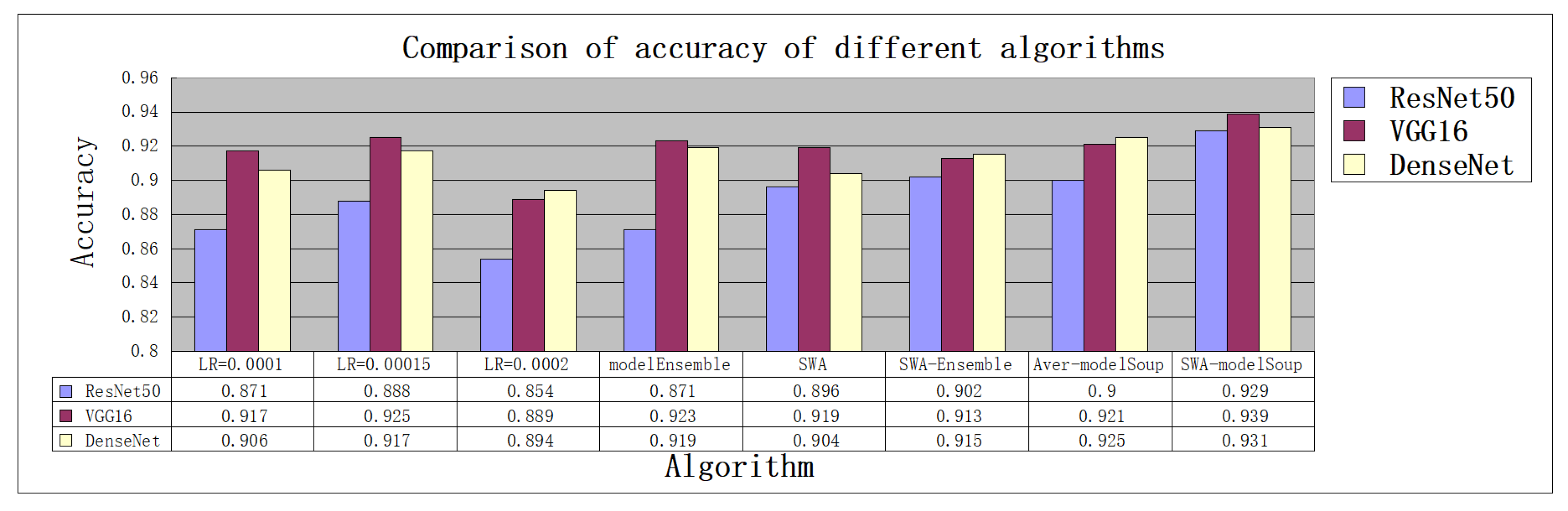
4.3. Evaluation Results

In order to evaluate the effectiveness of the proposed model, measures such as $precision$, $recall$, $accuracy$, and $F1score$ are used. The definitions of $precision$, $recall$, $accuracy$, and $F1score$ are as follows:

$$Precision=\frac{TP}{TP+FP}$$

(12)

$$Recall=\frac{TP}{TP+FN}$$

(13)

$$Accuracy=\frac{TP+TN}{TP+TN+FP+FN}$$

(14)

$$F1score=\frac{2\times recall\times precision}{precision+recall}$$

(15)

where $TP$ is true positive, $TN$ is true negative, $FP$ is false positive, and $FN$ is false negative. Precision refers to the proportion of samples that the model predicts as positive examples and that are actually positive examples. Recall refers to the proportion of samples that are actually positive examples and are correctly predicted as positive examples by the model. The F1 score is the harmonic mean of precision and recall, which is used to comprehensively evaluate the performance of the model on imbalanced datasets. The range of the F1 score is between 0 and 1, the closer to 1, the better the model performance. For a detailed description of these evaluation indicators, please refer to [39].

Table 3. Precision, recall, and F1 score on the SCAN and BreakHis datasets.

Model	Strategy	SCAN			BreakHis
		Precision	Recall	F1 Score	Precision	Recall	F1 Score
ResNet	LR = $0.0001$	$0.888$	$0.871$	$0.880$	$0.952$	$0.950$	$0.950$
	LR = $0.00015$	$0.888$	$0.888$	$0.888$	$0.958$	$0.957$	$0.957$
	LR = $0.0002$	$0.871$	$0.854$	$0.862$	$0.924$	$0.923$	$0.923$
	LR-Ensemble	$0.877$	$0.871$	$0.874$	$0.958$	$0.957$	$0.957$
	LR-Aver-Soup	$0.911$	$0.900$	$0.906$	$0.950$	$0.949$	$0.949$
	CLR-Aver-Soup(SWA)	$0.901$	$0.896$	$0.898$	$0.957$	$0.956$	$0.956$
	CLR-DDWA-Ensemble	$\mathbf{0}.\mathbf{907}$	$\mathbf{0}.\mathbf{902}$	$\mathbf{0}.\mathbf{904}$	$\mathbf{0}.\mathbf{965}$	$\mathbf{0}.\mathbf{963}$	$\mathbf{0}.\mathbf{962}$
	CLR-DDWA-Soup	$\mathbf{0}.\mathbf{929}$	$\mathbf{0}.\mathbf{926}$	$\mathbf{0}.\mathbf{931}$	$\mathbf{0}.\mathbf{979}$	$\mathbf{0}.\mathbf{978}$	$\mathbf{0}.\mathbf{978}$
VGG19-BN	LR = $0.0001$	$0.918$	$0.917$	$0.915$	$0.962$	$0.961$	$0.961$
	LR = $0.00015$	$0.925$	$0.925$	$0.924$	$0.972$	$0.971$	$0.971$
	LR = $0.0002$	$0.892$	$0.889$	$0.887$	$0.963$	$0.961$	$0.961$
	LR-Ensemble	$0.923$	$0.921$	$0.921$	$0.979$	$0.978$	$0.978$
	LR-Aver-Soup	$0.924$	$0.960$	$0.940$	$0.978$	$0.978$	$0.978$
	CLR-Aver-Soup(SWA)	$0.914$	$0.948$	$0.929$	$0.970$	$0.969$	$0.969$
	CLR-DDWA-Ensemble	$\mathbf{0}.\mathbf{915}$	$\mathbf{0}.\mathbf{913}$	$\mathbf{0}.\mathbf{912}$	$\mathbf{0}.\mathbf{979}$	$\mathbf{0}.\mathbf{978}$	$\mathbf{0}.\mathbf{978}$
	CLR-DDWA-Soup	$\mathbf{0}.\mathbf{947}$	$\mathbf{0}.\mathbf{969}$	$\mathbf{0}.\mathbf{958}$	$\mathbf{0}.\mathbf{985}$	$\mathbf{0}.\mathbf{984}$	$\mathbf{0}.\mathbf{984}$
DenseNet	LR = $0.0001$	$0.905$	$0.906$	$0.904$	$0.925$	$0.921$	$0.920$
	LR = $0.00015$	$0.916$	$0.917$	$0.915$	$0.918$	$0.917$	$0.917$
	LR = $0.0002$	$0.893$	$0.894$	$0.892$	$0.926$	$0.922$	$0.921$
	LR-Ensemble	$0.919$	$0.918$	$0.916$	$0.929$	$0.924$	$0.924$
	LR-Aver-Soup	$0.928$	$0.925$	$0.925$	$0.937$	$0.934$	$0.934$
	CLR-Aver-Soup(SWA)	$0.905$	$0.904$	$0.903$	$0.956$	$0.956$	$0.956$
	CLR-DDWA-Ensemble	$\mathbf{0}.\mathbf{916}$	$\mathbf{0}.\mathbf{915}$	$\mathbf{0}.\mathbf{913}$	$\mathbf{0}.\mathbf{960}$	$\mathbf{0}.\mathbf{959}$	$\mathbf{0}.\mathbf{959}$
	CLR-DDWA-Soup	$\mathbf{0}.\mathbf{931}$	$\mathbf{0}.\mathbf{931}$	$\mathbf{0}.\mathbf{931}$	$\mathbf{0}.\mathbf{971}$	$\mathbf{0}.\mathbf{971}$	$\mathbf{0}.\mathbf{971}$

shows the precision, recall, and F1 score of the proposed method, as well as the comparison methods, on the SCAN and BreakHis datasets.

The Model column represents the base model used to generate soup ingredients and the Strategy column represents the strategies used for model training. LR $=0.0001$ represents the results obtained by fine-tuning the model using a constant learning rate of $0.0001$. LR-ensemble represents the majority voting ensemble of models trained with different LRs, i.e., $0.0001$, $0.0015$, and $0.0002$. LR-Aver-Soup represents the average soup model, where its ingredients are models trained using the aforementioned different learning rates. CLR-Aver-Soup (SWA) represents the model obtained using the random weight-averaging method [16]. CLR-DDWA-Ensemble represents the ensemble model, which is obtained by selecting the checkpoint models using CLR through the DDWA strategy. CLR-DDWA-Soup represents the average soup model, which is obtained by selecting the checkpoint models using CLR through the DDWA strategy.

It can be seen from Table 3 that the model obtained by training with different but fixed LR values demonstrates a relatively similar performance across each evaluation index. Ensemble models trained by different LRs can further improve the performance, showing that the models have diversity. LR-Aver-Soup outperforms LR-Ensemble with a precision improvement ratio of $3.9$%. When comparing CLR-Aver-Soup(SWA) and CLR-DDWA-Soup, it can be seen that the latter has better performance, showing the effectiveness of the proposed DDWA ingredient model selection strategy.

Figure 5 shows the confusion matrices of the models based on ResNet.

The values on the diagonal (green) of the confusion matrix indicate the number of correctly classified samples in each class and their proportions relative to the entire dataset. The values in red cells represent the number of misclassified samples and their proportions of the entire dataset. In the last row, the upper value represents the recall of each class. The last column represents the precision corresponding to each class. The most bottom right values represent the accuracy and error rates of the model. It can be seen that the model does not discriminate well between class 1 and class 4 since, for each model, there are samples from class 4 that are misclassified as class 1. Compared with the other models, the CLR-DDWA-Soup model performs better mainly because it has better classification performance in classes 2, 3, and 5, and fewer misclassified samples in class 1 when compared to the other models. Compared with the constant learning rate models, the ensemble-based model (LR-Ensemble) demonstrates a large improvement in the classification accuracy of class 1. We can see that the ensemble model can make good use of the advantages of the three base models. Finally, the CLR-based soup models outperform the models with constant learning rates since their classification performances for class 1 are much better than the other models.

We also provide the top 8 ranking ingredient models as well as their accuracy and diversity values, as shown in

Table 4. Ranking of the ingredient models on the SCAN dataset.

Model	Acc	Div	${\mathbf{Rank}}_{\mathbf{Acc}}$	${\mathbf{Rank}}_{\mathbf{Div}}$	${\mathbf{Rank}}_{\mathbf{Final}}$
model_84	$0.908$	$0.232$	1	1	2
model_51	$0.864$	$0.201$	7	3	10
model_60	$0.880$	$0.157$	2	8	10
model_57	$0.862$	$0.178$	8	5	13
model_27	$0.857$	$0.159$	9	6	15
model_87	$0.872$	$0.129$	4	11	15
model_75	$0.878$	$0.115$	3	12	15
model_30	$0.855$	$0.157$	11	7	18

.

In Table 4 and

Table 5. Ranking of the ingredient models on the BreakHis dataset.

Model	Acc	Div	${\mathbf{Rank}}_{\mathbf{Acc}}$	${\mathbf{Rank}}_{\mathbf{Div}}$	${\mathbf{Rank}}_{\mathbf{Final}}$
model_39	$0.883$	$0.049$	1	1	2
model_42	$0.883$	$0.047$	2	2	4
model_18	$0.867$	$0.044$	4	3	7
model_15	$0.873$	$0.043$	3	4	7
model_27	$0.863$	$0.043$	6	5	11
model_57	$0.865$	$0.041$	5	7	12
model_54	$0.857$	$0.041$	9	8	17
model_24	$0.858$	$0.040$	8	9	17

, the first column represents the names of ingredient models. The second and third columns represent the accuracy and diversity values of each ingredient model, respectively. Moreover, the last three columns represent the ranks of accuracy, diversity, and the final ranking. The final ranking is obtained by simply adding ${\mathbf{Rank}}_{\mathbf{Acc}}$ and ${\mathbf{Rank}}_{\mathbf{Div}}$. We can see from Table 4 that the proposed DDWA method selects ingredient models based on the combination of accuracy and diversity. From the last line of Table 4, it can be seen that even the 11th most accurate ingredient model can be selected by DDWA, which has the advantage of approaching the optimal solution from a wider range.

Figure 6 and Figure 7 show the polylines, representing the accuracies of different models by changing p from $6\%$ to $10\%$ on two datasets. It can be seen that it is not that the more ingredients in the soup, the higher the accuracy; the best classification results can be achieved when the components have the ability to approximate the expected value of the error basin, as depicted in Figure 1.

Figure 8 and Figure 9 show the accuracies of the SCAN and BreakHis datasets for ensemble and soup models based on different ingredient models, i.e., ResNet, VGG, and DenseNet. It can be seen that no single model can achieve the best classification performance in all ingredient models. For CLR-DDWA-Soup, the soup model based on VGG achieves the best performance. The reason may be that the features of the training images in the SCAN dataset are relatively salient and can be effectively extracted via a relatively standard convolutional neural network. In addition, the soup model based on ResNet and DenseNet demonstrates relatively close classification results, which are greatly improved compared to the standard SWA model and the three models with constant learning rates. The highest increase rate reached 8.78%.

Figure 10 shows the receiver operating characteristic (ROC) curves of the models on the BreakHis dataset. It is a curve drawn according to a series of different two-classification methods (cut-off value or determination threshold), with the true positive rate (sensitivity) representing the ordinate and the false positive rate representing the abscissa. The ROC curve can easily determine the ability of a model to recognize samples at a certain threshold. We can see that CLR-DDWA-Soup achieves the largest area under the curve (AUC) among all methods. The larger the AUC, the higher the sensitivity; the lower the misclassification rate, the better the performance of the model.

As indicated by Figure 1, averaging the weights of the ingredient models that are located on the edge of the error basin and that have large diversity can result in a model whose loss is closer to the expected value of the error basin. We interpolate the weights of the two ingredient models to obtain a path through the error basin according to Equation (8). The interpolation parameter $\gamma$ is set to $\{0,\frac{1}{4},\frac{1}{3},\frac{1}{2},\frac{2}{3},\frac{3}{4},1\}$. The accuracy of the model with interpolated weights at each point is recorded, as shown in Figure 11. The x-axis coordinates represent various values of $\gamma$ and the y-axis coordinates represent the model accuracies.

We can see from Figure 11 that for each specific model category (ResNet, VGG, DenseNet), the error variation of the weight interpolation model on the two datasets is always kept within a small fluctuation range, i.e., $\tau \le 0.017$. This result confirms the conclusion that the model selected by the DDWA strategy is located at the edge of the error basin, which shows its effectiveness.

Finally, we present the results of the Friedman test conducted to evaluate the performance of the methods. The Friedman test [40] is a non-parametric test method that uses rank to realize whether there are significant differences in multiple population distributions. The principle hypothesis is that there is no significant difference in multiple population distributions from multiple paired samples. In the field of machine learning, the Friedman test is often used to compare the performances of multiple algorithms, which can verify whether there are significant differences among multiple learning algorithms as a whole.

Let I and J denote the numbers of methods and datasets. In the Friedman test, we first calculate the average accuracy of each algorithm running on different datasets, denoted as $V=\left(v_{ij}\right)$, where $v_{ij}$ represents the accuracy of the ith model on the jth dataset. We then sort $v_{ij}$ in descending order for each dataset and determine the rank values of each algorithm. So far, the Friedman test involves converting the table representing the original experimental results, denoted as $V=\left(v_{ij}\right)$, into the rank table $R=\left(r_{ij}\right)$. In this study, there are 3 base models, 9 methods, and 2 datasets used for the evaluation. We performed the Friedman test on each dataset with different base models. Hence, the size of the ranking matrix R is $(9,3)$, i.e., $I=3\times 9$ and $J=2$. The original hypothesis is that the performances of I different algorithms are similar. The statistic of the Friedman test $F_f$ is defined as follows:

$$F_f=\frac{12\times J}{I\times (I+1)}\left[\sum _{i=1}^I{\overline{R}}_i^2-\frac{I\times {(I+1)}^2}{4}\right]$$

(16)

$F_f$ asymptotically obeys the ${\chi }^2$ distribution with a degree of freedom $I-1$ when $I>5$ and $J>10$. The corresponding value of p is defined as:

$$p=P({\chi }_{I-1}^2\ge F_f)$$

(17)

When the p-value is less than the given significance level $\alpha$, we reject the original hypothesis, meaning that the I algorithms have significant differences in the performance. Otherwise, we accept the original hypothesis, meaning that the I algorithms have no significant differences in performance.

Table 6. Rankings of the models on SCAN and BreakHis in a Friedman test (SCAN/BreakHis/dataset average).

Model	ResNet	VGG	DenseNet	Average
LR = $0.0001$	$23.0$/$17.0$/$20.0$	$9.5$/$10.5$/$10.0$	$13.0$/$23.0$/$18.0$	$16.0$
LR = $0.00015$	$24.0$/$16.0$/$20.0$	$3.5$/$7.0$/$5.25$	$9.5$/$24.0$/$16.75$	$14.0$
LR = $0.0002$	$21.5$/$21.5$/$21.5$	$16.0$/$10.5$/$13.25$	$15.0$/$20.0$/$17.5$	$17.4$
LR-Ensemble	$21.5$/$13.0$/$17.25$	$5.0$/$3.5$/$4.25$	$7.0$/$21.5$/$14.25$	$11.9$
LR-Aver-Soup	$19.0$/$18.0$/$18.5$	$6.0$/$3.5$/$4.75$	$3.5$/$19.0$/$11.25$	$11.5$
CLR-Aver-Soup(SWA)	$18.0$/$14.5$/$16.25$	$8.0$/$8.0$/$8.0$	$14.0$/$14.5$/$14.25$	$12.8$
CLR-DDWA-Ensemble	$20.0$/$9.0$/$14.5$	$12.0$/$3.5$/$7.75$	$11.0$/$12.0$/$11.5$	$11.25$
CLR-DDWA-Soup	$\mathbf{17}.\mathbf{0}$/$\mathbf{3}.\mathbf{5}$/$\mathbf{10}.\mathbf{25}$	$\mathbf{1}.\mathbf{0}$/$\mathbf{1}.\mathbf{0}$/$\mathbf{1}.\mathbf{0}$	$\mathbf{2}.\mathbf{0}$/$\mathbf{6}.\mathbf{0}$/$\mathbf{4}.\mathbf{0}$	$\mathbf{5}.\mathbf{08}$

shows the ranking of the models on both datasets in a Friedman test. There are three values in each cell, representing the average ranking of the method on the SCAN dataset, the average ranking on the BreakHis dataset, and the average ranking of the model on the two datasets. The last column is the total ranking, which is obtained by averaging the rankings on two datasets and three base models. In our study, $I=3\times 9$ and $J=2$, meaning that the values do not meet the requirements of Equation (17). Therefore, it is necessary to look up the table to determine the value of p. Thus, we have $p=0.006$. In the field of machine learning, we usually presuppose that $\alpha$ ranges from $0.05$ to $0.1$. Since the p-value is less than $\alpha$, we need to reject the original hypothesis, which suggests that there are significant differences in the performances among the I algorithms being compared across the datasets.

The smaller the rank value of the model, the better the classification effect. We highlight the smallest rank value in each column in Table 6. It can be seen that the proposed CLR-DDWA-Soup model achieves the best results, which shows its effectiveness.

4.4. Model Complexity

The computational complexity of the proposed model includes three aspects. The first is the computational complexity of training the component models. The component model mainly consists of ResNet50, VGG19, and DenseNet121, and the computational complexity of fine-tuning them is related to the size of the model parameters. Please refer to [34,35,36] for the model parameter information and computational complexity. The second aspect is the computational complexity of ingredient model fusion. For a simple weight-averaging fusion strategy, the weights of each ingredient model are simply averaged. For DDWA, the NDS algorithm needs to be used to sort the ingredient models, resulting in a total computational complexity of $o(nlogn)$, where n is the number of ingredient models to be sorted. The third is the time complexity of inference. Since the model in this paper is a single model after fusion, the computational complexity of inference remains the same as that of a single ingredient model.

5. Discussion

Our rationale for proposing that the model performs well can be attributed to the following factors. On the one hand, during the training of ingredient models, different hyperparameters are fully utilized. Averaging the model weights in different training stages can result in a model that is closer to the optimal solution. On the other hand, using the DDWA model selection strategy to rank and select the ingredient models, we can further improve the performance of the weight fusion model.

Compared to ensemble learning and other model fusion strategies, the proposed model soup has the following advantages. Firstly, in terms of training and inference costs, model soup has certain advantages. In terms of training costs, the training strategy used by model soup is to fine-tune models with different training parameters. Each ingredient model is further trained on a pre-trained model, so the overall training cost is much smaller than starting from scratch. In terms of inference costs, the model soup approach involves averaging, selectively averaging, or weighted averaging the weights of all ingredient models, ultimately resulting in a single model. On the other hand, ensemble learning performs voting or selectively weighting the inference results of n different models, so the inference cost is n times that of model soup. Secondly, in terms of model interpretability, model soup requires the weight structure of the model to be consistent, and its optimal solution estimate is supported by the error basin theory of the loss functions, which has good interpretability. However, for ensemble learning strategies, the component models have different structures and mainly estimate the error bound of the ensemble model through the diversity and accuracy of the component models, so the interpretability is not as good as model soup.

The proposed model has the following limitations. First, the premise of merging ingredient models in the weight space is that the weight structures of each model must be consistent, which limits the diversity of ingredient models, including structural diversity and model type diversity. This kind of model diversity is good at preventing over-fitting during training. Secondly, limited by the error basin minimization theory of the loss function, the model soup proposed in this paper seems to perform better when fine-tuning the pre-training model, and model fine-tuning is easier to satisfy the condition that each component model is located at the edge of the error basin; moreover, the essence of the model soup involves the estimation of the optimal point in the error basin. For ingredient models trained from scratch, the model soup strategy does not lead to significant performance gains. Thirdly, in order to improve the diversity of component models, the model fine-tuning process relies heavily on the adjustment of training parameters, such as CLR, the type and strength of data enhancement, and the optimizer choice, which will increase the training workload and make it challenging to achieve the best training plan.

6. Conclusions

In this paper, we propose a model fusion method in the weight space with a ranking-based model selection strategy. The DDWA strategy selects ingredient models based on accuracy and diversity, causing the selected models to scatter around the edge of the error basin, which makes the weight averaging of the model more efficient. The proposed method can be used in model training or fine-tuning tasks and is especially suitable for medical image classification scenarios with only a small number of training samples. At the same time, compared with ensemble models, our model has lower inference overhead, which is especially suitable for application scenarios with limited computing resources.

Upcoming research will focus on two key areas. The initial aspect will aim to implement the ensemble strategy into the proposed weight fusion model. The second aspect will involve the theoretical derivation of error bounds for the ensemble weight fusion model, considering different strategies.

References

1. Snead, D.R.; Tsang, Y.W.; Meskiri, A.; Kimani, P.K.; Crossman, R.; Rajpoot, N.M.; Blessing, E.; Chen, K.; Gopalakrishnan, K.; Matthews, P.; et al. Validation of digital pathology imaging for primary histopathological diagnosis. Histopathology 2016, 68, 1063–1072. [Google Scholar] [CrossRef] [Green Version]
2. Saltz, J.; Gupta, R.; Hou, L.; Kurc, T.; Singh, P.; Nguyen, V.; Samaras, D.; Shroyer, K.R.; Zhao, T.; Batiste, R.; et al. Spatial organization and molecular correlation of tumor-infiltrating lymphocytes using deep learning on pathology images. Cell Rep. 2018, 23, 181–193. [Google Scholar] [CrossRef] [Green Version]
3. Panayides, A.S.; Amini, A.; Filipovic, N.D.; Sharma, A.; Tsaftaris, S.A.; Young, A.; Foran, D.; Do, N.; Golemati, S.; Kurc, T.; et al. AI in medical imaging informatics: Current challenges and future directions. IEEE J. Biomed. Health Inform. 2020, 24, 1837–1857. [Google Scholar] [CrossRef] [PubMed]
4. LeCun, Y.; Bengio, Y.; Hinton, G. Deep learning. Nature 2015, 521, 436–444. [Google Scholar] [CrossRef]
5. Shinde, P.P.; Shah, S. A review of machine learning and deep learning applications. In Proceedings of the 2018 Fourth International Conference on Computing Communication Control and Automation (ICCUBEA), Pune, India, 16–18 August 2018; pp. 1–6. [Google Scholar]
6. Li, Y.; Huang, C.; Ding, L.; Li, Z.; Pan, Y.; Gao, X. Deep learning in bioinformatics: Introduction, application, and perspective in the big data era. Methods 2019, 166, 4–21. [Google Scholar] [CrossRef] [Green Version]
7. Nichita, A. A Series-Based Deep Learning Approach to Lung Nodule Image Classification. Cancers 2023, 15, 843. [Google Scholar]
8. Deng, J.; Dong, W.; Socher, R.; Li, L.J.; Li, K.; Fei-Fei, L. Imagenet: A large-scale hierarchical image database. In Proceedings of the 2009 IEEE Conference on Computer Vision and Pattern Recognition, Miami, FL, USA, 20–25 June 2009; pp. 248–255. [Google Scholar]
9. Dai, Z.; Liu, H.; Le, Q.V.; Tan, M. CoAtNet: Marrying Convolution and Attention for All Data Sizes. arXiv 2021, arXiv:2106.04803. [Google Scholar]
10. Hu, L.S.; Yoon, H.; Eschbacher, J.M.; Baxter, L.C.; Dueck, A.C.; Nespodzany, A.; Smith, K.A.; Nakaji, P.; Xu, Y.; Wang, L.; et al. Accurate patient-specific machine learning models of glioblastoma invasion using transfer learning. Am. J. Neuroradiol. 2019, 40, 418–425. [Google Scholar] [CrossRef]
11. Sheehan, S.; Mawe, S.; Cianciolo, R.E.; Korstanje, R.; Mahoney, J.M. Detection and classification of novel renal histologic phenotypes using deep neural networks. Am. J. Pathol. 2019, 189, 1786–1796. [Google Scholar] [CrossRef]
12. Roster, K.; Connaughton, C.; Rodrigues, F.A. Forecasting new diseases in low-datasettings using transfer learning. arXiv 2022, arXiv:2204.05059. [Google Scholar]
13. Han, W.; Johnson, C.; Gaed, M.; Gómez, J.A.; Moussa, M.; Chin, J.L.; Pautler, S.; Bauman, G.S.; Ward, A.D. Histologic tissue components provide major cues for machine learning-based prostate cancer detection and grading on prostatectomy specimens. Sci. Rep. 2020, 10, 9911. [Google Scholar] [CrossRef]
14. Hassan, S.A.; Sayed, M.S.; Abdalla, M.I.; Rashwan, M.A. Breast cancer masses classification using deep convolutional neural networks and transfer learning. Multimed. Tools Appl. 2020, 79, 30735–30768. [Google Scholar] [CrossRef]
15. Liu, W.; Mo, J.; Zhong, F. Class Imbalanced Medical Image Classification Based on Semi-Supervised Federated Learning. Appl. Sci. 2023, 13, 2109. [Google Scholar] [CrossRef]
16. Izmailov, P.; Podoprikhin, D.; Garipov, T.; Vetrov, D.; Wilson, A.G. Averaging weights leads to wider optima and better generalization. arXiv 2018, arXiv:1803.05407. [Google Scholar]
17. Wortsman, M.; Ilharco, G.; Gadre, S.Y.; Roelofs, R.; Gontijo-Lopes, R.; Morcos, A.S.; Namkoong, H.; Farhadi, A.; Carmon, Y.; Kornblith, S.; et al. Model soups: Averaging weights of multiple fine-tuned models improves accuracy without increasing inference time. arXiv 2022, arXiv:2203.05482. [Google Scholar]
18. Choshen, L.; Venezian, E.; Slonim, N.; Katz, Y. Fusing finetuned models for better pretraining. arXiv 2022, arXiv:2204.03044. [Google Scholar]
19. Dansereau, C.; Sobral, M.; Bhogal, M.; Zalai, M. Model soups to increase inference without increasing compute time. arXiv 2023, arXiv:2301.10092. [Google Scholar]
20. Draxler, F.; Veschgini, K.; Salmhofer, M.; Hamprecht, F. Essentially no barriers in neural network energy landscape. In Proceedings of the 35th International Conference on Machine Learning, Stockholm, Sweden, 10–15 July 2018. [Google Scholar]
21. Smith, L.N. Cyclical learning rates for training neural networks. In Proceedings of the 2017 IEEE Winter Conference on Applications of Computer Vision (WACV), Santa Rosa, CA, USA, 24–31 March 2017. [Google Scholar]
22. Wei, L.; Wan, S.; Guo, J.; Wong, K.K. A novel hierarchical selective ensemble classifier with bioinformatics application. Artif. Intell. Med. 2017, 83, 82–90. [Google Scholar] [CrossRef]
23. Smith, L.N.; Topin, N. Exploring loss function topology with cyclical learning rates. arXiv 2017, arXiv:1702.04283. [Google Scholar]
24. Garipov, T.; Izmailov, P.; Podoprikhin, D.; Vetrov, D.P.; Wilson, A.G. Loss Surfaces, Mode Connectivity, and Fast Ensembling of DNNs. In Proceedings of the Advances in Neural Information Processing Systems 31 (NeurIPS 2018), Montreal, QC, Canada, 3–8 December 2018. [Google Scholar]
25. Jain, P.; Kakade, S.M.; Kidambi, R.; Netrapalli, P.; Sidford, A. Parallelizing Stochastic Gradient Descent for Least Squares Regression: Mini-batching, Averaging, and Model Misspecification. J. Mach. Learn. Res. 2018, 18, 1–42. [Google Scholar]
26. Guo, H.; Jin, J.; Liu, B. Stochastic Weight Averaging Revisited. Appl. Sci. 2023, 13, 2935. [Google Scholar] [CrossRef]
27. Neyshabur, B.; Sedghi, H.; Zhang, C. What is being transferred in transfer learning? Adv. Neural Inf. Process. Syst. 2020, 33, 512–523. [Google Scholar]
28. Hameed, Z.; Zahia, S.; Garcia-Zapirain, B.; Javier Aguirre, J.; María Vanegas, A. Breast cancer histopathology image classification using an ensemble of deep learning models. Sensors 2020, 20, 4373. [Google Scholar] [CrossRef] [PubMed]
29. Sohail, A.; Khan, A.; Nisar, H.; Tabassum, S.; Zameer, A. Mitotic nuclei analysis in breast cancer histopathology images using deep ensemble classifier. Med. Image Anal. 2021, 72, 102121. [Google Scholar] [CrossRef]
30. Kumar, D.; Batra, U. Classification of Invasive Ductal Carcinoma from histopathology breast cancer images using Stacked Generalized Ensemble. J. Intell. Fuzzy Syst. 2021, 40, 4919–4934. [Google Scholar] [CrossRef]
31. Ahuja, S.; Panigrahi, B.K.; Dey, N.; Rajinikanth, V.; Gandhi, T.K. Deep transfer learning-based automated detection of COVID-19 from lung CT scan slices. Appl. Intell. 2021, 51, 571–585. [Google Scholar] [CrossRef] [PubMed]
32. Lawton, S.; Viriri, S. Detection of COVID-19 from CT Lung Scans Using Transfer Learning. Comput. Intell. Neurosci. 2021, 2021, 5527923. [Google Scholar] [CrossRef]
33. Jangam, E.; Barreto, A.A.D.; Annavarapu, C.S.R. Automatic detection of COVID-19 from chest CT scan and chest X-Rays images using deep learning, transfer learning and stacking. Appl. Intell. 2022, 52, 2243–2259. [Google Scholar] [CrossRef]
34. He, K.; Zhang, X.; Ren, S.; Sun, J. Deep residual learning for image recognition. In Proceedings of the IEEE Conference on Computer Vision and Pattern Recognition, Las Vegas, NV, USA, 27–30 June 2016; pp. 770–778. [Google Scholar]
35. Simonyan, K.; Zisserman, A. Very deep convolutional networks for large-scale image recognition. arXiv 2014, arXiv:1409.1556. [Google Scholar]
36. Huang, G.; Liu, Z.; van der Maaten, L.; Weinberger, K.Q. Densenet: Densely connected convolutional networks. In Proceedings of the IEEE Computer Society Conference on Computer Vision and Pattern Recognition, Honolulu, HI, USA, 21–26 July 2017; Volume 30, pp. 82–84. [Google Scholar]
37. Cubuk, E.D.; Zoph, B.; Shlens, J.; Le, Q.V. RandAugment: Practical automated data augmentation with a reduced search space. In Proceedings of the IEEE/CVF Conference on Computer Vision and Pattern Recognition Workshops, Seattle, WA, USA, 14–19 June 2020; pp. 702–703. [Google Scholar]
38. Lu, Z.; Wu, X.; Zhu, X.; Bongard, J. Ensemble pruning via individual contribution ordering. In Proceedings of the 16th ACM SIGKDD International Conference on Knowledge Discovery and Data Mining, Washington, DC, USA, 25–28 July 2010; pp. 871–880. [Google Scholar]
39. Sahu, A.K.; Sahu, M.; Patro, P.; Sahu, G.; Nayak, S.R. Dual image-based reversible fragile watermarking scheme for tamper detection and localization. Pattern Anal. Appl. 2023, 26, 571–590. [Google Scholar] [CrossRef]
40. Demiar, J.; Schuurmans, D. Statistical Comparisons of Classifiers over Multiple Data Sets. J. Mach. Learn. Res. 2006, 7, 1–30. [Google Scholar]
Figure 1. Two cases of weight averaging of soup ingredients.
Applsci 13 07009 g001
Figure 2. Main steps of the proposed model.
Applsci 13 07009 g002
Figure 3. Two examples of the SCAN dataset.
Applsci 13 07009 g003
Figure 4. Two examples of the BreakHis dataset.
Applsci 13 07009 g004
Figure 5. Confusion matrix of the models based on ResNet. (a) CLR-Aver-Soup (SWA); (b) CLR-DDWA-Ensemble; (c) CLR-DDWA-Soup; (d) LR = 0.0001 ; (e) LR = 0.00015 ; (f) LR = 0.0002 ; (g) LR-Aver-Soup; (h) LR-Ensemble.
Applsci 13 07009 g005
Figure 6. The accuracy of the polyline representing CLR-DDWA-Soup, fusing the top p% ingredient models on the SCAN dataset.
Applsci 13 07009 g006
Figure 7. The accuracy of the polyline representing CLR-DDWA-Soup, fusing the top p% ingredient models on the BreakHis dataset.
Applsci 13 07009 g007
Figure 8. Accuracies of different models on the SCAN dataset.
Applsci 13 07009 g008
Figure 9. Accuracies of different models on the BreakHis dataset.
Applsci 13 07009 g009
Figure 10. ROC curves of the models on the BreakHis dataset.
Applsci 13 07009 g010
Figure 11. Model losses with interpolated weights on the SCAN and BreakHis datasets.
Applsci 13 07009 g011