
Tensile Stress Evolution Outside Deformation Zone of Cold Rolled Strip
Abstract
:1. Introduction
2. Governing Equations
2.1. Problem Description
2.2. Solution Technique
3. Results Analysis
4. Discussion
5. Experiment
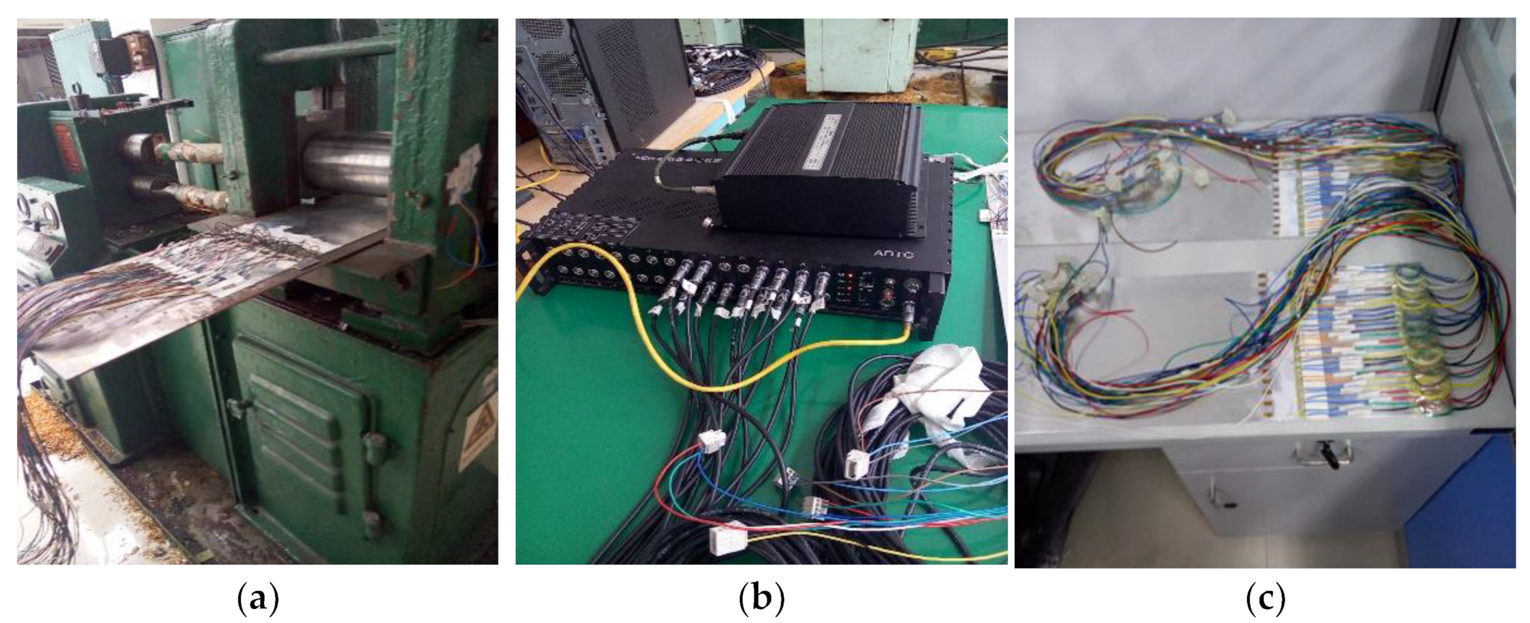
5.1. Experimental Equipment and Materials
5.2. Experimental Results
5.3. Analysis
6. Conclusions
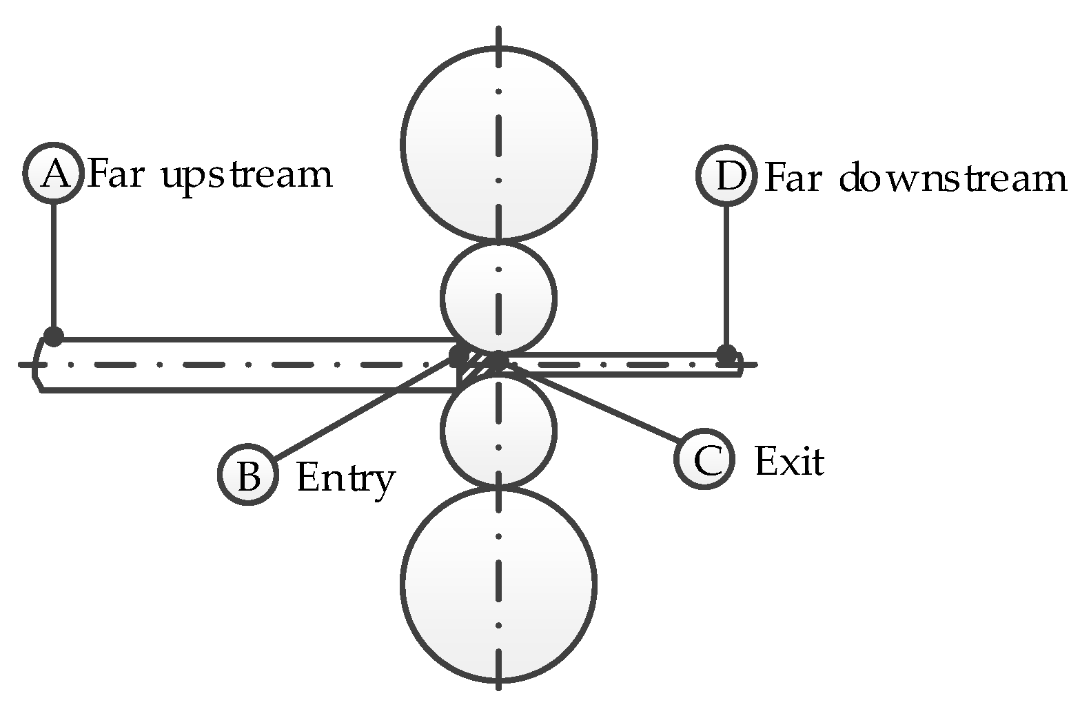
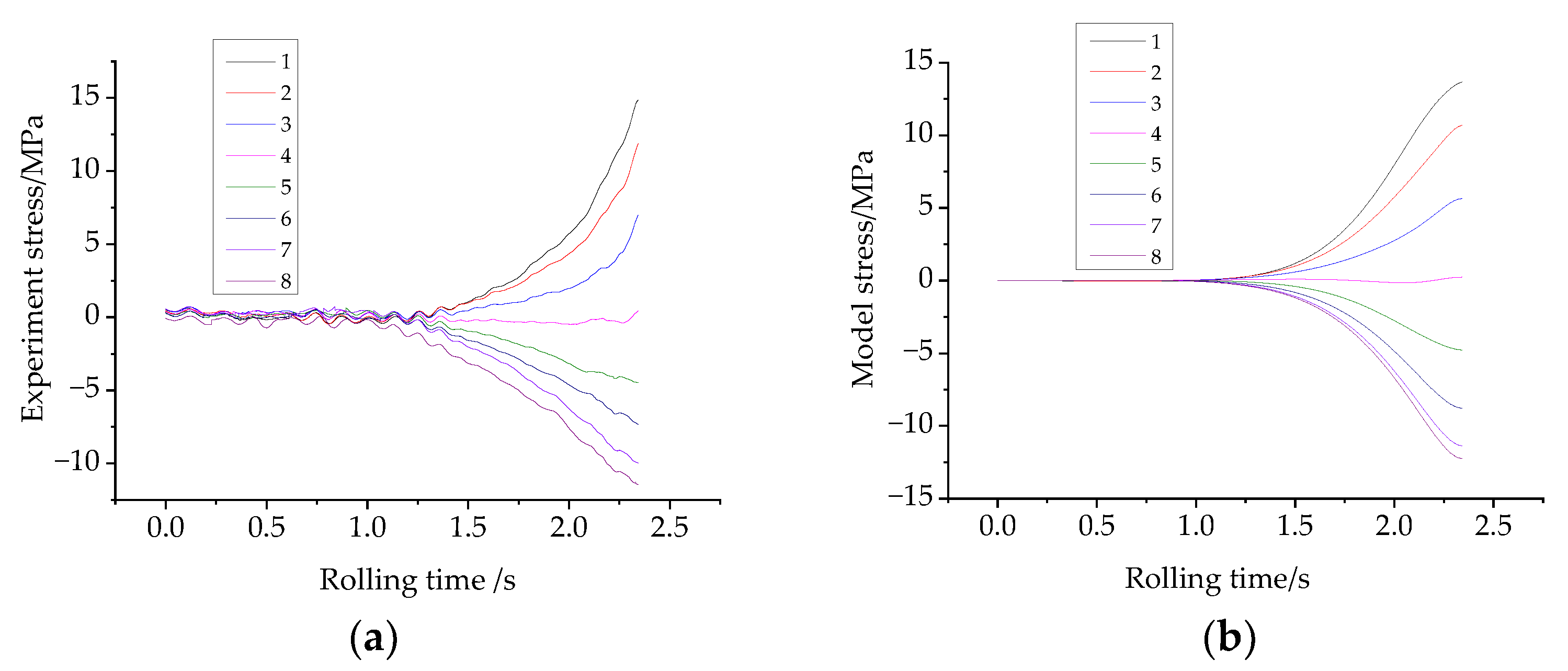
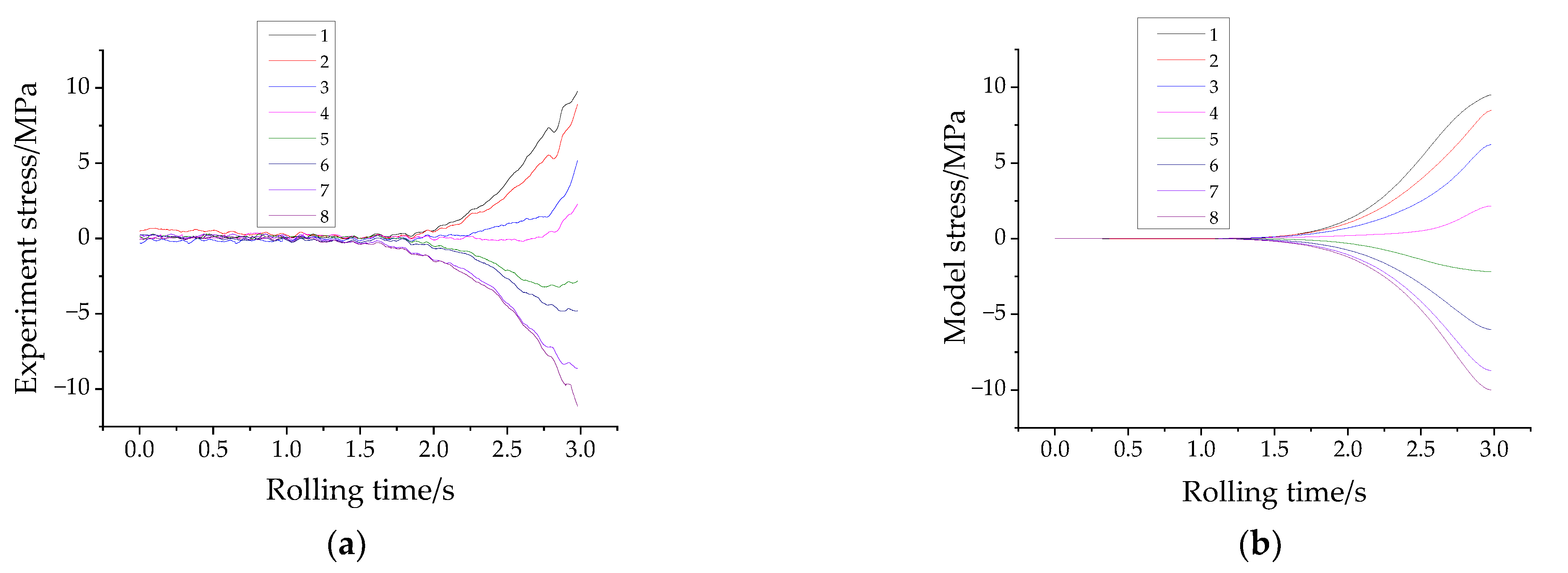
- The theoretical and experimental results show that the tensile stress distribution in the upstream and downstream regions of the deformation zone is different from that in the entry and exit regions of the deformation zone. Specially, between the exit of the deformation zone and the downstream region, the velocity distribution gradually becomes more uniform, while the tensile stress distribution gradually stabilizes.
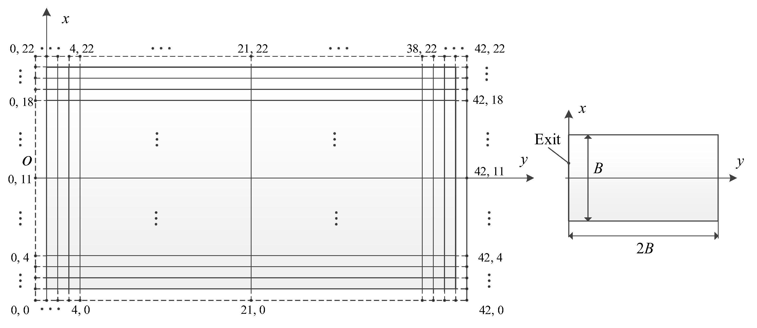
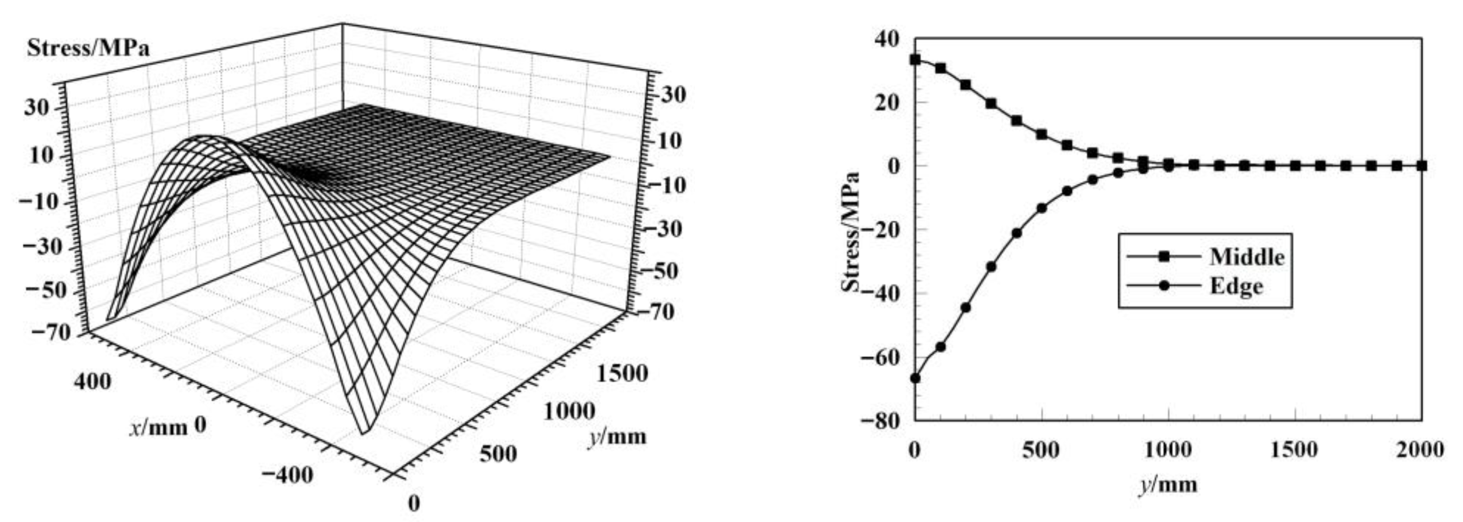
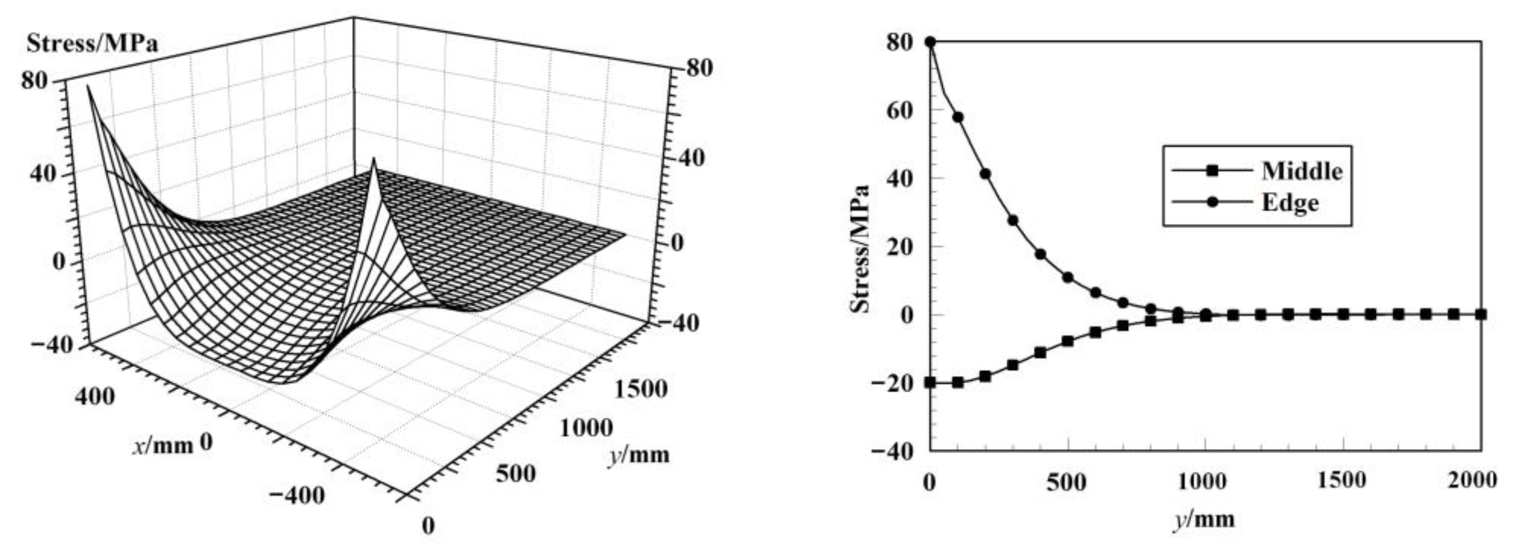
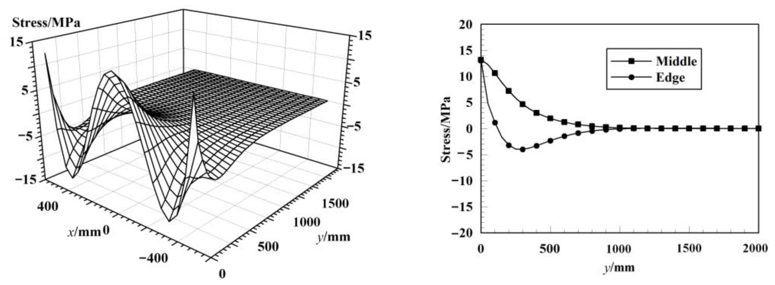
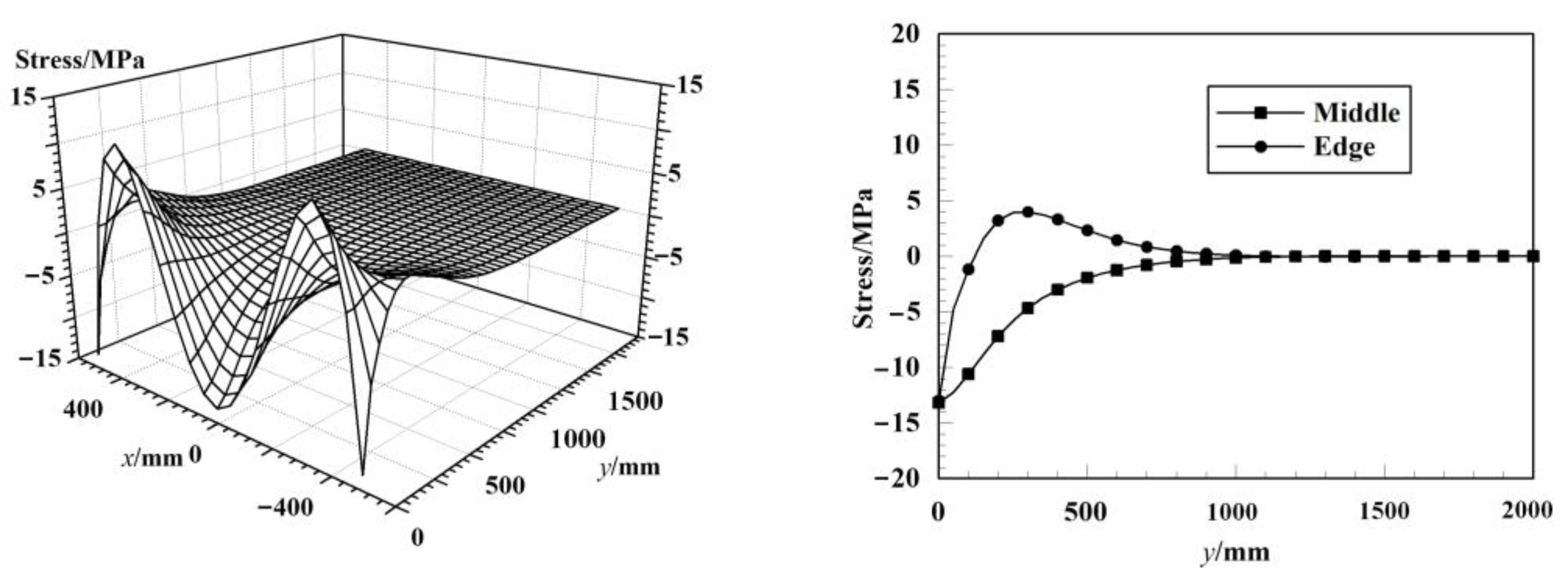
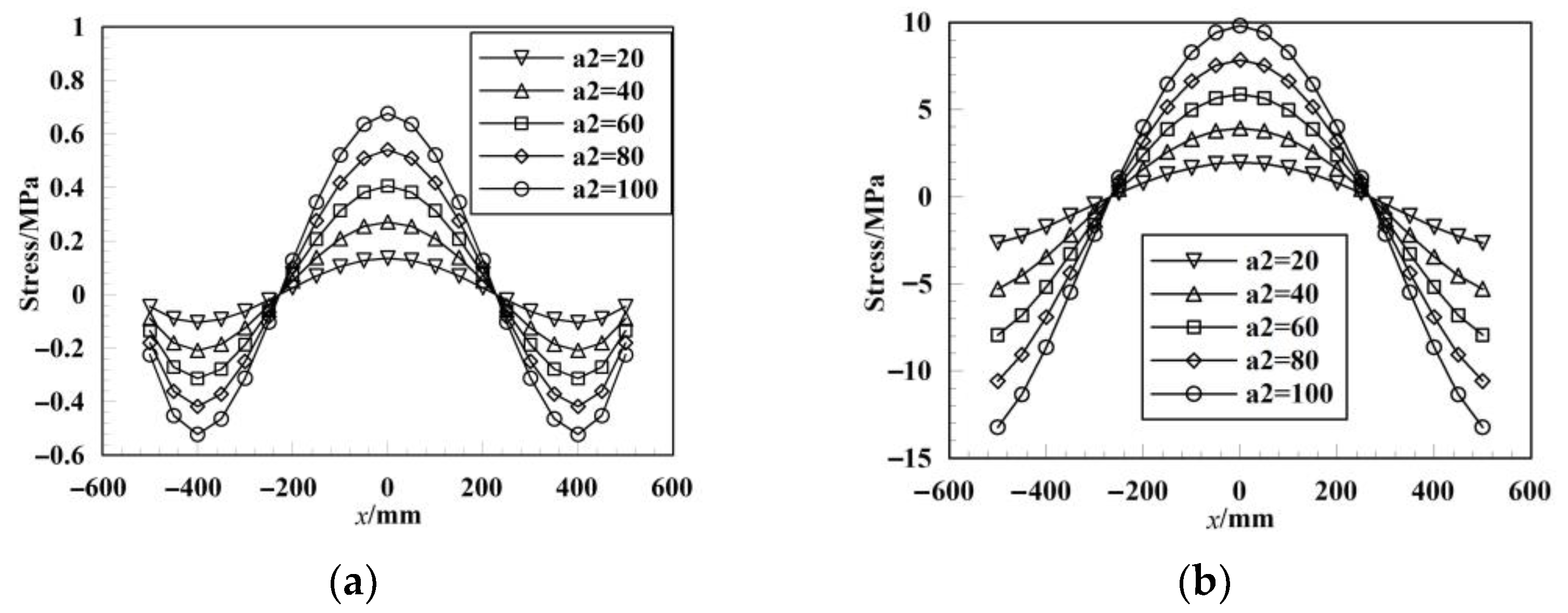
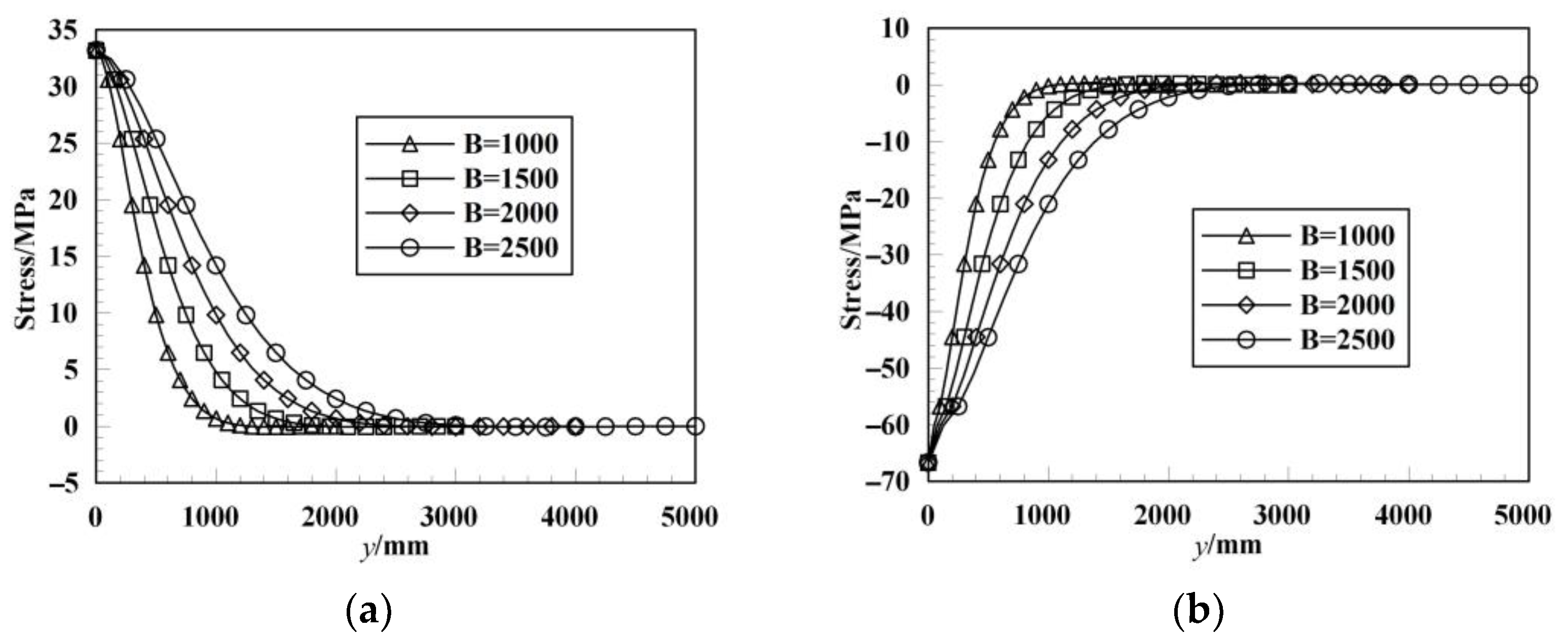
- The tension stress fluctuation of the strip outside the deformation zone can be regarded as a plane stress problem. A basic differential equation can be established based on the stress function method, and the finite difference method can be used to solve the differential equation. The calculated results indicate that the stress amplitude at different distances from the exit has a linear relationship with the amplitude of the initial stress, which falls roughly 98.8% after a distance of one strip width. The initial stress amplitude and strip width have little effect on the change trend of the stress evolution caused by the uneven velocity distribution, and the initial stress form is influential. The initial stress form can be broken down into two basic modes, that is, a quadratic or quartic coefficient. Any type of initial stress form can be considered as a linear combination of the two basic modes.
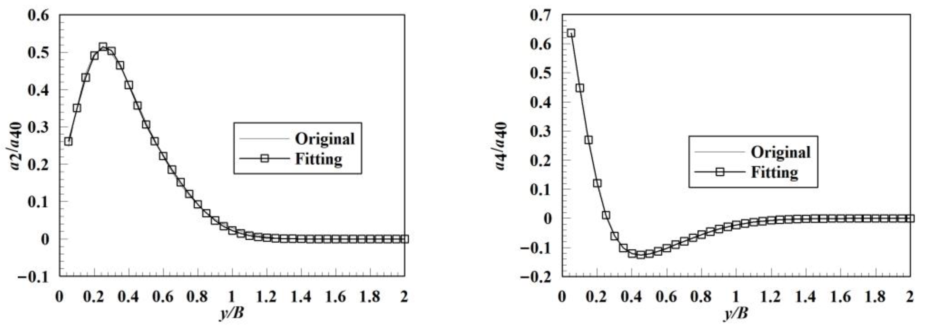
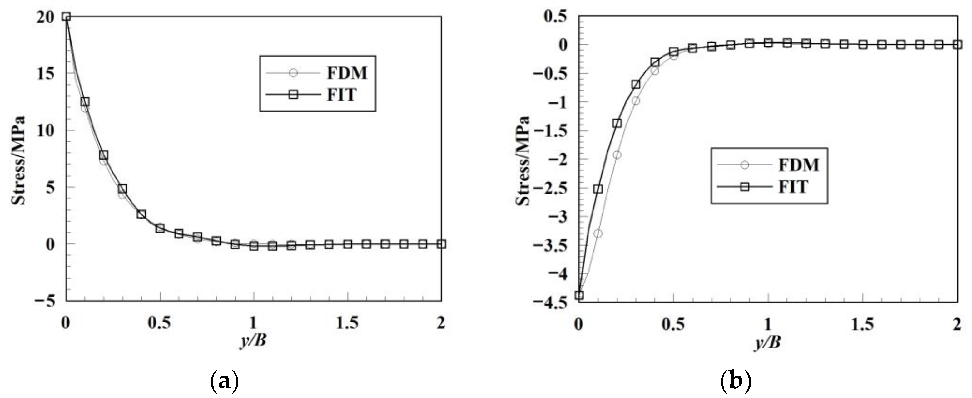
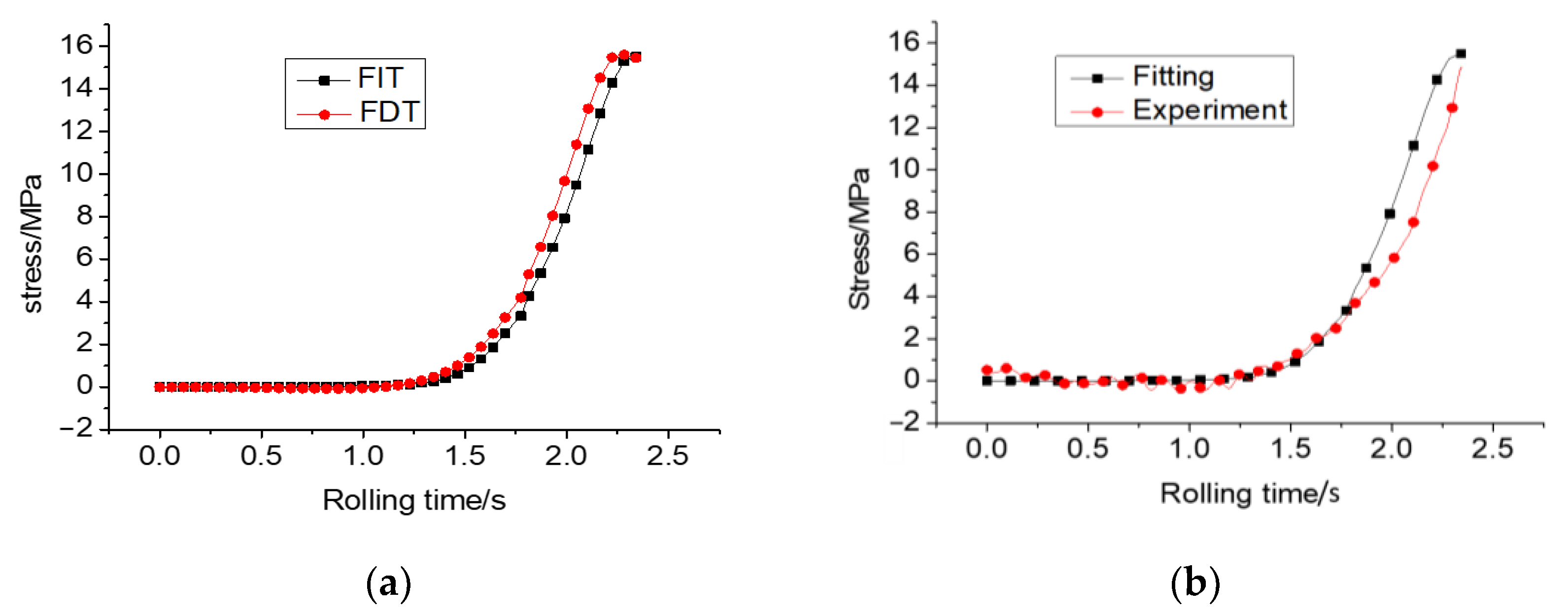
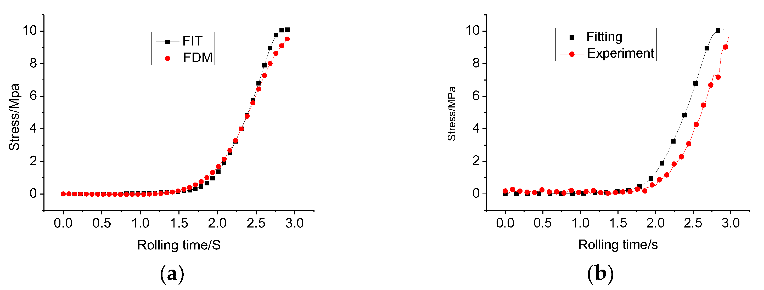
- To save time, a “Gaussian” curve is proposed to fit the calculated results of the finite difference method. The simulation results reveal that the stress evolution calculated by the fitting equation is in good agreement with that calculated by the finite difference method.
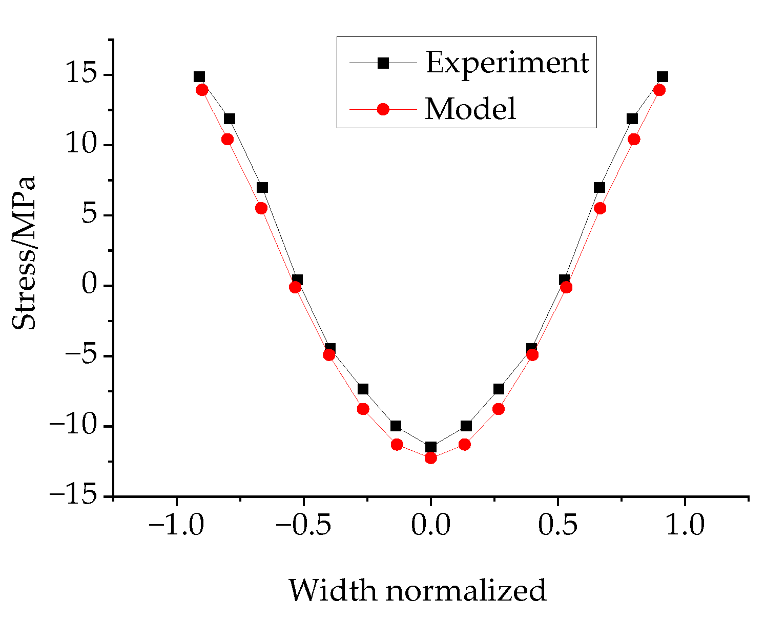
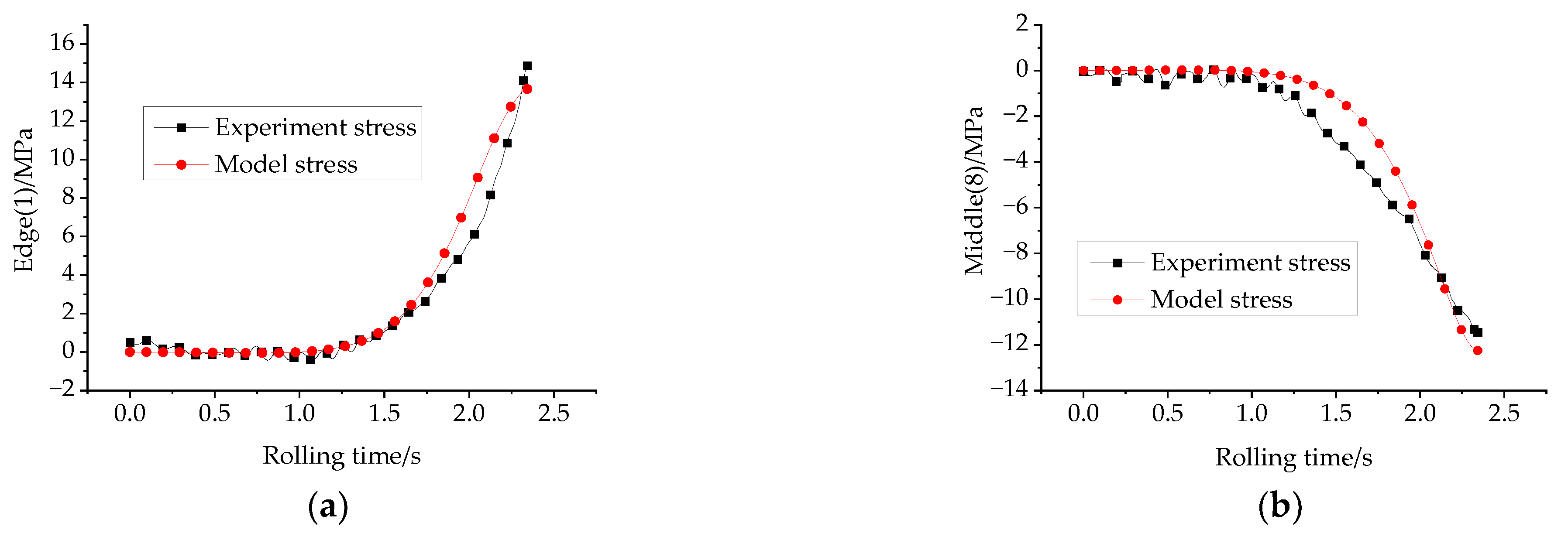
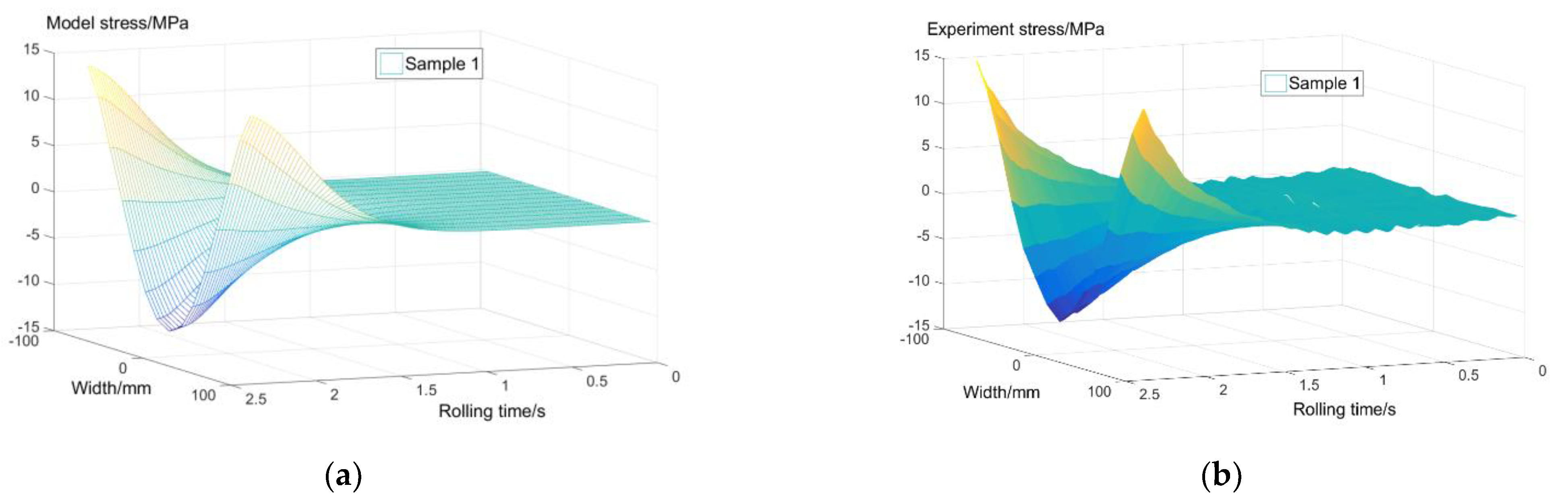
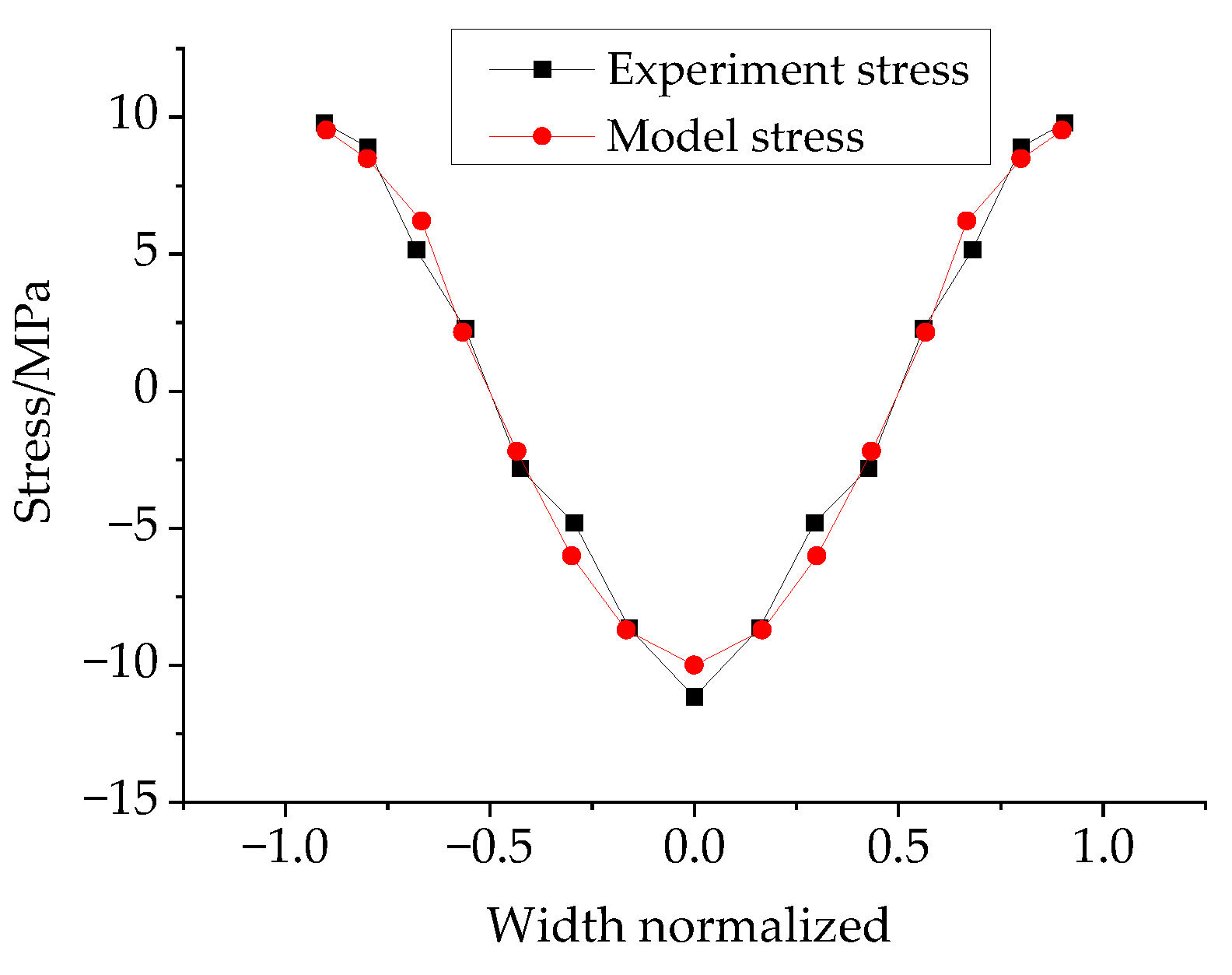
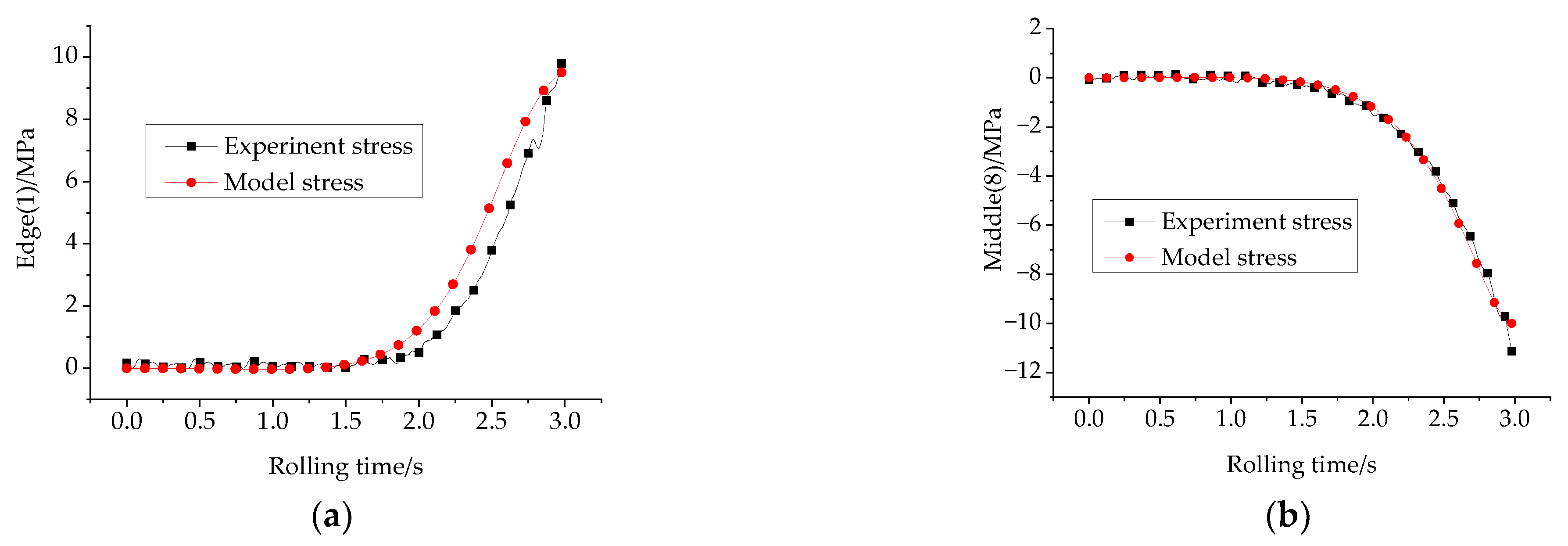
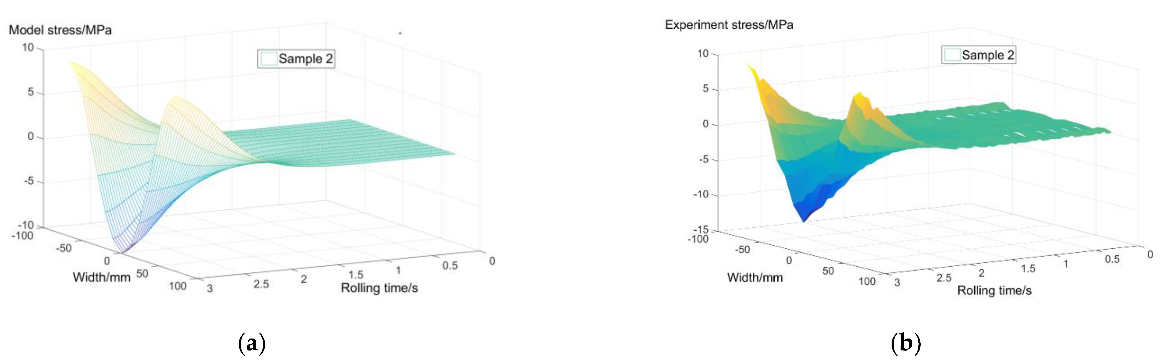
- To verify the practicability of the proposed model, a tensile stress rheology experiment is conducted, as shown above, and it can be seen that the experimental results fit well with the model results. Thus, it can be concluded that the model is correct and practical. The comparison of the fitting results with the model results and experimental results reveals that the proposed “Gaussian” curve is accurate and practical.
Author Contributions
Funding
Institutional Review Board Statement
Informed Consent Statement
Data Availability Statement
Acknowledgments
Conflicts of Interest
References
- Sun, J.; Shan, P.F.; Wei, Z.; Hu, Y.H.; Wang, Q.L.; Peng, W.; Zhang, D.H. Data-based flatness prediction and optimization in tandem cold rolling. J. Iron Steel Res. Int. 2020, 28, 563–573. [Google Scholar] [CrossRef]
- Wang, Y.S.; Xu, X.D.; Ren, B.B.; Liu, J.; Zhao, R.G. Effect of Geometrical Factors on Torsion in Cold Roll Forming of the Lower Side Beam of a Car. Appl. Sci. 2021, 11, 7852. [Google Scholar] [CrossRef]
- Roh, Y.H.; Byon, S.M.; Lee, Y. Numerical Analysis of Edge Cracking in High-Silicon Steel during Cold Rolling with 3D Fracture Locus. Appl. Sci. 2021, 11, 8408. [Google Scholar] [CrossRef]
- Xu, D.; Yang, Q.; Wang, X.C.; He, H.; Sun, Y.Z.; Li, W.P. An Experimental Investigation of Steel Surface Topography Transfer by Cold Rolling. Micromachines 2020, 11, 916. [Google Scholar] [CrossRef] [PubMed]
- Wang, D.C.; Liu, H.M.; Liu, J. Research and Development Trend of Shape Control for Cold Rolling Strip. Chin. J. Mech. Eng. 2017, 30, 1248–1261. [Google Scholar] [CrossRef] [Green Version]
- Yi, G.D.; Liang, Y.; Wang, C.; Xu, J.H. Evolution of Residual Stress Based on Curvature Coupling in Multi-Roll Levelling. Appl. Sci. 2019, 9, 4975. [Google Scholar] [CrossRef] [Green Version]
- Shohet, K.N.; Townsend, N.A. Roll Bending Methods of Crown Control in Four-High Plate Mills. J. Iron Steel Inst. 1968, 11, 1088–1098. [Google Scholar]
- Jiang, G.Y.; Wang, Y.Q.; Yan, X.C. Analysis on solution of residual stress for cold rolling strip. J. Iron Steel Res. 2010, 22, 16–18. [Google Scholar]
- Xu, L.J. Flatness Control in Cold Strip Rolling and Mill Type Selection; Metallurgical Industry Press: Beijing, China, 2007. [Google Scholar]
- Matsumoto, H. 2-Dimensional lateral-material-flow model reduced from 3-Dimensional theory for flat rolling. ISIJ Int. 1991, 31, 550–558. [Google Scholar] [CrossRef]
- Kim, Y.K.; Kwak, W.J.; Shin, T.J.; Hwang, S.M. A new model for the prediction of roll force and tension profiles in flat rolling. ISIJ Int. 2010, 50, 1644–1652. [Google Scholar] [CrossRef] [Green Version]
- Bryant, G.F. Automation of Tandem Mills; The Iron and Steel Institute: London, UK, 1973; pp. 176–212. [Google Scholar]
- Ishikawa, T.; Tozawa, Y.; Yukawa, N.; Yamanaka, M. Analytical Approach to the Shape of Rolled Strip. In Advanced Technology of Plasticity; Springer: Berlin/Heidelberg, Germany, 1984; pp. 1161–1166. [Google Scholar]
- Liu, X.H.; Jiang, Z.Y.; Wang, G.D. Analysis of 3-D Deformation for Crowning Strip Rolling by Rigid-Plastic FEM. In Advanced Technology of Plasticity; Springer: Berlin/Heidelberg, Germany, 1993; pp. 717–720. [Google Scholar]
- Wang, D.C.; Liu, H.M. A model coupling method for shape prediction. J. Iron Steel Res. Int. 2012, 19, 22–27. [Google Scholar] [CrossRef]
- Lian, J.C. Analysis of profile and shape control in flat rolling. In Proceedings of the First International Conference on Steel Rolling, Tokyo, Japan, 29 September–4 October 1980; The Iron and Steel Institute of Japan: Tokyo, Japan, 1980; Volume 2, pp. 713–720. [Google Scholar]
- Liu, H.M.; Chen, S.W.; Peng, Y.; Sun, J.L. Strip layer method for analysis of the three-dimensional stresses and spread of large cylindrical shell rolling. Chin. J. Mech. Eng. 2015, 28, 556–564. [Google Scholar] [CrossRef]
- Liu, H.M.; Lian, J.C.; Duan, Z.Y. Study on the transverse distributions of front and back tensions in strip rolled 4-high mill. Heavy Mach. 1989, 4, 12–20. [Google Scholar]
- Liu, H.M. Three Dimensional Rolling Theory and Application; Science Press: Beijing, China, 1999; pp. 1–53, 276–283. [Google Scholar]
- Ishikawa, T.; Nakamura, M.; Tozawa, Y. Three-dimensional analysis of sheet rolling considering roll deformation. Plast. Process. 1980, 21, 902–908. [Google Scholar]
- Cresdee, R.B.; Wdwards, W.J.; Thomas, P.J. An advanced model for flatness and profile prediction in hot rolling. Iron Steel Eng. 1991, 68, 41–45. [Google Scholar]
- Yuen, W.Y.; Cozijnsen, M. Strip Shape Analysis in Cold Rolling. In Proceedings of the 44th Mechanical Working and Steel Processing Conference Proceedings, Orlando, FL, USA, 8–11 September 2002. [Google Scholar]
- Tarnoplskaya, T.F.; Hoog, R.D. An efficient method for strip flatness analysis in cold rolling. Math. Eng. Ind. 1998, 7, 71–95. [Google Scholar]
- Cao, H.D. Plastic Deformation Mechanics Basis and Rolling Theory; Mechanical Industry Press: Beijing, China, 1981; pp. 151–159. [Google Scholar]
- Domanti, S.; Mcelwain, D.S.; Middleton, R.H.; Edwards, W.J. The decay of stresses induced by flat rolling of metal strip. Int. J. Mech. Sci. 1993, 35, 897–907. [Google Scholar] [CrossRef]
- Li, W.T.; Huang, B.H.; Bi, Z.B. Analysis and Application of Thermal Stress Theory; China Electric Power Press: Beijing, China, 2006; pp. 115–128. [Google Scholar]
- Wang, D.C. Entry and exit stress variation of cold rolling strip. J. Iron Steel Res. Int. 2012, 19, 19–24. [Google Scholar] [CrossRef]


| Mode | A1 | B1 | C1 | A2 | B2 | C2 | |
|---|---|---|---|---|---|---|---|
| 1 | a2 | 0.01292 | 0.03105 | 0.02057 | 1.114 | −0.1145 | 0.6015 |
| a4 | −0.07125 | 0.3252 | 0.2516 | −0.119 | 0.431 | 0.4751 | |
| 2 | a2 | 0.3064 | 0.2181 | 0.2123 | 0.2661 | 0.4202 | 0.3696 |
| a4 | 1.059 | −0.0938 | 0.2506 | −0.1504 | 0.2766 | 0.5254 | |
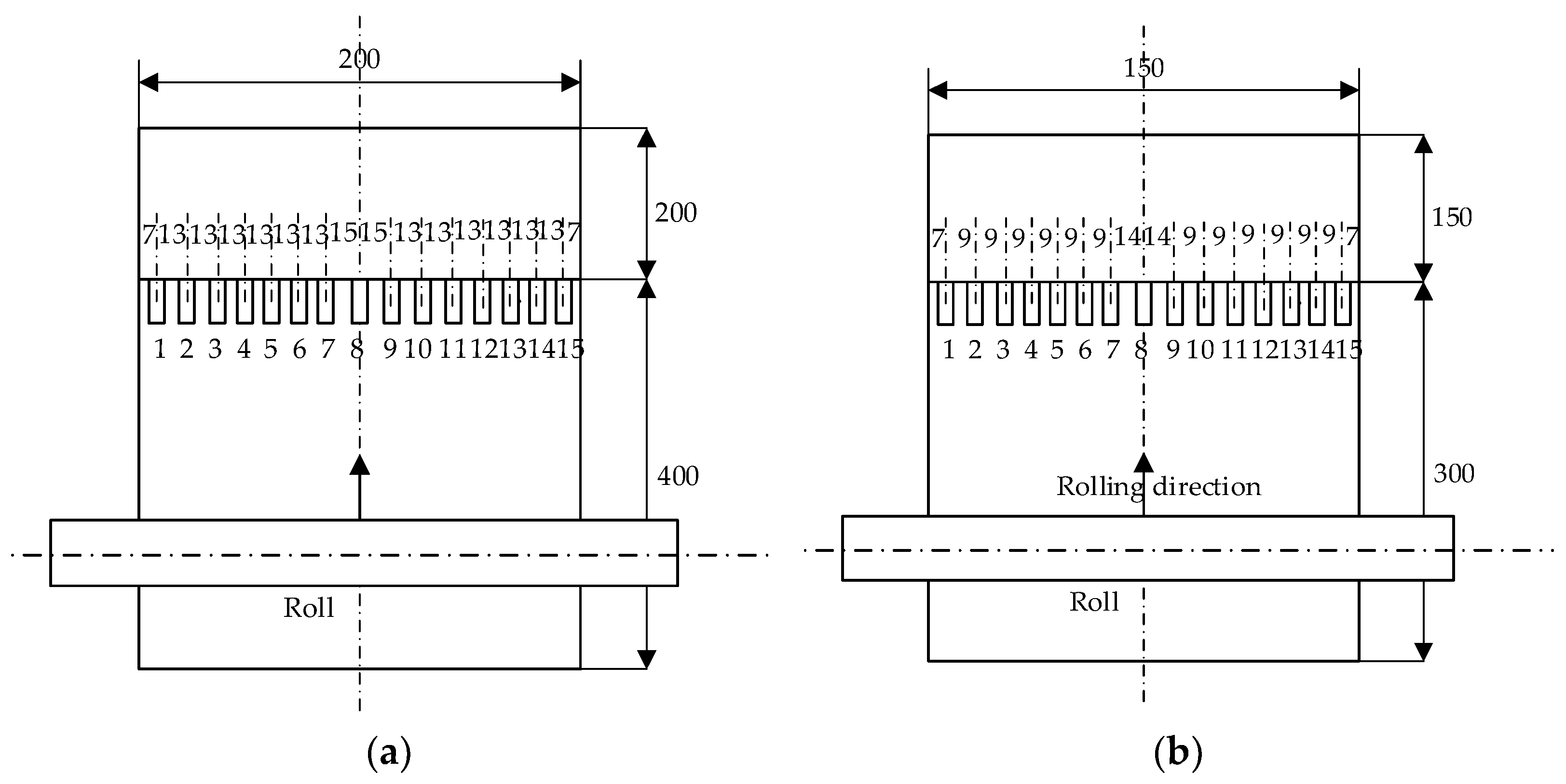
| Sample Number | The Initial Specification | |||
|---|---|---|---|---|
| Length/mm | Rolling Length/mm | Width/mm | Thickness/mm | |
| 1 | 600 | 400 | 200 | 1.7 |
| 2 | 450 | 300 | 150 | 1.7 |
Disclaimer/Publisher’s Note: The statements, opinions and data contained in all publications are solely those of the individual author(s) and contributor(s) and not of MDPI and/or the editor(s). MDPI and/or the editor(s) disclaim responsibility for any injury to people or property resulting from any ideas, methods, instructions or products referred to in the content. |
© 2023 by the authors. Licensee MDPI, Basel, Switzerland. This article is an open access article distributed under the terms and conditions of the Creative Commons Attribution (CC BY) license (https://creativecommons.org/licenses/by/4.0/).
Share and Cite
Zhang, K.; Wang, D.; Xu, Y.; Liu, H. Tensile Stress Evolution Outside Deformation Zone of Cold Rolled Strip. Appl. Sci. 2023, 13, 6781. https://doi.org/10.3390/app13116781
Zhang K, Wang D, Xu Y, Liu H. Tensile Stress Evolution Outside Deformation Zone of Cold Rolled Strip. Applied Sciences. 2023; 13(11):6781. https://doi.org/10.3390/app13116781
Chicago/Turabian StyleZhang, Kangwu, Dongcheng Wang, Yanghuan Xu, and Hongmin Liu. 2023. "Tensile Stress Evolution Outside Deformation Zone of Cold Rolled Strip" Applied Sciences 13, no. 11: 6781. https://doi.org/10.3390/app13116781