Portrait Reification with Generative Diffusion Models

Abstract

An application of Generative Diffusion Techniques for the reification of human portraits in artistic paintings is presented. By reification we intend the transformation of the painter’s figurative abstraction into a real human face. The application exploits a recent embedding technique for Denoising Diffusion Implicit Models (DDIM), inverting the generative process and mapping the visible image into its latent representation. In this way, we can first embed the portrait into the latent space, and then use the reverse diffusion model, trained to generate real human faces, to produce the most likely real approximation of the portrait. The actual deployment of the application involves several additional techniques, mostly aimed to automatically identify, align, and crop the relevant portion of the face, and to postprocess the generated reification in order to enhance its quality and to allow a smooth reinsertion in the original painting.

1. Introduction

Have you ever wondered what could have been the actual appearance of some famous historical figure, according to the portraits we have of her/him? Are you curious to see how Vermer’s famous girl with a pearl earring may have actually looked? With the help of diffusion generative models and the reification application described in this article, this is now possible.

The key ingredient of the reification process is the embedding procedure recently explored in [1], permitting the computation of the latent representation of an image by means of a suitably trained neural network. This embedding network provides, in the case of diffusion models, a functionality essentially equivalent to re-coders for Generative Adversarial Networks (GANs) [2,3] or to encoders in the case of Variational Autoencoders (VAEs) [4,5].

If the generator has been trained to sample real human faces, starting from the embedding of the portrait, we shall be able to reconstruct the most likely real approximation of the original subject. This is particularly effective for reverse diffusion techniques, since they have a larger sample diversity and introduce much less artifacts in the generative process than different generative techniques [6]. GANs suffer from the well-known mode collapse phenomenon [7], privileging realism over diversity, and essentially preventing the encoding of arbitrary samples from the true distribution [8]. VAEs offer a more adequate coverage of the data distribution but, in comparison with alternative generative techniques, they usually produce images with a characteristic and annoying blurriness very hard to correct [9,10].

The possibility to apply the embedding network for diffusion models to the reification of artistic portraits was already outlined in [1], where a few examples were given, starting from manual face crops. The precise spatial location of the crop is crucial, since extracted faces must conform to images in the training set of the generative model. In our case, models have been trained on CelebA [11], a popular dataset in the field of facial processing and analysis. It contains 202,599 celebrity images covering various poses and backgrounds as well as people of different ages, ethnicities, and professions. In the aligned version, faces are centered around the position of the eyes; the input crop of the embedding network must conform to this alignement and respect the size of training faces.

In this article, we

• automatize the face extraction process;
• improve the embedding network;
• enhance generation via super-resolution techniques;
• reinsert the reificated image in the original portrait.

The result, as shown in Figure 1, Figure 2 and Figure 3, is a state-of-the-art, self-contained application that can be used by any user just inputting her/his favorite painting.

The application is mostly intended to have a ludic nature. From the scientific point of view, it allows us to make interesting explorations and discoveries on the latent space of diffusion models that, due to their large dimensionality (equal to the dimensionality of real data), is particularly hard to tame for editing purposes.

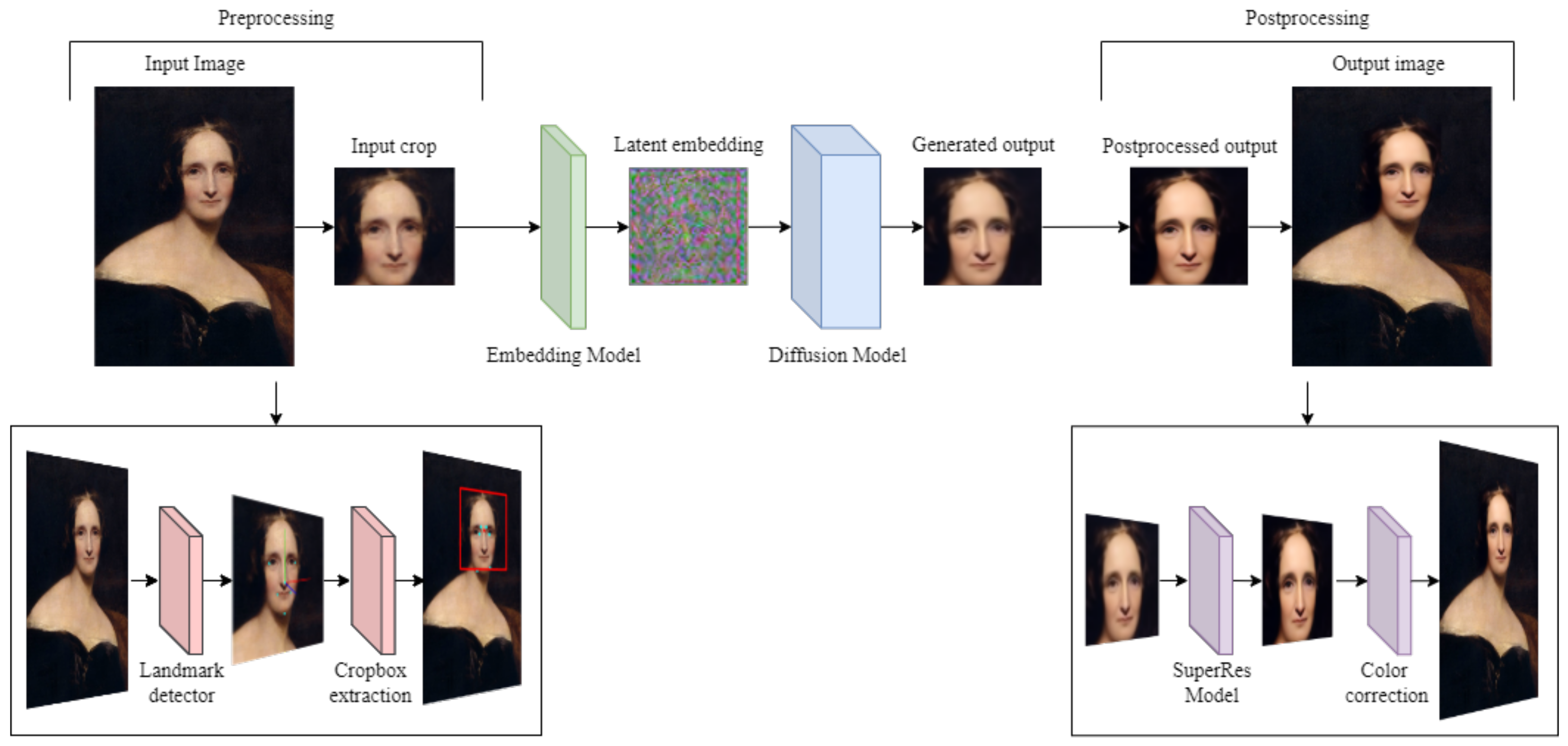
The overall pipeline of the application is quite complex, comprising several nontrivial operations both in the pre-processing and post-processing phases. A synthetic description of the main steps is given in Figure 4.

Pre-processing operations comprise automatic face identification, head pose estimation [13], possible rotation along the roll axis, and cropping. To ensure the effectiveness of the diffusion network, it is essential to maintain consistency with the cropping technique used to create training data. In order to achieve this, it is necessary to detect the relevant facial keypoints that define the boundaries of the face, which will enable accurate and consistent cropping.

During post-processing, we apply a hyper resolution algorithm to obtain a high quality output, recalibrate the colors of the resulting image to better match those of the original portrait, compute and use a background mask together with a progressive alpha-smoothing around the borders to facilitate the re-insertion in the original painting.

The implementation of the pipeline briefly described above requires the deployment of many different technologies discussed in this work. Moreover, the networks for reverse diffusion and embedding have been re-trained and fine-tuned. Additional networks for background segmentation and image super-resolution have been created and trained to further increase the quality of the resulting images.

The article is structured in the following way. In Section 2, we give a pragmatic introduction to denoising models, discussing in particular the pseudocode for training and sampling. A formal introduction to the theory behind denoising diffusion models is outside the scope of this article, and we refer the reader to the extensive literature on the probabilistic foundation of this technique [14,15,16]. In Section 3, we discuss the embedding problem, that is, the computation of a latent encoding $z_x$ for a given input image x; when $z_x$ is passed as input to the reverse diffusion process, this should return the original image x. Preprocessing operations are addressed in Section 4, comprising Face Detection (Section 4.1), Head Pose Estimation (Section 4.2), and cropping (Section 4.3). Postprocessing operations are dealt with in Section 5, covering in particular super resolution (Section 5.1), Face Segmentation (Section 5.2), and Color Correction (Section 5.3). Concluding remarks and ideas for future developments are given in Section 6.

2. Denoising Diffusion Models

Denoising Diffusion Models (DDM) [14] are the new state-of-the-art technology in the field of deep generative modeling, challenging the role previously held by Generative Adversarial Networks [6]. The distinctive properties of this generative technique, shared by many recent applications like [17,18,19], comprise excellent generation quality, high sensibility and responsiveness to conditioning, good sampling diversity, stability of training, and satisfactory scalability.

Roughly, a diffusion model trains a single network to denoise images with a parametric amount of noise; this network is then used to generate new samples by iteratively denoising a given “noisy” image, starting from pure random noise and progressively removing a decreasing amount of noise. Figure 5 provides a straightforward graphical representation.

This process is traditionally called reverse diffusion since it is meant to “invert” the direct diffusion process consisting in iteratively adding noise. In the case of Implicit Diffusion models [15] that we used for our application, reverse diffusion is deterministic.

The only trainable component of the reverse diffusion process is a denoising network ${ϵ}_{\theta }(x_t,{\alpha }_t)$, which takes as input a noisy image $x_t$ and a noise variance ${\alpha }_t$, and tries to guess the noise present in the image. This model is trained as a traditional denoising network, taking a sample $x_0$ from the dataset, corrupting it with a given amount of random noise, and trying to identify the noise in the noisy image.

The pseudocode for training is given in Algorithm 1. We recall that the meaning of the tilde operation $x\sim P$ is to sample x according to the probability distribution P. $P_{\mathit{DATA}}$ is the distribution of data points.

Algorithm 1 Training

1: Fix a noise scheduling $({\alpha }_T,\cdots ,{\alpha }_1)$ 2: repeat 3:     $x_0\sim P_{\mathit{DATA}}$                                                                                                                                                               ▹ take a sample 4:     $t\sim$ Uniform(1,..,T)                                                                                                                                              ▹ choose a timestep 5:     $ϵ\sim \mathcal{N}(0;I)$                                                                                                                                   ▹ create random gaussian noise 6:     $x_t=\sqrt{{\alpha }_t}{x}_0+\sqrt{1-{\alpha }_t}ϵ$                                                                                                ▹ corrupt the sample with noise rate ${\alpha }_t$ 7:     Take gradient descent step on ${\left||ϵ-{ϵ}_{\theta }(x_t,{\alpha }_t)|\right|}^2$                                                                                 ▹ backpropagate the loss 8: until converged

Generative sampling is an iterative process. Starting from a purely noisy image $x_T$, we progressively remove noise by calling the denoising network. The denoised version of the image at timestep t is obtained by inverting step 6 of the training pseudocode, where $x_{t-1}$ plays the role of $x_0$. The pseudocode for sampling is given in Algorithm 2.

Algorithm 2 Sampling

1: $x_T\sim \mathcal{N}(0,I)$ 2: for $t=T,...,1$do 3:     $ϵ={ϵ}_{\theta }(x_t,{\alpha }_t)$                                                                                                                                        ▹ predict noise 4:     ${\tilde{x}}_0=\frac{1}{\sqrt{{\alpha }_t}}(x_t-\frac{1-{\alpha }_t}{\sqrt{1-{\alpha }_t}}ϵ)$                                                                                              ▹ compute denoised result 5:     $x_{t-1}=\sqrt{{\alpha }_{t-1}}{\tilde{x}}_0+\sqrt{1-{\alpha }_{t-1}}ϵ$                                                                                ▹ re-inject noise at rate ${\alpha }_{t-1}$ 6: end for

The usual architecture for the denoising network is that of a U-Net [20], structured with a downsample sequence of layers followed by an upsample sequence, with skip connections added between the layers of the same size.

The noise variance ${\alpha }_t$ is taken as an additional input, vectorized and stacked along the channel axis. To improve the sensibility of the network to this value, ${\alpha }_t$ is frequently embedded using an ad hoc sinusoidal transformation, splitting it into a set of frequencies, in a way similar to positional encodings in transformers [21].

An important aspect in implementing diffusion models is the scheduling of the diffusion noise ${\left\{{\alpha }_t\right\}}_{t=1}^T$ during reverse diffusion. In [14], the authors proposed to use linear or quadratic schedules, but this choice exhibits too steep a decrease during the first time steps, causing problems during generation. Alternative scheduling functions with a gentler decrease have been proposed in the literature, such as the cosine or continuous cosine schedule [22,23]. The choice of a gentler scheduler also allows the model to reduce the number of iterations during generation, which is particularly important for training the embedding network. For our purposes, we used a network with 10 diffusion steps, which is a standard number for DDIM [15]. Augmenting the number of steps only produces minor improvements in the quality of images, largely encompassed by super-resolution post-processing.

3. Embedding

The key contribution of [1] was to show that a neural network could be trained to compute the latent representation $z_x$ of some data sample x. The loss function used to train the model is simply the distance between the original image x and the result $\widehat{x}$ of the denoising process originated from $z_x$. Somewhat surprisingly, the machinery of modern environments for neural computation (we used tensorflow) is enough to smoothly backpropagate gradients through the iterative loop of the reverse diffusion process.

It is worth stressing that embedding is not an iterative process; a single forward pass through the embedding network is enough to compute the latent representation.

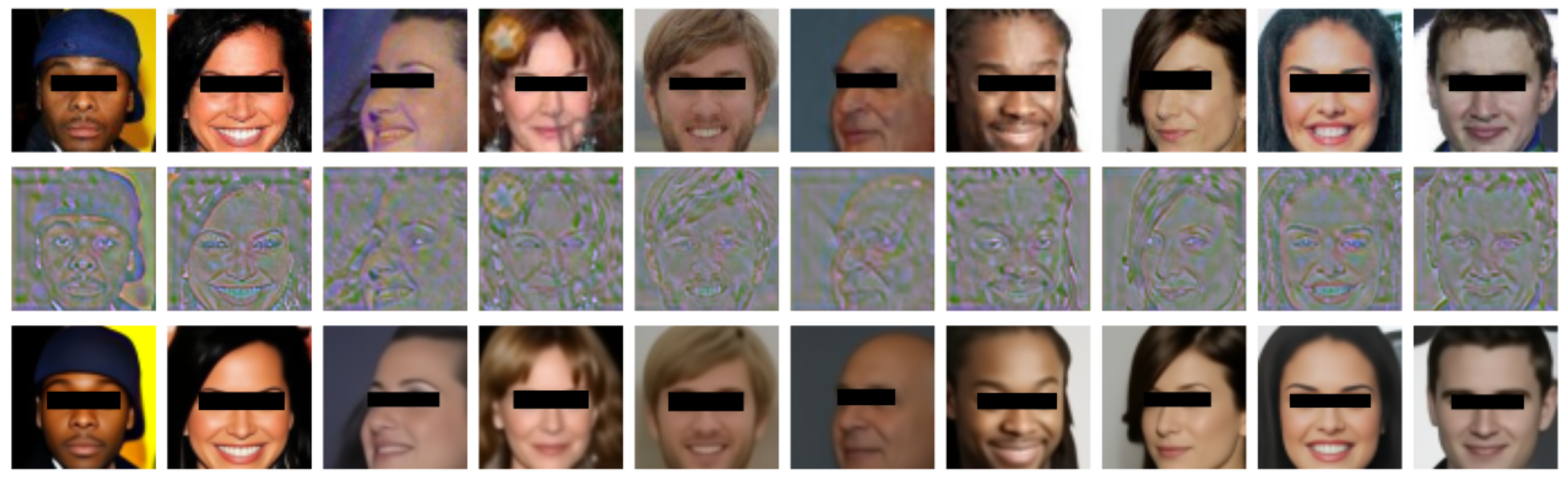
Several different architectures were tested, and a simple U-Net proved to be the best solution. For this article, we trained a new and slightly larger network, marginally improving the already excellent results in [1]. Some examples of embedding and reconstructions are shown in Figure 6; the reconstruction quality is pretty good, with an MSE of around 0.0012 in the case of CelebA [11], with just a slight blurriness. The quality of the embedding can be further increased by a few optional steps of gradient ascent, following the approach described in [1].

We recall that, in the case of diffusion models, the latent space has the same dimensionality of the visible space, so latent encodings can be visually inspected and compared with real images.

Instead of improving the quality of the resulting images by pushing training, which could eventually result in overfitting, we preferred to address the blurriness problem by applying a final super-resolution network, similar to what is done in stable diffusion [24]. The super-resolution network is discussed in Section 5.1.

4. Pre-Processing

The purpose of the pre-processing phase is to automatically extract from the input image the crops of individual faces and to pass them to the embedding generation network. The delicate point is that the crops must respect the size and the alignment of the faces over which the diffusion model has been trained. Since Celeba crops are centered with respect to the position of the eyes, cropping requires the identification of facial landmarks. Below we further describe these operations, along with the software that has been used to address them.

4.1. Face Detection and Landmark Extraction

The first step in the face recognition pipeline is to locate the faces in the input image. To accomplish this, we used the Face Recognition [25] library, a powerful Python library built on top of dlib and deep learning models.

The face detection algorithm used in the Face Recognition library, as stated in the previously cited article, is based on the Histogram of Oriented Gradients (HOG) method. This method involves computing the gradient orientation and magnitude at every pixel in an image, and then grouping these values into cells and blocks. The resulting histogram of these values is then used to identify regions of the image that may contain a face. Once faces have been detected, the Face Recognition library uses a deep learning model to extract facial landmarks. These are key points on the face, such as the corners of the eyes, nose, and mouth, that are important for subsequent analysis. The algorithm uses a convolutional neural network (CNN) trained on a large dataset of faces to accurately locate these landmarks.

As stated by the authors, the model has an accuracy of $99.38\%$ on the Labeled Faces in the Wild benchmark [26].

With its simple APIs for face detection, recognition, and manipulation, the Face Recognition library provides an efficient and accurate way to extract faces from images.

4.2. Head Pose Estimation

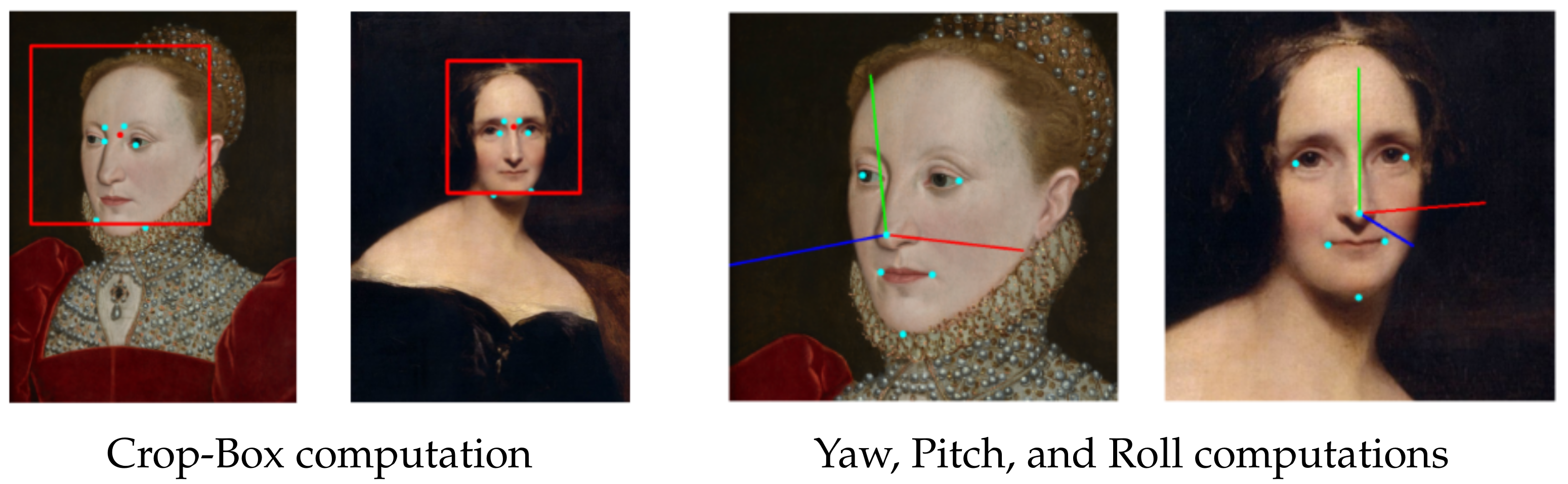
Head pose estimation is a computer vision task that focuses on determining a person’s head orientation in three-dimensional space. This involves calculating three rotation angles, namely yaw, pitch, and roll, which together provide a comprehensive representation of the head’s orientation.

Specifically, yaw refers to the rotation around the vertical axis, pitch corresponds to the rotation around the horizontal axis, and roll represents the rotation around an axis perpendicular to the other two. To compute these angles, we first define a region of interest (ROI) around the face in the input image using the coordinates obtained from the face detection step. Next, we project a selected set of facial landmarks, such as the nose tip, chin, eye corners, and mouth corners, onto the ROI. By combining these projected points with a generic 3D face model, we can estimate the face’s rotation and translation vectors.

To achieve this, we utilize the cv2.solvePnP() function from the OpenCV library [27], which addresses the Perspective-n-Point (PnP) problem. In particular, we employ the iterative method (cv2.SOLVEPNP_ITERATIVE) to refine the estimates. If the estimation is successful, we compute the Euler angles (yaw, pitch, and roll) from the decomposed projection matrix using the cv2.decomposeProjectionMatrix() function, which is based on the following equations:

$$\begin{array}{c}pitch=atan2\left(-R_{2,0},\sqrt{R_{2,1}^2+R_{2,2}^2}\right)\\ yaw=atan2(R_{1,0},R_{0,0})\\ roll=atan2(R_{2,1},R_{2,2})\end{array}$$

(1)

Here, $R_{i,j}$ denotes the entries of the rotation matrix obtained through the cv2.solvePnP() function.

Subsequently, we convert the pitch, yaw, and roll angles from radians to degrees and apply corrections to ensure that these angles lie within the appropriate range, using the following formulas:

$$\begin{array}{c}pitch=arcsin(sin(pitch\left)\right)\\ roll=-arcsin(sin(roll\left)\right)\\ yaw=arcsin(sin(yaw\left)\right)\end{array}$$

(2)

For optimal performance of the diffusion model, we discard faces with yaw angles greater than 50 degrees and faces with pitch and roll angles exceeding 45 degrees. This is because the training was conducted on the CelebA Aligned dataset, which primarily consists of frontal faces. Additionally, we perform a rotation step for faces with roll angles between 15 and 45 degrees to correct their orientation and align them better with the training data. Once the diffusion process is completed, we rotate the faces back to their original orientation, allowing them to be accurately integrated into the original image.

4.3. Cropping

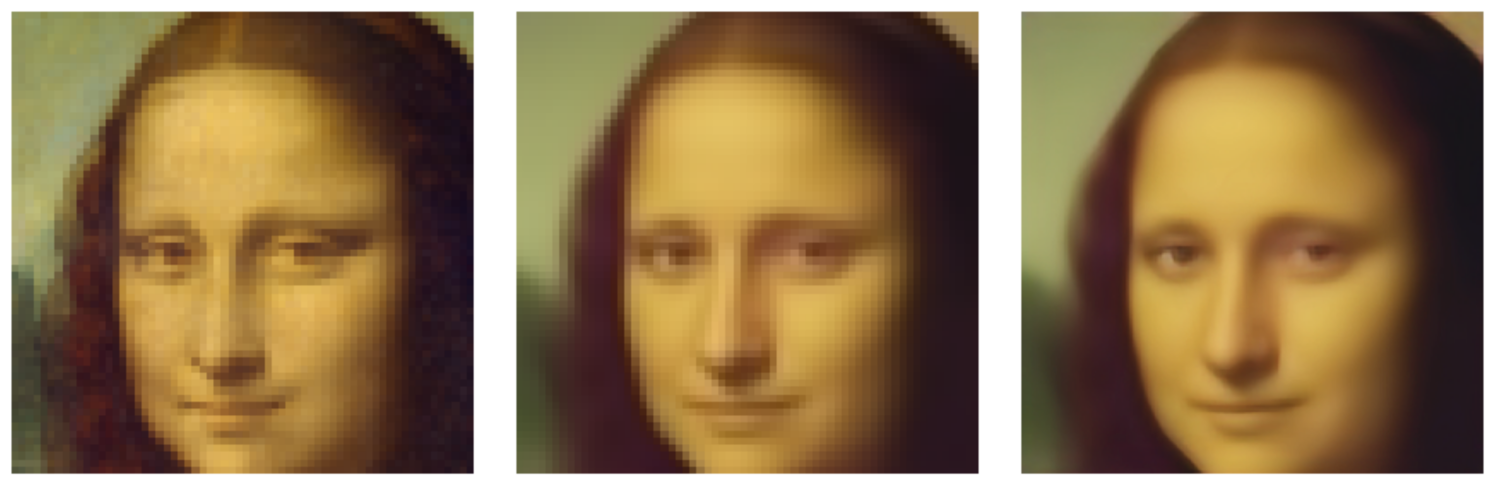
Images used to train the diffusion model are based on a central crop of dimension $128\times 128$ of the CelebA-aligned dataset, frequently used in the literature [28,29]. The size of the crop is meant to facilitate down-sizing to dimension $64\times 64$ that is the actual input–output dimension of the reverse diffusion process. The only minor drawback of this crop is that it typically cuts a small portion of the chin (see Figure 6).

In order to optimize the reification process, we need to crop new faces according to a similar method.

The center of the crop box is computed as an average of the landmarks corresponding to the inner corners of the eyes and the eyebrows. The size of the crop box is double the distance of the center from the average point between the outermost landmarks of the chin. The points used in this process are shown in the first two images of Figure 7.

Once all the crop boxes have been calculated, faces are extracted from the input image and fed into the diffusion model.

4.4. Effect of the Crop on the Face Expression

Most of the images in the CelebA dataset are smiling. This typically results in a bias towards smiling faces during the generative process, which can be annoying. Somewhat surprisingly, the expression can be changed by merely acting on the dimension of the crop. Reducing by a small factor (say, $0.98$) the size of the crop, we accentuate the cheerful appearance, while increasing the size of the box (say, by a factor $1.05$), we may induce a more stern, almost frowning expression (see Figure 8).

We do not have a clear explanation for this phenomenon, which was discovered by chance during fine-tuning of the algorithm. We mention it to highlight the sensibility of the generation process to small perturbations of the latent encoding, and to stress the complexity of discovering interesting semantic trajectories in the huge latent space of diffusion models. Similarly, it clarifies the difficulty of fully automatizing the cropping phase, which could require some supervised fine-tuning to obtain really satisfactory results.

5. Post-Processing

To enhance the integration of the diffusion model’s results with the original image, a post-processing pipeline that employs various techniques is employed.

Our post-processing pipeline includes a super-resolution model and a segmentation model, both of which are essential for enhancing the quality of the reconstructed images. Instead of using existing pre-trained models in the literature, such as ESRGAN for super-resolution [30], we decided to implement and train these models from scratch.

By developing our models from scratch, we were able to create models that are specifically tailored to the task of processing faces, resulting in lighter and faster models that are optimized for our specific needs.

Furthermore, by not using a model trained with adversarial training, such as a GAN model, we can be certain that the output does not contain artifacts not present in the original image.

In this section, a detailed description of the above-mentioned techniques is provided.

5.1. Super-Resolution

In the initial stage, a super-resolution model is employed to enhance the resolution of the diffusion model’s output images. The images generated by the diffusion model have a size of 64 × 64 pixels, and to improve their visual quality, a specially trained face super-resolution model is utilized. The purpose of this model is to increase the size of the images by a factor of four, resulting in an output image size of 256 × 256 pixels. This process is essential to enhance the image resolution and produce high-quality output images.

Our proposed super-resolution architecture is inspired by the generator architecture proposed in [31], which has been widely used in the field of image processing. We extended this architecture by incorporating the Self-Attention Mechanism, as suggested in [32].

The overall architecture is described in Figure 9.

It exploits self-attention layers and residual blocks. The self-attention mechanism is meant to capture long-range dependencies in the image, and the residual blocks help to avoid the vanishing gradient problem and accelerate the training process. In detail, it consists of a skip connection followed by 16 residual blocks, each of which is followed by a self-attention module. The output of the residual blocks is then concatenated with the skip connection, and the resulting tensor is upsampled using two upsampling blocks.

To ensure consistency with the training dataset of the diffusion model, the super-resolution model was trained on a cropped version of CelebAMask-HQ [33]. CelebAMask-HQ is composed of 30,000 images of the primary CelebA dataset, but at higher resolution. Furthermore, these images come with segmentation masks of facial features and accessories, including skin, eyes, nose, ears, hair, neck, mouth, lips, hats, eyeglasses, jewelry, and clothes, which have not been used for the super-resolution task.

To train the super-resolution network, we used a custom loss combining mean squared error (MSE) and perceptual loss, with equal weights assigned to each component. The perceptual loss is computed based on the VGG-19 [34] neural network. By using this custom loss function, the model is able to optimize both the quantitative metrics captured by MSE, as well as the perceptual quality of the output images.

5.2. Faces Segmentation

A potential issue hindering the quality of reconstructed images is related to background elements, traditionally difficult to render for generative techniques, due to their large variability. To address this problem, we introduced a segmentation phase to effectively identify and remove the background.

We performed the segmentation on a region of interest (ROI) that contains the face in the original image. The resulting mask is then cropped to match the Diffusion Model-generated face and used to remove the background from the reconstructed image. To implement the segmentation process, we trained a U-Net model [20] on the CelebaMask-HQ dataset, which includes high-quality face masks manually annotated. This allowed us to precisely segment the face region with an accuracy of $96.78\%$ and a recall of $97.60\%$.

To further enhance the appearance of the reconstructed image, we employ a fading technique to gradually blend the border of the generated face with the original image. This technique helps to avoid sharp edges or visible borders that could negatively impact the final result, ensuring a more natural and seamless appearance (see Figure 10).

An example of segmentation masks can be found in Figure 11. Overall, the segmentation process and the fading technique have significantly improved the quality of our reconstructed images, allowing us to produce more accurate and visually appealing results.

5.3. Color Correction

As a final step, we applied a color correction technique to mitigate color discrepancies between generated faces and their respective sources, improving the overall visual coherence and realism of the results.

The color correction operation aligns the color statistics of two images using the Lab color space. It involves several steps, including converting the images to Lab color space, normalizing the Lab channels of the target image using the mean and standard deviation of the source image, and converting the target image back to RGB color space. All the steps are explained in Algorithm 3.

Algorithm 3 Color correction

1: lab_target = convert_color_space(target_image, "RGB", "LAB") 2: lab_source = convert_color_space(source_image, "RGB", "LAB") 3: mean_target = compute_mean(lab_target) 4: mean_source = compute_mean(lab_source) 5: std_target = compute_standard_deviation(lab_target) 6: std_source = compute_standard_deviation(lab_source) 7: lab_target = $\left(\frac{(\mathrm{lab\_target} -\mathrm{mean\_target} )}{\mathrm{std\_target} }\right)$× std_source + mean_source 8: target_image = convert_color_space(lab_target, "LAB", "RGB")

The LAB color space is often used in color correction algorithms because it separates the luminance (brightness) component from the chrominance (color) information. This makes it easier to manipulate the color information separately from the brightness information, making the color correction more reliable. In Figure 12 we give an example demonstrating the effect of the entire post-processing phase.

6. Conclusions

In this article we presented a complete application for the transformation of a painter’s portrait into a real human face; we call this process portrait reification. The heart of the application is the embedding procedure for generative diffusion models recently introduced in [1]. Since the diffusion model was trained to generate human faces, it will revert the embedding of the portrait into the most likely real approximation of the original subject.

In order to turn this simple idea into a stand-alone and fully functional application, several steps have been required, both during pre-processing and post-processing.

Pre-processing operations comprise automatic face identification, head pose estimation, possible rotation along the roll axis, and cropping. Cropping is particularly delicate, since it must be coherent with the face crops used to train the generative model; a correct computation of the crop eventually requires the identification of the main facial keypoints. In addition, we also discovered that small modifications of the crop dimension may sensibly change the expression of the generated face.

In the postprocessing phase, we apply a hyper resolution algorithm to obtain a high-quality output, recalibrate the colors of the resulting image to better match those of the original portrait, compute a background mask to preserve the original background, and finally use progressive alpha-smoothing around the borders to facilitate merging into the original painting.

The application works well for most naturalistic styles, but it could be in trouble on some modern styles such as Cubism, Surrealism, Pointillism, and Expressionism, not always presenting clear and recognizable facial features. In case the face is correctly identified, some manual editing of the latent encoding and fine-tuning of the different phases could be required.

Beyond the amusing functionality provided by the application, the interest of the work consists in attesting the complexity of interacting with the latent representation of diffusion models, mostly due to their high dimensionality, equal to the dimension of the real space. Tiny modifications of the latent encoding easily result in sensible modifications of the generated image, comprising expression, gender, and even orientation. The impact of the face crop on the expression of the face seems to suggest that, in the case of diffusion models, vector adjustments along suitable trajectories might not be enough to obtain interesting editing effects, but more complex topological operations, e.g., dilation or contraction, could be required.