Modeling of Physical Activity Behavioral Interventions Relying on MPC Strategy

Abstract

Physical inactivity is becoming an important threat to public health in today’s society. The COVID-19 pandemic has also reduced physical activity (PA) levels given all the restrictions imposed worldwide. In this work, physical activity interventions supported by mobile devices and relying on control engineering principles were proposed. The model was constructed relying on previous studies that consider a fluid analogy of Social Cognitive Theory (SCT), which is a psychological theory that describes how people acquire and maintain certain behaviors, including health-promoting behaviors, through the interplay of personal, environmental, and behavioral factors. The obtained model was validated using secondary data (collected earlier) from a real intervention with a group of male subjects in Great Britain. The present model was extended with new technology for a better understanding of behavior change interventions. This involved the use of applications, such as phone-based ecological momentary assessments, to collect behavioral data and the inclusion of simulations with logical reward conditions for reaching the behavioral threshold. A goal of 10,000 steps per day is recommended due to the significant link observed between higher daily step counts and lower mortality risk. The intervention was designed using a Model Predictive Control (MPC) algorithm configured to obtain a desired performance. The system was tested and validated using simulation scenarios that resemble different situations that may occur in a real setting.

1. Introduction

According to the World Health Organization (WHO), physical inactivity is becoming a serious problem worldwide. Sedentary people tend to develop major health issues, most needing long-term treatments or continuous medication. In some countries, people without private insurance rely on local government health providers to be treated. Consequently, governments are held responsible for the health, treatment, and medical care of millions of citizens which causes a huge economic impact. On the other hand, physical activity (PA) decreases emotional stress and improves physical and psychological health [1]. The COVID-19 pandemic has had unprecedented health, economic, and social consequences worldwide causing a decrease in physical activity and a deterioration in physical and psychological health [2,3,4].

Different organizations (i.e., National Institutes of Health (NIH) or American Council on Exercise (ACE)) are trying to encourage people to engage more in physical activity and are involved in research on how to do this effectively [5,6]. As part of the aforementioned research, Behavioral Intervention models were developed based on Bandura’s Social Cognitive Theory (SCT) [7,8,9]. Fortunately, to mitigate the problem of sedentary behavior, recent technologies have opened new ways for intervening upon behavior via mobile applications to improve and test models with data that can be collected easily, using “patient-friendly” ideas [10].

For some years now, control system engineering principles have been proposed to address problems in behavioral medicine [11,12]. In this work, a control strategy was proposed that relies on an SCT model obtained from secondary data (information that was collected and analyzed by someone else for a different purpose but can be reused for a new research project) and tested on a different model obtained from primary data (information that is original and has not been collected or analyzed by anyone else for a different purpose) to address the physical inactivity issue.

In summary, this paper presents a model approach to simulating and managing dynamic multivariable systems using Model Predictive Control (MPC), which has gained significant traction in the biomedical engineering and control systems field. It involves creating a model of the system being controlled and using that model to predict future behavior and optimize control inputs accordingly [13,14].

The paper is organized as follows. Section 2 presents a modeling procedure obtained from previous research regarding Behavioral Intervention problems and the challenges that arose. Section 3 describes the proposed control strategy for Behavioral Intervention. Section 4 provides the details of the results of the analysis obtained from a simulation using the proposed controller. Section 5 gives a summary of conclusions and future work.

2. Modeling Procedure

Bandura’s Social Cognitive Theory (SCT) is a widely used framework for behavior change strategies, providing a basis for understanding behavior and its relationships. 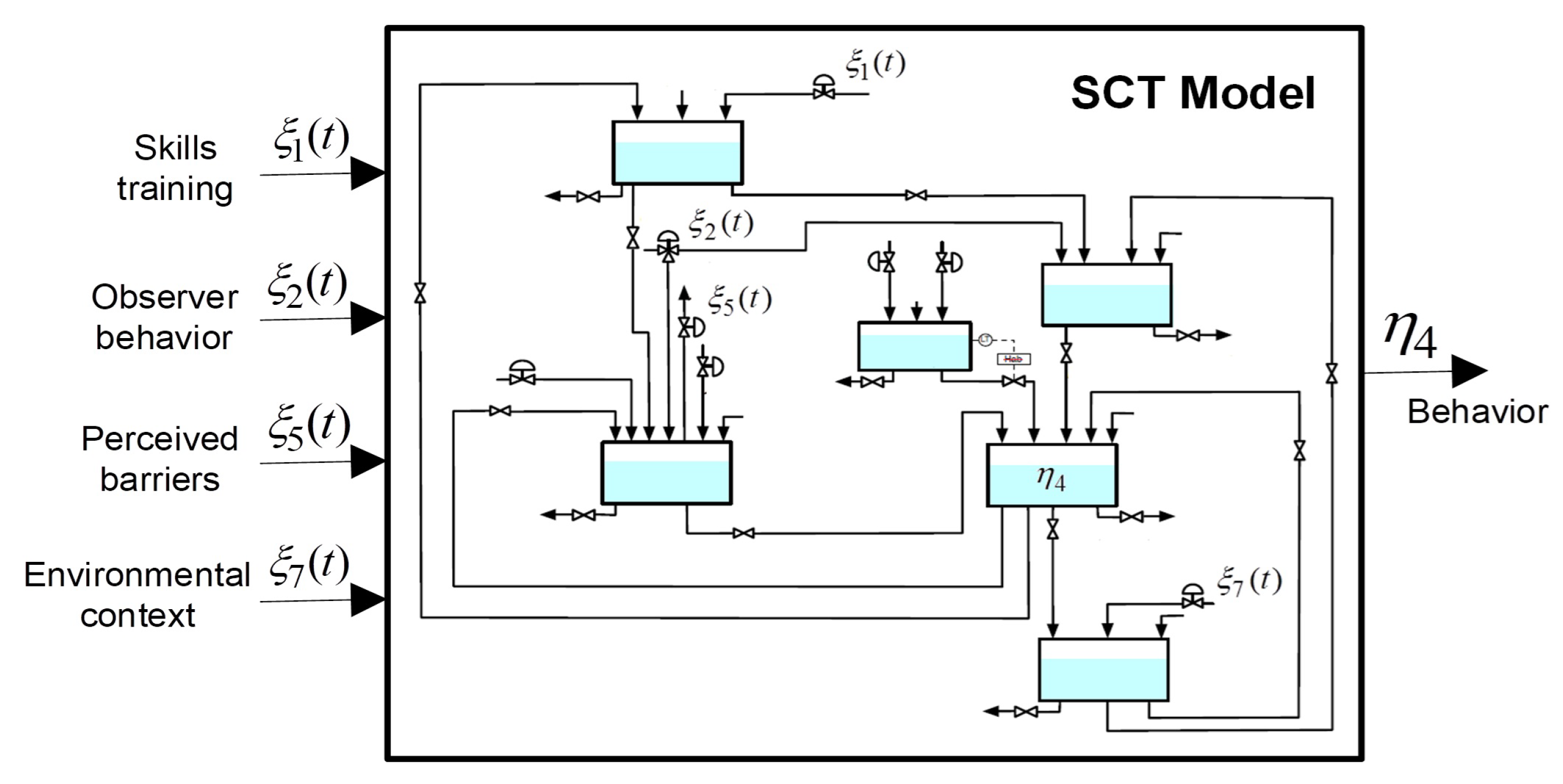SCT emphasizes reciprocal determinism, where personal factors, environmental factors, and behavior interact and mutually affect each other; in other words, that both personal and environmental factors contribute to shaping behavior and, in turn, behavior also influences personal and environmental factors [7]. Using a fluid analogy can help to create a structured framework and mathematical model of behavioral performance in a simple way, representing Bandura’s SCT constructs and their interrelationships. The outputs are treated as levels of tanks (constructs), while the other signals are treated as inputs to those inventories. Behavior is represented as a fluid inventory that changes over time $\left(t\right)$ based on various SCT factors. The model was developed on a daily time frame and could be adapted for different behaviors and time frames of interest [15]. The levels of tanks are represented by the variables ${\eta }_i$ and exogenous inputs are represented in the diagram by variables ${\xi }_i$. The inflow resistances are denoted by ${\gamma }_i$ and outflow resistances are represented by ${\beta }_i$. These resistances can be interpreted as the fraction of each inventory or input that flows from one instance to the next. Other parameters represent the physical characteristics of each inventory and flow, including time constants ${\tau }_i$ and time delays ${\theta }_i$. Unmeasured disturbances are considered as ${\zeta }_i$.

By means of a fluid analogy of SCT, computational approaches can be used to model and test these relationships, while mobile and wireless technologies can help measure them in real-time. SCT has proven successful in mobile health interventions for biomedical engineering and applications such as smoking cessation, weight management, and management of physical inactivity [8].

A procedure for identifying a dynamic model of a Social Norm Physical Activity Intervention was proposed using a semi-physical system and data from a randomized controlled trial [9,16]. However, the secondary data model needs to be improved in order to meet the necessary conditions for the proposed behavior change intervention.

2.1. Secondary Data Modeling

A model was created through secondary data analysis of a randomized controlled trial conducted in the United Kingdom, which suggested that smartphones are effective at motivating individuals with limited intrinsic motivation for exercise to engage in physical activity [16]. There were three groups of 55 male adult participants each. Data from participant number 115 were used for the semi-physical identification because he had the most reliable set of data for the study period with the least amount of missing information.

The structure of the intervention is based on a simplified version of the dynamical systems model of the Social Cognitive Theory (SCT) presented by Martín et al. [15], which is illustrated as a fluid analogy in Figure 1. The only output considered is the behavior (${\eta }_4$), which is measured through the number of daily steps taken by the individual. This “subsystem” is used to describe the algorithm of physical activity intervention related to social norms to encourage physical activity behavior.

The simplified model included inputs (${\xi }_1$), (${\xi }_2$), (${\xi }_5$) and (${\xi }_7$), while ignoring inputs (${\xi }_3$) (Persuasion), (${\xi }_4$) (Internal Cues), and (${\xi }_6$) (Intrapersonal States) as they were irrelevant to the study. These inputs will be assumed to be equal to zero. The meaning of some inputs is:

• Skills training (${\xi }_1$). These activities help to increase (or decrease) the self-management skills of the individual.
• Observed behavior of others (${\xi }_2$). This input refers to vicarious learning or social learning. This is a type of learning that occurs when an individual can acquire knowledge and skills by observing others and learning from the outcomes of their actions.
• Perceived barriers (${\xi }_5$). This input refers to external conditions that affect behavior. For instance, unfavorable weather conditions, limited availability of exercise facilities, or insufficiently secure walking paths can all hinder physical activity levels. This input refers to conditions that are perceived by the participants.
• Environmental context (${\xi }_7$). This input refers to situational factors which directly influence the behavioral outcomes. This study takes into account the date of measurement, which is identified as either a weekend or a weekday.

This approach used principles from semi-physical system identification and relied on the widely-accepted prediction–error identification methods (PEM) [17]. Semi-physical identification combines physical knowledge and experimental data to create a mathematical model of a physical system (which was created based on the data obtained from male subjects in Great Britain and was previously presented in an earlier study published in 2016) [16]. It involves using simplified physical models or analogies to represent a complex system (human behavior can be considered a complex system, composed of interconnected components that interact nonlinearly) and then fitting experimental data to these models to estimate system parameters. This approach can be used to predict the system’s behavior under different conditions.

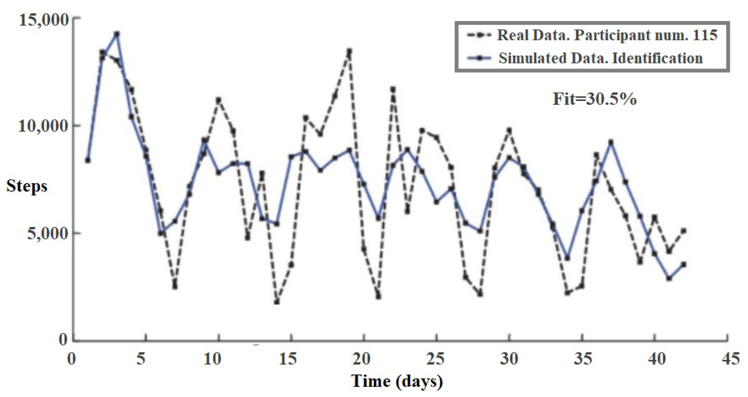
The estimation process was carried out in MATLAB^® using the idgrey and greyest commands from the System Identification Toolbox [18]. The idgrey model is used to represent a system as a state-space model with identifiable coefficients. The greyest function is employed to estimate the unknown parameters of the idgrey model. Results obtained are depicted in Figure 2. By comparing the estimated behavior (${\eta }_4$) based on the number of steps obtained from semi-physical identification using simulated data with the real experimental data from male adult participant number 115, a fitting of 30.5% was achieved with nine iterations, which serves as a good starting point.

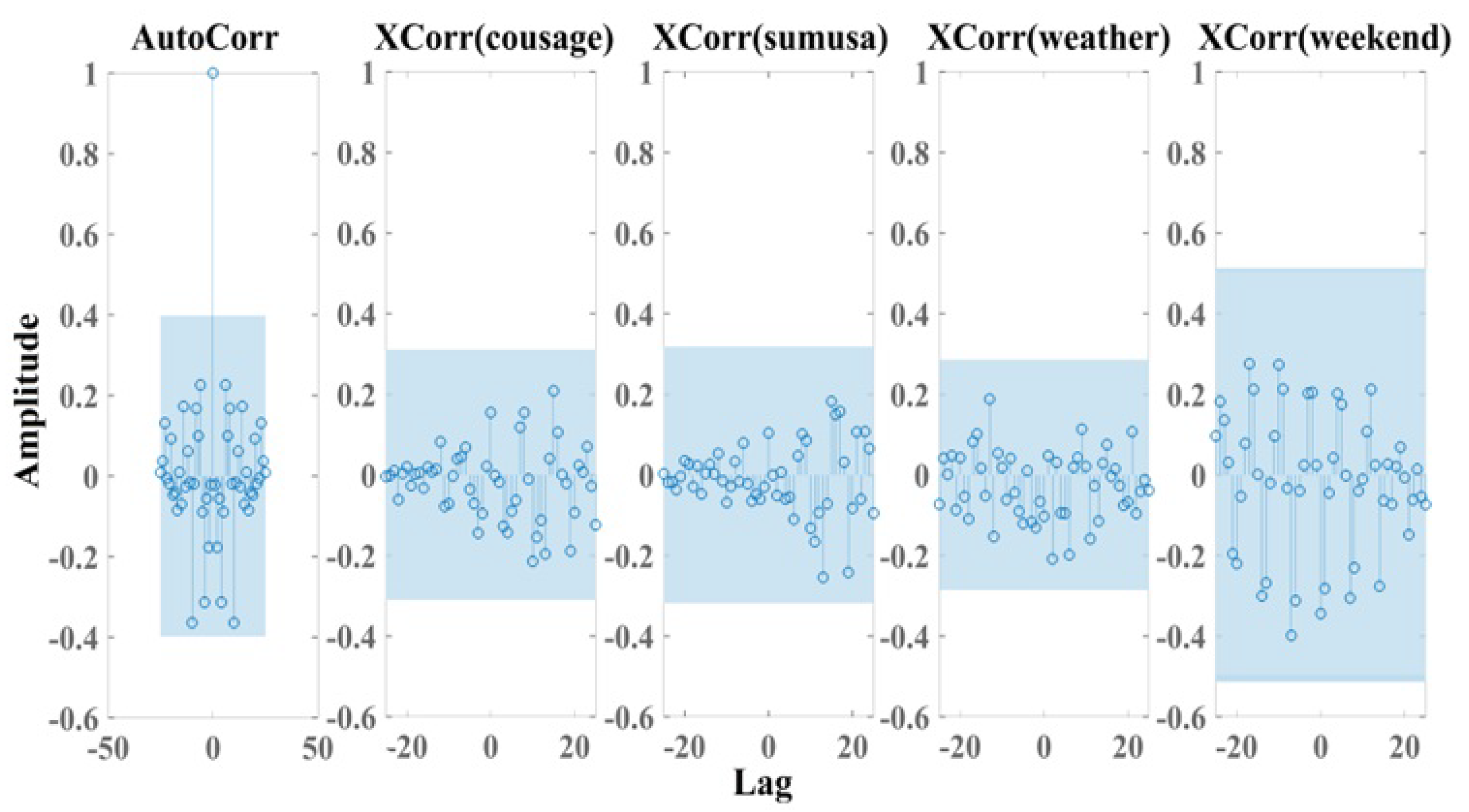
Additionally, a validation procedure relying on correlation analysis was performed for a semi-physical identification method resulting in residual errors within confidence bounds. The autocorrelation for behavior and cross-correlation for different lags between behavior and each of the following variables are shown in Figure 3, where:

• “Co-usage”⇔“skills training” corresponds to the daily number of glances at the application.
• “Sumusa” is “sum of application usage”⇔“observed behavior” is the total length of time (in seconds) per day the application was glanced at.
• “Weather”⇔“perceived barriers” means the environmental condition in which the subject is influenced to engage in physical activity or not.
• “Weekend”⇔“environmental context” indicates whether the date of measurement falls or does not fall during the weekend.

Lag refers to a time delay or temporal shift between two variables. Therefore, when calculating correlation with lag, the relationship between the two variables was analyzed with a certain time delay to see if there was any significant correlation between them at that specific moment.

Correlation analysis is a statistical method that measures the strength and direction of the relationship between two variables. It uses the correlation coefficient, with the amplitude ranging from −1 to 1, where −1 indicates a perfect negative correlation, 0 indicates no correlation, and 1 indicates a perfect positive correlation. To confirm the predictive ability of the model [9], it was expected that the amplitude of autocorrelation would be equal to 1 at zero lag and would take any value within the confidence interval for other lags, if the model is reliable. Moreover, the values within the confidence bounds depicted in Figure 3 in the cross-correlation plots validate the reliability of the model [19].

Although the percentage fit was relatively low, the model developed in [9] is able to follow some of the dynamic characteristics of the system (i.e., amplitude and frequency variations of the signal ${\eta }_4$ over time), even though it was derived from secondary data. Nevertheless, the model has limited applicability for the required purpose since it does not support the implementation of behavioral interventions using external cues or reinforcement through outcome expectancy.

As a result of the previous analysis, internal parameters for the secondary data SCT model were obtained [9]. For the intervention design, this SCT model needs to be expanded to include additional input variables directly associated with the required behavior change intervention. Thus, the secondary data model was expanded with parameters obtained from different experiments where preliminary validated models were obtained using primary data [11,20].

2.2. Hypothetical Model

A second extended model is now considered including additional parameters and intervention inputs. For this purpose, an SCT model enhanced with individualized self-regulation via internalized cues is shown in Figure 4. In the case of this model, too, the daily number of steps was used as a measure of behavior (${\eta }_4$). The primary aim of the intervention proposal is to promote physical activity among inactive individuals, with the specific target of achieving an average of 10,000 daily steps per week in light of the observed significant negative correlation between daily step counts and mortality risk [21]. To motivate participants, the intervention’s conceptual diagram incorporates a reward system. The model includes the following inputs and outputs:

• Environmental context (${\xi }_7$), social and physical factors that affect behavior.
• External cues (${\xi }_8$), triggers to engage in the behavior.
• Expected points (${\xi }_9$), the expected daily reward points that will be exchanged for specific rewards.
• Granted points (${\xi }_{10}$), which are fed to the behavioral outcomes (${\eta }_5$) inventory only if the performed behavior (${\eta }_4$) meets or exceeds the specified goal ($u_8$).
• Goal attainment (${\xi }_{11}$), a new input signal that indicates the amount of attainment of the established goals.
• Outcome expectancy (${\eta }_2$), the perceived probability that performing a given behavior will result in specific outcomes.
• Self-efficacy (${\eta }_3$), the self-perceived capability to perform the required behavior.
• Behavior (${\eta }_4$), the behavior of interest, e.g., daily performed steps.
• Behavioral outcomes (${\eta }_5$), positive or negative outcomes resulting from the behavior, e.g., lost weight, physical pain.

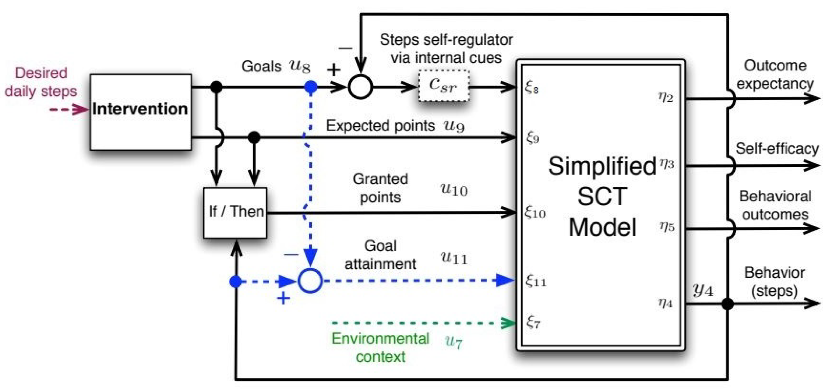
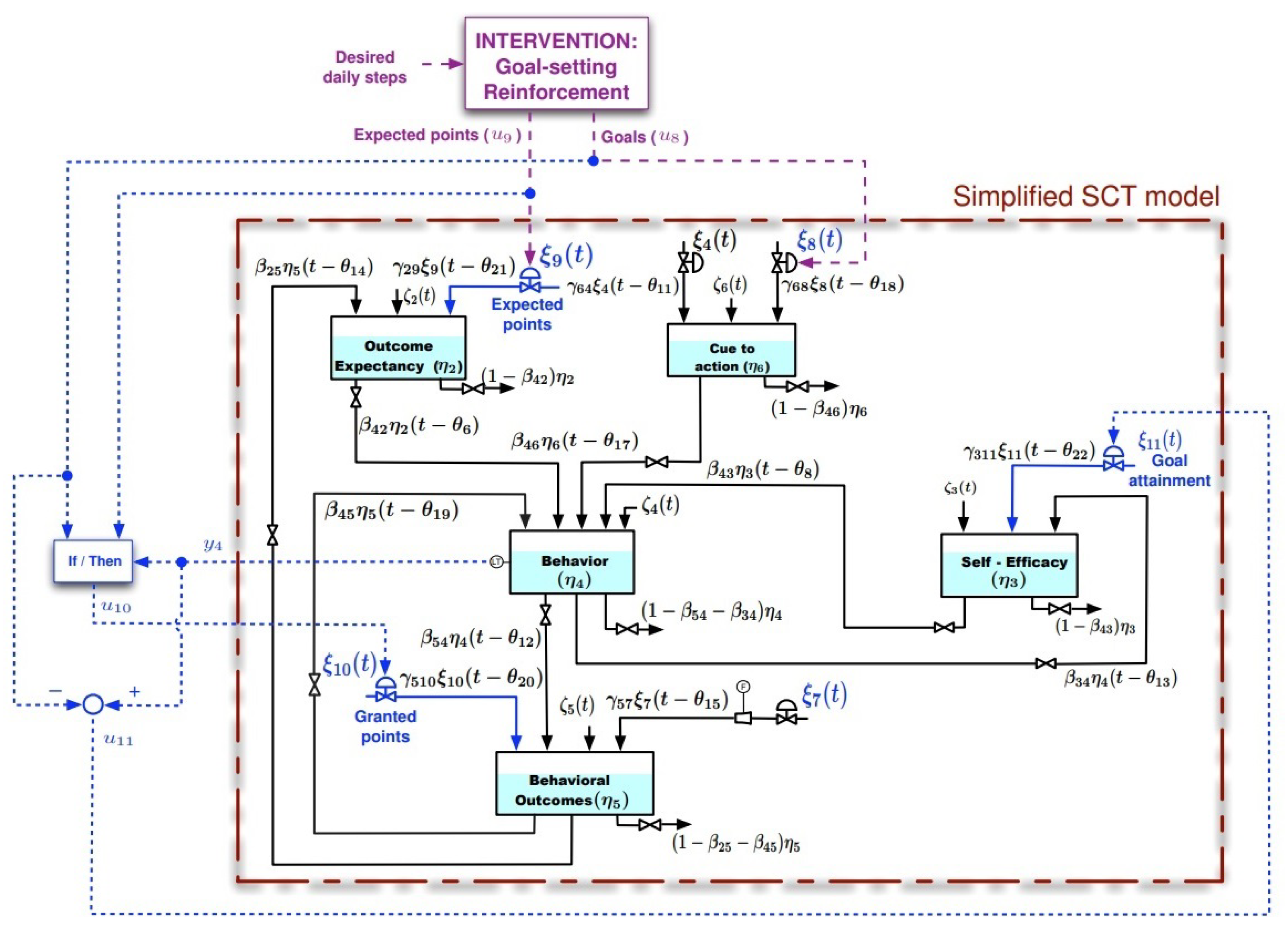
The simplified SCT model upon which the physical activity intervention design with goal setting is based is illustrated in Figure 5, where:

• Daily goals $\left(u_8\right)$, to quantitatively establish the desired behavior, e.g., 10,000 steps per day.
• Expected points $\left(u_9\right)$, the daily reward points announced that will be given to individuals if they achieve the daily goal.
• Granted points $\left(u_{10}\right)$, given every day if individuals meet the established goal; this feature is represented by the “if/then” block. The points can be redeemed later for tangible rewards, such as gift cards.
• Goal attainment $\left(u_{11}\right)$ = ${\xi }_{11}$ = $y_4-u_8$, a signal that represents the gap between the actual behavior and daily goals. It can be used as an input for the self-efficacy inventory and as an output to evaluate the effectiveness of the intervention.

The fluid analogy allows the use of the conservation of mass principle to calculate the accumulation of each inventory based on the net difference between mass inflows and outflows over time domain t. It relates to how a system or signal changes over time. Variables ${\xi }_i$ represent external excitations (i.e., inputs), ${\eta }_i$ are the inventory levels (i.e., outputs), ${\gamma }_1$ and ${\beta }_1$ are factors that represent interactions among the different constructs, ${\zeta }_i$ are external disturbances, and ${\theta }_i$ are delay times. The fluid analogy can be represented by the following system of first-order differential equations: Equations (1)–(5).

$${\tau }_2\frac{d{\eta }_2}{dt}={\gamma }_{29}{\xi }_9(t-{\theta }_{21})+{\beta }_{25}{\eta }_5(t-{\theta }_{14})-{\eta }_2\left(t\right)+{\zeta }_2\left(t\right)$$

(1)

$${\tau }_3\frac{d{\eta }_3}{dt}={\gamma }_{311}{\xi }_{11}(t-{\theta }_{22})+{\beta }_{34}{\eta }_4(t-{\theta }_{13})-{\eta }_3\left(t\right)+{\zeta }_3\left(t\right)$$

(2)

$${\tau }_4\frac{d{\eta }_4}{dt}={\beta }_{42}{\eta }_2(t-{\theta }_6)+{\beta }_{43}{\eta }_3(t-{\theta }_8)+{\beta }_{46}{\eta }_6(t-{\theta }_{17})+{\beta }_{45}{\eta }_5(t-{\theta }_{19})-{\eta }_4\left(t\right)+{\zeta }_4\left(t\right)$$

(3)

$${\tau }_5\frac{d{\eta }_5}{dt}={\gamma }_{57}{\xi }_7(t-{\theta }_{15})+{\gamma }_{510}{\xi }_{10}(t-{\theta }_{20})+{\beta }_{54}{\eta }_4(t-{\theta }_{12})-{\eta }_5\left(t\right)+{\zeta }_5\left(t\right)$$

(4)

$${\tau }_6\frac{d{\eta }_6}{dt}={\gamma }_{64}{\xi }_4(t-{\theta }_{11})+{\gamma }_{68}{\xi }_8(t-{\theta }_{18})-{\eta }_6\left(t\right)+{\zeta }_6\left(t\right).$$

(5)

The extended model includes two additional components. The first one is incorporating an optimal range for step goals. This was accomplished by adding a goal attainment signal that affects self-efficacy based on the effectiveness of the required behavior. Secondly, a self-regulation loop was established by using internal cues and is represented by the $C_{sr}$ block. The idea behind this block is derived from internal model control (IMC) [23]) and is mathematically defined in the equation outlined in [11]. The self-regulation process is represented through a controller that adjusts action cues based on the discrepancies between the set goal ($u_8$) and the measured outcome ($y_4$). The controller needs to allow for a partial set point tracking to permit other intervention components (such as points) to influence changes in the output. According to the IMC formulation, the self-regulator is a classical feedback controller. See Equation (6).

$$c_{sr}=\frac{K_{sr}}{{\gamma }_{64}{\beta }_{46}}\frac{{\tau }_{4}s+1}{\lambda s-K_{sr}+1}.$$

(6)

The performance of the self-regulator is determined by two parameters: $\lambda$, which indicates the closed-loop speed of response, and $K_{sr}$, which ranges between 0 and 1 and represents the level of integral action, with 1 indicating perfect integral action. Equations (1)–(5), without disturbances or delays (${\zeta }_i=0$, ${\theta }_i=0$, ${\forall }_i$), and self-regulator $C_{sr}$, with state ${\eta }_7$, were considered. Assuming that the dominant effect on the output is obtained from the time constant of the behavior inventory (${\eta }_4$), the state matrices are shown in Equations (Section 2.2)–(9).

$$A=\left[\begin{array}{cccccc}\frac{-1}{{\tau }_2}& 0& 0& \frac{{\beta }_{25}}{{\tau }_2}& 0& 0\\ 0& \frac{-1}{{\tau }_3}& \frac{{\beta }_{34}+{\gamma }_{311}}{{\tau }_3}& 0& 0& 0\\ \frac{{\beta }_{42}}{{\tau }_4}& \frac{{\beta }_{43}}{{\tau }_4}& \frac{-1}{{\tau }_4}& \frac{{\beta }_{45}}{{\tau }_4}& \frac{{\beta }_{46}}{{\tau }_4}& 0\\ 0& 0& \frac{{\beta }_{54}}{{\tau }_5}& \frac{-1}{{\tau }_5}& 0& 0\\ 0& 0& \frac{-{\gamma }_{64}{M}_{sr}{\tau }_4}{{\tau }_6}& 0& \frac{-1}{{\tau }_6}& \frac{-{\gamma }_{64}{M}_{sr}(1-N_{sr}{\tau }_4){\tau }_4}{{\tau }_6}\\ 0& 0& -1& 0& 0& -N_{sr}\end{array}\right]$$

(7)

$$B=\left[\begin{array}{ccccc}0& 0& \frac{{\gamma }_{29}}{{\tau }_2}& 0& 0\\ 0& \frac{-{\gamma }_{311}}{{\tau }_3}& 0& 0& \frac{{\gamma }_{34}}{{\tau }_3}\\ 0& 0& 0& 0& 0\\ \frac{{\gamma }_{57}}{{\tau }_5}& 0& 0& \frac{{\gamma }_{510}}{{\tau }_5}& 0\\ 0& \frac{{\gamma }_{64}{M}_{sr}{\tau }_4}{{\tau }_6}& 0& 0& 0\\ 0& 1& 0& 0& 0\end{array}\right]$$

(8)

$$C=\left[\begin{array}{cccccc}1& 0& 0& 0& 0& 0\\ 0& 1& 0& 0& 0& 0\\ 0& 0& 1& 0& 0& 0\\ 0& 0& 0& 1& 0& 0\end{array}\right]$$

(9)

where:

$$M_{sr}=\frac{K_{sr}}{{\gamma }_{64}{\beta }_{46}\lambda }$$

(10)

$$N_{sr}=\frac{1-K_{sr}}{\lambda }.$$

(11)

A stimulus in the form of a reward mechanism was employed to encourage the desired behavior in the intervention, whereby users receive a specified number of points (${\xi }_9$) upon reaching their daily step goals ($u_8$). These points can later be exchanged for tangible rewards. This is represented by an if/then block that is considered external to the simplified SCT model due to its non-linear nature, as depicted in Figure 4.

The obtained model can be described by means of the parameters shown in

Table 1. Parameters of the hypothetical model (i.e., the secondary data model, which was extended with parameters obtained from different experiments using primary data [11,20].

Parameter	Value	Parameter	Value
${\tau }_1$	0.01	${\gamma }_{68}$	1.5
${\tau }_2$	0.1236	${\gamma }_{311}$	0.4
${\tau }_3$	0.01	${\gamma }_{510}$	0.6
${\tau }_4$	0.8	${\beta }_{14}$	0.01
${\tau }_5$	2	${\beta }_{21}$	0.0513
${\tau }_6$	0.5	${\beta }_{25}$	0.5
${\gamma }_{11}$	4.55	${\beta }_{31}$	0.0198
${\gamma }_{22}$	15	${\beta }_{34}$	0.2
${\gamma }_{29}$	2.5	${\beta }_{42}$	1.8437
${\gamma }_{32}$	10.7036	${\beta }_{43}$	0.9
${\gamma }_{33}$	0.5	${\beta }_{45}$	0.5
${\gamma }_{35}$	1	${\beta }_{46}$	1.8755
${\gamma }_{36}$	1	${\beta }_{54}$	0.6
${\gamma }_{57}$	1	$K_f$	0.8
${\gamma }_{64}$	1	$\lambda$	1

, which were partially obtained through Secondary Data Modeling in Section 2.1, using a semi-physical estimation procedure (combining physical knowledge and experimental data to create a mathematical model).

3. Control Strategy

The control strategy for the intervention must incorporate the defined requirements and constraints for physical activity behavioral intervention. Model Predictive Control (MPC) is a controller formulation whereby the current values of the manipulated variables are determined in real-time as the solution of an optimal control problem over a horizon of a given length [14]. In MPC, “move horizon” refers to the number of future control moves computed by the controller at each time step. These future moves are then used to optimize the control actions over a finite time horizon. The “move horizon” length is a key design parameter in MPC, as it affects the trade-off between computational complexity and control performance. A more extended move horizon allows for better prediction and optimization of future behavior but requires more computation time. The optimization problem is solved for a move horizon using a “hypothetical model”, from where a new set of control moves are obtained [22]. Therefore the success of MPC depends on the degree of precision of the model. Only the first calculated move is applied at each instant; the whole process is repeated and new control moves are obtained.

3.1. Open-Loop Behavioral Interventions Analysis: Tuning of MPC

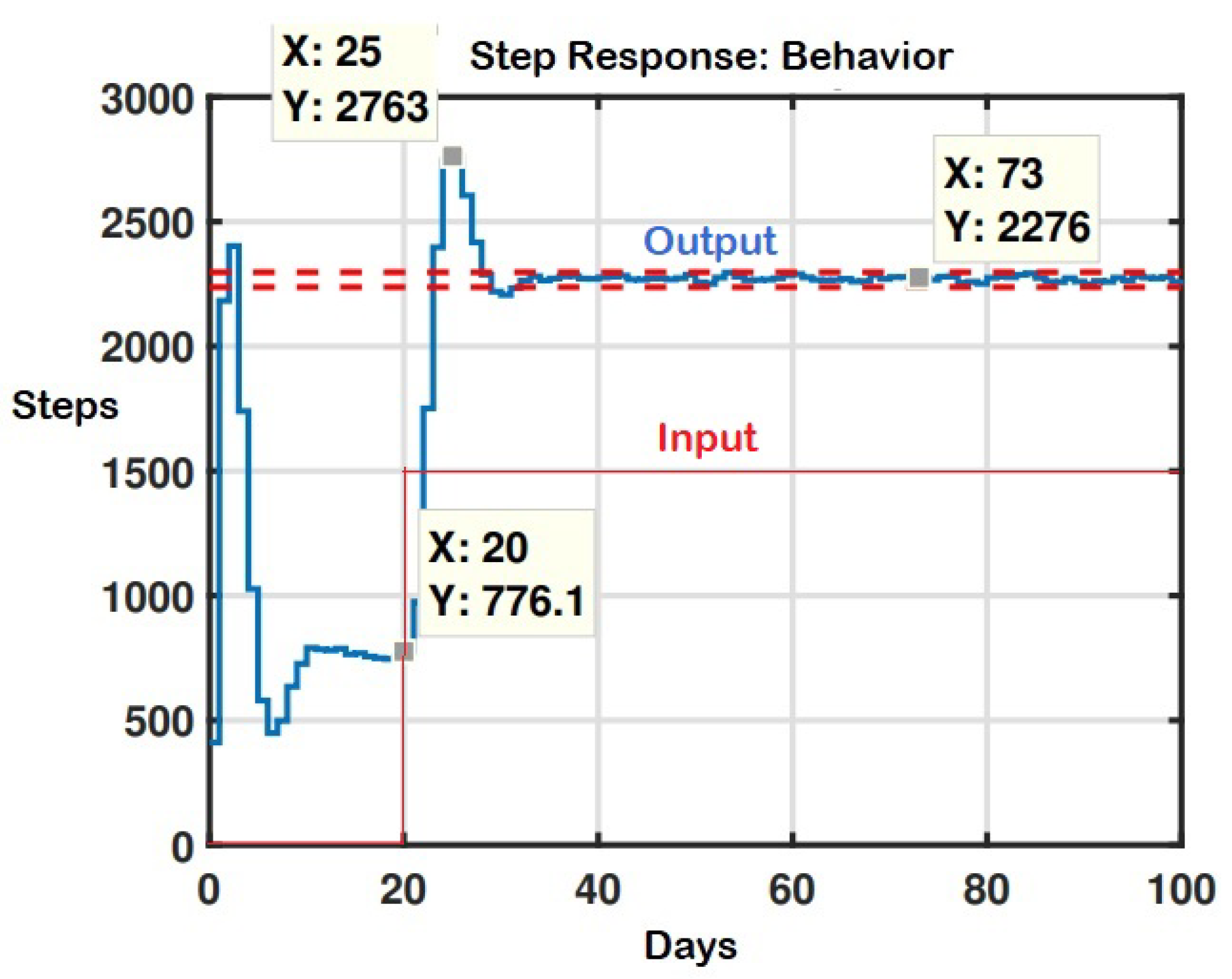
The proper selection of controller parameters (tuning) can be estimated by analyzing the open-loop step response of the proposed behavioral interventions. The choice of suitable values for these parameters is important because they affect not only the controller’s performance but also the computational complexity of the MPC algorithm, which solves an optimization problem online at each time step. Analyzing an open-loop step response is important because it provides information about the dynamic behavior of a system. It allows us to observe the system’s response to a sudden change in its input and measure its performance in terms of characteristics such as rise time, settling time, overshoot, and steady-state error. This information is crucial for obtaining specifications of the system (human behavior) and tuning the controller parameters to achieve desired performance. By analyzing the open-loop step response, we can gain insights into the system’s stability, transient response, and steady-state behavior, which are all essential for designing and implementing control systems. Given the aim of reaching 10,000 steps daily, our approach to conducting the open-loop test involves setting a target of 1500 steps per day for the model and observing the point at which the system attains stability, as indicated in Figure 6. Based on the system’s stabilization from day 20 onwards, calculations are made for the dynamic specifications of the performed step response.

From this, some specifications and parameters of the system are calculated: percent overshoot ($\%OS$), damping ratio ($\zeta$), natural frequency (${\omega }_n$), and rise time ($T_r$). Rise time is the time required for the system output to reach and maintain a percentage of its final value, typically 90%. It is an important characteristic of a system’s response because it indicates how quickly the system can respond to changes in its input. A shorter rise time indicates a faster response and better performance. See Equations (12)–(15).

$$\%OS=\frac{2763-2276}{2276-776.1}\times 100=32.46\%,$$

(12)

$$\zeta =\frac{-ln(\%OS/100)}{\sqrt{{\pi }^2+{\left(ln(\%OS/100)\right)}^2}}=0.337,$$

(13)

$${\omega }_n=\frac{\pi }{T_p\sqrt{1-{\zeta }^2}}=0.67(rad/day),$$

(14)

$$T_r=\frac{\pi -co{s}^{-1}\left(\zeta \right)}{{\omega }_n\sqrt{1-{\zeta }^2}}=1.99\left(days\right).$$

(15)

The sampling time parameter ($T_s$) is the rate at which data are sampled. This time is determined based on two considerations: limiting the number of samples to 20 during the rise time to avoid computational overload, and following Nyquist’s theorem, which requires sampling a periodic signal at more than twice the highest frequency component of the signal [24]. See Equations (16) and (17).

$$\begin{array}{cc}\hfill T_s& >\frac{T_r}{20}\hfill \\ \hfill T_s& >\frac{1.99}{20}\hfill \\ \hfill T_s& >0.099\left(days\right),\hfill \end{array}$$

(16)

$$\begin{array}{cc}\hfill {\omega }_s& >2{\omega }_n\hfill \\ \hfill \frac{2\pi }{T_s}& >2{\omega }_n\hfill \\ \hfill T_s& <\frac{\pi }{{\omega }_n}\hfill \\ \hfill T_s& <4.69\left(days\right).\hfill \end{array}$$

(17)

Thus, given $0.099<T_s<4.69$, a value of $T_s=1$ is recommended.

Selecting a prediction horizon that covers its significant dynamics is crucial to predicting a system’s future behavior accurately. A recommended approach is to choose a value that is high enough to capture the relevant dynamics but not too high to introduce unnecessary delay [13]. Based on the calculation of the sampling time, it is recommended to use a prediction horizon of 20 to 40 samples in order to cover the transient response of the open-loop system. A prediction horizon parameter value of 30 was selected. Choosing a very large control horizon only increases computational complexity. The control horizon was chosen to be less than (or equal to) the prediction horizon [25]. Thus, the value of the control horizon parameter was selected to be equal to 10.

Finally, the parameters shown in

Table 2. Tuning of model predictive control. Sample time is set equal to 1 to limit samples to 20 during rise time and to follow Nyquist’s theorem. A prediction horizon of 20 to 40 samples is recommended. Therefore, a value of 30 is chosen. A control horizon equal to 10 is selected, as this value is typically less than (or equal to) the prediction horizon [25].

Parameter	Value
Sample time	1
Prediction Horizon	30
Control horizon	10

were selected, and a maximum number of 15,000 steps as the daily goal was chosen. Additionally, considering that 10 points correspond to one cent of a US dollar, a maximum daily limit of 5000 points, corresponding to USD 5 as a reward, was established.

3.2. MPC Close Loop Structure

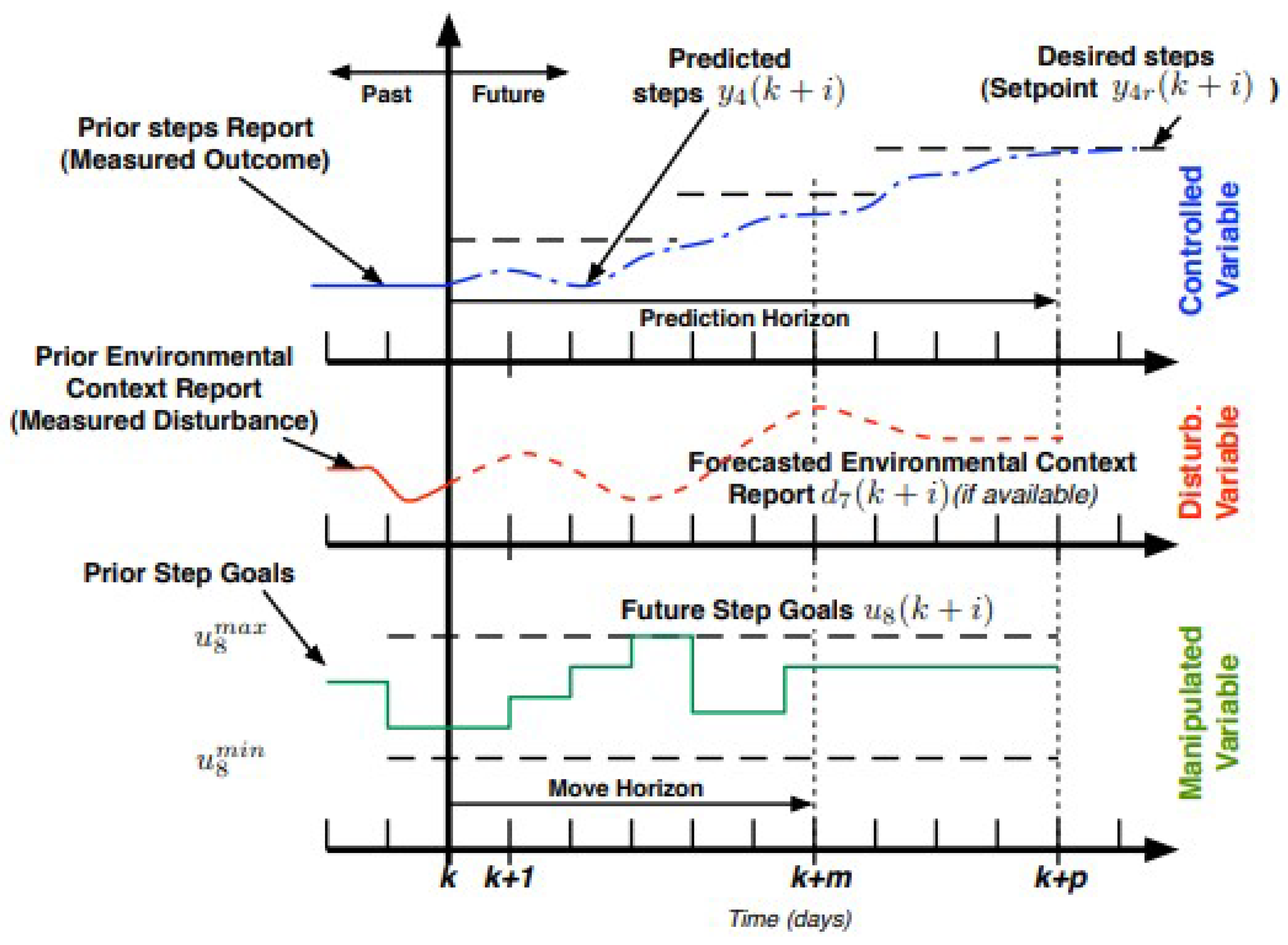
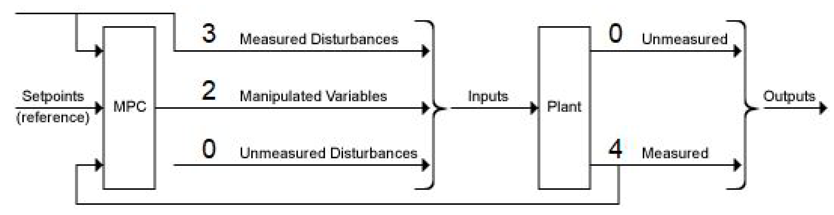
MPC uses a system model to predict behavior (e.g., the number of steps). It handles MIMO systems (Multiple-Input Multiple-Output) with interactions between inputs and outputs. The goal is to find the optimal control action that minimizes a cost function subject to constraints. Quadratic Programming (QP) is a mathematical optimization technique that aims to find the optimal solution to a given problem by minimizing or maximizing an objective function subject to certain constraints. QP involves the use of mathematical models and algorithms to optimize a specific objective function while satisfying a set of constraints. Thus, QP was used to determine the best control input at each time step, to achieve optimal performance while adhering to the system’s constraints. The strategy is known as a receding horizon control strategy, where only the first calculated moves are applied at each instant and the process is repeated to obtain new control moves. 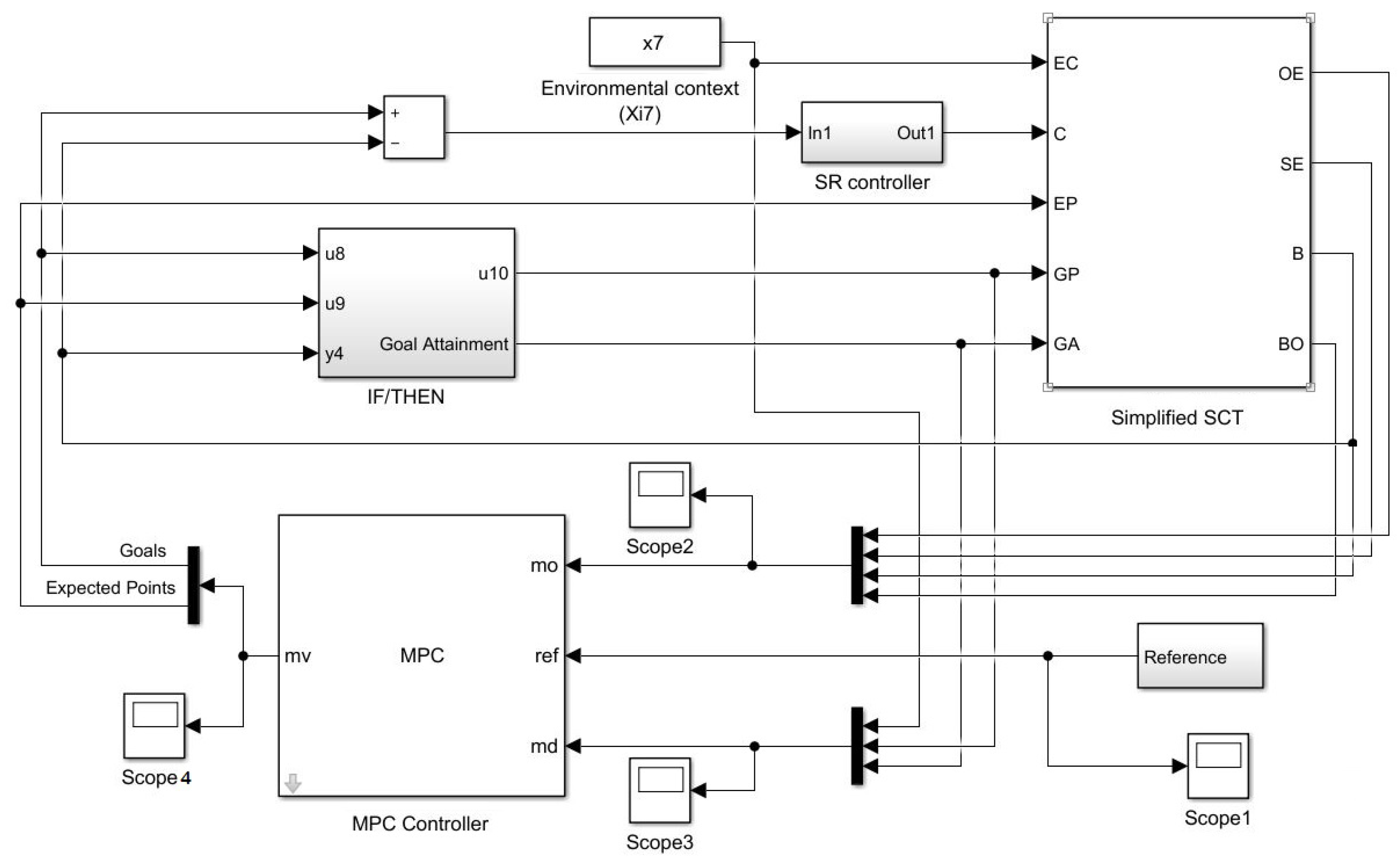This strategy is shown in Figure 7. The MPC structure used in this project is shown in Figure 8. The layout of the project ecosystem implemented in MATLAB ^® is shown in Figure 9. Some abbreviations used in this figure are explained in

Table 3. Bandura’s simplified SCT model inputs and outputs.

Symbols	Inputs	Acronym
${\xi }_7$	Environmental context	EC
${\xi }_8$	External Cues	C
${\xi }_9$	Expected points	EP
${\xi }_{10}$	Granted points	GP
${\xi }_{11}$	Goal attainment	GA
Symbol	Outputs	Acronym
${\eta }_2$	Outcome expectancies	OE
${\eta }_3$	Self-efficacy	SE
${\eta }_4$	Behavior	B
${\eta }_5$	Behavioral outcomes	BO

.

At each time instant (t), the controller uses previous system information and its states, current demands, and control actions to forecast the system outcome for the prediction horizon. Based on this, it calculates a sequence of future control actions for the control or move horizon by solving an optimization problem using cost functions from Equations (18) and (19).

$$\mathit{J}\left(z_k\right)={\mathit{J}}_y\left(z_k\right)+{\mathit{J}}_u\left(z_k\right)+{\mathit{J}}_{\Delta u}\left(z_k\right)+{\mathit{J}}_{\epsilon }\left(z_k\right)$$

(18)

$$z_k^T=\left[u{\left(k\right|k)}^{T}u{(k+1|k)}^T...u{(k+p-1|k)}^T{\epsilon }_k\right],$$

(19)

where J${}_i\left(z_k\right)$ are the partial cost functions, $z_k$ is the quadratic programming ($QP$) decision, and slack variable ${\epsilon }_k$ (dimensionless) represents the deviation of system state variables from their setpoints at each control interval in control systems.

$${\mathit{J}}_y\left(z_k\right)=\sum _{j=1}^{n_y}\sum _{i=1}^p{\left\{\frac{w_{i,j}^y}{s_j^y}\left[r_j(k+i|k)-y_j(k+i|k)\right]\right\}}^2,$$

(20)

where:

• k is the current control interval;
• p is the prediction horizon (number of intervals);
• $n_y$ is the number of plant output variables;
• $y_j(k+i|k)$ is the predicted value of the jth plant output at the $i-$th prediction horizon step;
• $r_j(k+i|k)$ is the reference value for the jth plant output at the ith prediction horizon step;
• $s_j^y$ is the scale factor for the jth plant output;
• $w_{i,j}^y$ is the tuning weight for the jth plant output at the ith prediction horizon step (dimensionless).

The values $n_y$, p, $s_j^y$, and $w_{i,j}^y$ are constant controller specifications. The controller receives $r_j(k+i|k)$ for the entire prediction horizon and uses the state observer to predict the plant outputs, $y_j(k+i|k)$, which depend on manipulated variables (MV) adjustments $\left(u_k\right)$ (goals ($u_8$) and expected points ($u_9$)), measured disturbances (MD), and state estimates. At interval k, the state estimates and MD values are available. Therefore, $J_y$ is a function of $z_k$ only.

The second cost function is:

$${\mathit{J}}_u\left(z_k\right)=\sum _{j=1}^{n_u}\sum _{i=0}^{p-1}{\left\{\frac{w_{i,j}^u}{s_j^u}\left[u_j(k+i|k)-u_{j,target}(k+i|k)\right]\right\}}^2,$$

(21)

where:

• $n_u$ is the number of MV;
• $u_{j,target}(k+i|k)$ is the target value for jth MV at the ith prediction horizon step;
• $s_j^u$ is the scale factor for the jth MV;
• $w_{i,j}^u$ is the tuning weight for the jth MV at the ith prediction horizon step (dimensionless).

The values $n_u$, p, $s_j^u$ and $w_{i,j}^u$ are constant controller specifications. The controller receives $u_{j,target}(k+i|k)$—values for the entire horizon. The controller uses the state observer to predict the plant outputs. Thus, $J_u$ is a function of $z_k$ only.

An MPC controller uses the subsequent scalar performance metric to suppress the movement of manipulated variables (see Equation (22)),

$${\mathit{J}}_{\Delta u}\left(z_k\right)=\sum _{j=1}^{n_u}\sum _{i=0}^{p-1}{\left\{\frac{w_{i,j}^{\Delta u}}{s_j^u}\left[u_j(k+i|k)-u_j(k+i-1|k)\right]\right\}}^2$$

(22)

and the partial cost function for the slack variable ${\epsilon }_k$ (see Equation (23)). In practical applications, constraint violations can sometimes be inevitable. Soft constraints ensure a feasible QP solution even under such conditions. An MPC controller utilizes a slack variable, ${\epsilon }_k$, which is non-negative (greater than or equal to zero) and dimensionless, to measure the worst-case constraint violation.

$${\mathit{J}}_{\epsilon }\left(z_k\right)={\rho }_{\epsilon }{\epsilon }_k^2,$$

(23)

where:

• ${\epsilon }_k$ is the slack variable at control interval k (dimensionless);
• ${\rho }_{\epsilon }$ is the constraint violation penalty weight (dimensionless).

The slack variable ${\epsilon }_k$ represents the amount by which the system state variables can deviate from their setpoints at each control interval. The value of ${\epsilon }_k$ is used to ensure that the constraints are satisfied within the given tolerance levels. On the other hand, the weight assigned to the constraint violation penalty, ${\rho }_{\epsilon }$, is a scalar value that determines the trade-off between achieving a lower cost function and satisfying the constraints. A higher value of ${\rho }_{\epsilon }$ indicates a greater penalty for violating the constraints, which can lead to a more conservative controller.

MPC constraints are limited as shown below.

$$\begin{array}{c}\hfill y_{min}\le \frac{y_j(k+i|k)}{s_j^y}\le y_{max},i=1:p,j=1:n_y\\ \hfill u_{min}\le \frac{u_j(k+i-1|k)}{s_j^u}\le u_{max},i=1:p,j=1:n_u\\ \hfill \Delta u_{min}\le \frac{\Delta u_j(k+i-1|k)}{s_j^u}\le \Delta u_{max},i=1:p,j=1:n_u,\end{array}$$

(24)

where:

$$\begin{array}{c}\hfill y_{min}=\frac{y_{j,min}\left(i\right)}{s_j^y}-{\epsilon }_k{V}_{j,min}^y\left(i\right)\\ \hfill y_{max}=\frac{y_{j,max}\left(i\right)}{s_j^y}+{\epsilon }_k{V}_{j,max}^y\left(i\right)\\ \hfill u_{min}=\frac{u_{j,min}\left(i\right)}{s_j^u}-{\epsilon }_k{V}_{j,min}^u\left(i\right)\\ \hfill u_{max}=\frac{u_{j,max}\left(i\right)}{s_j^u}+{\epsilon }_k{V}_{j,max}^u\left(i\right)\\ \hfill \Delta u_{min}=\frac{\Delta u_{j,min}\left(i\right)}{s_j^u}-{\epsilon }_k{V}_{j,min}^{\Delta u}\left(i\right)\\ \hfill \Delta u_{max}=\frac{\Delta u_{j,max}\left(i\right)}{s_j^u}+{\epsilon }_k{V}_{j,max}^{\Delta u}\left(i\right).\end{array}$$

(25)

Here, $V_j$ parameters correspond to the Equal Concern for Relaxation parameter (ECR), which specifies the relative importance of satisfying constraints versus achieving performance goals in a control problem. They are dimensionless controller constants analogous to the cost function weights and used for constraint softening (zero implies a hard constraint). A more significant positive ECR value means that the controller is willing to compromise the satisfaction of the constraint to achieve the goals.

• ${\epsilon }_k$ is a scalar QP slack variable (dimensionless) used for constraint softening;
• $s_j^y$ is a scale factor for the jth plant output;
• $s_j^u$ is a scale factor for the jth MV;
• $y_{j,min\left(i\right)}$, $y_{j,max\left(i\right)}$ are the lower and upper bounds for the jth plant output at the ith prediction horizon step;
• $u_{j,min\left(i\right)}$, $u_{j,max\left(i\right)}$ are the lower and upper bounds for the jth MV at the ith prediction horizon step;
• $\Delta u_{j,min\left(j\right)}$, $\Delta u_{j,max\left(i\right)}$ are the lower and upper bounds for the jth MV increment at the ith prediction horizon step.

Due to the substantial correlation between higher daily step counts and lower mortality risk, a recommended target of 10,000 steps per day has been established [26].

As mentioned before, a maximum number of 15,000 steps as the daily goal was chosen. Furthermore, a daily cap of 5000 points was set, which equates to a reward of USD 5, given that 10 points are equivalent to one cent. These constraints are indicated in

Table 4. MPC constraints. Goals ($u_8$) and expected points ($u_9$) are the manipulated variables (MV). $\Delta u_i$ refers to the change in the signal i between two consecutive time instances.

Parameter	Min	Max	Unit
$u_8$	0	15,000	(steps/day)
$u_9$	0	5000	(points/day)
$\Delta u_8$	unconstrained		(steps/day)
$\Delta u_9$	unconstrained		(points/day)

.

In an MPC controller design, the selection of the weights must be chosen to favor or disfavor the variability of the MVs, their rate, and the variability of the outputs. The selected weights for the MPC are shown in

Table 5. MPC weights. Taking into account the economic factor which is critical for the project, the controller will try to penalize abrupt values of offered reward points ($u_9$) for which the weight of 1 is assigned. The weight of the daily step goal ($u_8$) was set to zero. The weights assigned to $\Delta u_8$ and $\Delta u_9$ are both 0.1, indicating that those variables are not considered significant. The weight of the output variable ${\eta }_4$ is also equal to 1 since that variable, which corresponds to the behavior, is the one to be regulated, leaving the other outputs to vary freely (other output weight = 0).

Parameter	Weights				Unit
$u_8$	0				dimensionless
$u_9$	1
$\Delta$$u_8$$\Delta$$u_9$	0.1
Output Variables	${\eta }_2$ = 0	${\eta }_3$ = 0	${\eta }_4$ = 1	${\eta }_5$ = 0	dimensionless

.

4. Results Analysis

It is essential to use accurate system parameters when designing and testing a control system to ensure that it performs as expected and achieves the desired control objectives. Thus, an identification procedure with the data from the “hypothetical model” was performed to obtain a linear state-space variable model. This discrete model was then used to design an MPC controller that considers the actual system dynamics. However, to test the controller the “hypothetical model” was used. This led to a difference between the identified parameters used for the MPC design and the system’s parameters used for simulation, similar to what may occur in a real scenario.

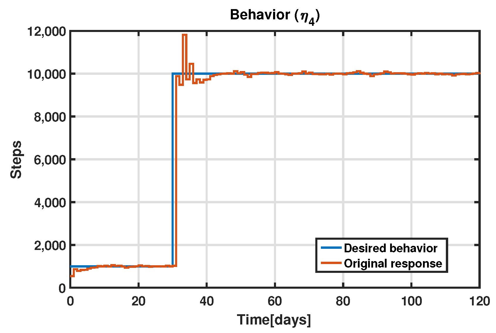
The proposed controller was tested and the following results were obtained (Figure 10). The results from day 30 to day 120 are shown. During the first month, an initial desired behavior of 1000 daily steps was set.

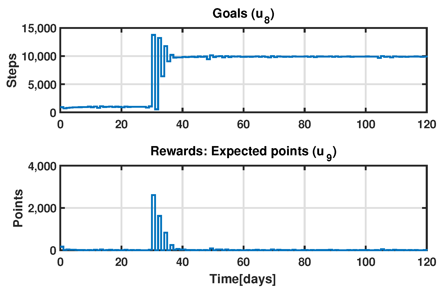
The response of the manipulated variables (i.e., goals ($u_8$) and expected points ($u_9$)) is shown in Figure 11, demonstrating the successful achievement of the constraints considered in the MPC design. Since the weight of the expected points was set to 1 (the highest level of importance), the signal tends to decrease over time. On the other hand, the weight of the goals was set to 0, resulting in an increase and stabilization of the signal at a steady-state value of around 10,000 steps.

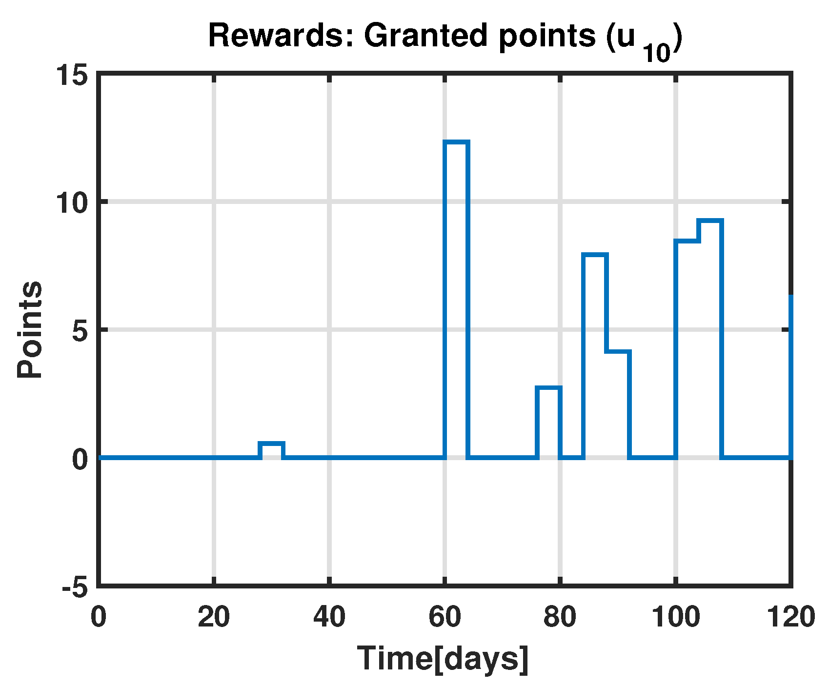
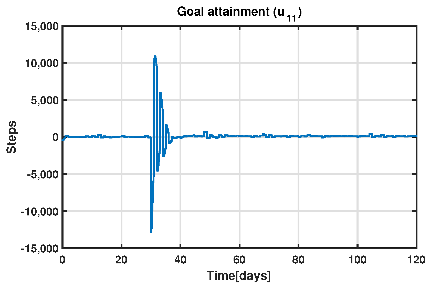
In Figure 12 and Figure 13, the other input variables (granted points ($u_{10}$) and goal attainment ($u_{11}$)) are shown. It is noticeable that the number of granted points in Figure 12 was lower than the number of expected points in Figure 11. Meanwhile, the goal attainment signal in Figure 13 shows that, for the majority of the experiment, the number of daily steps taken surpassed the proposed goal.

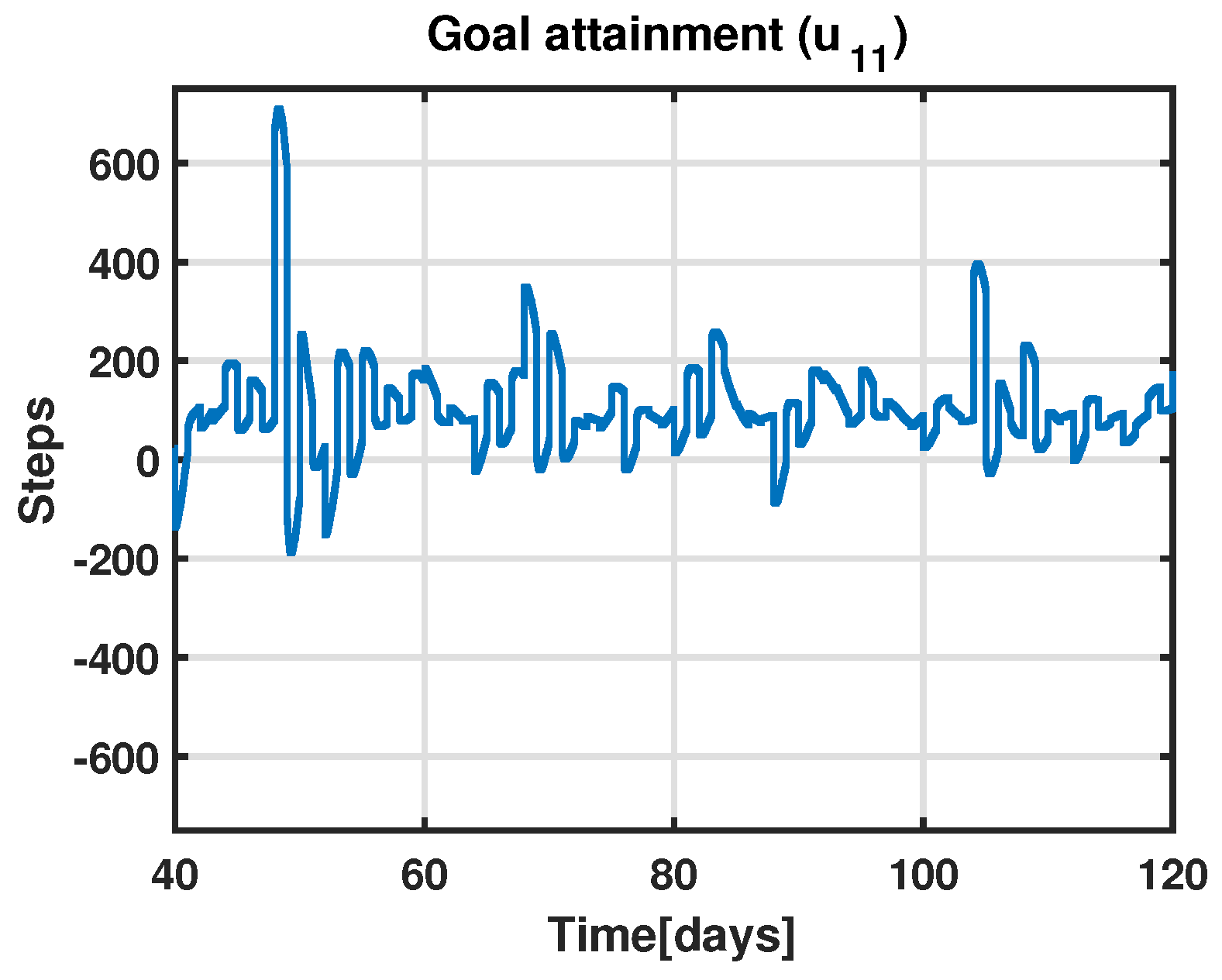
In Figure 14, the steady state of the goal attainment signal is shown. It can be observed that most of the time this signal has positive values, which indicates that the number of daily steps is greater than the set goal. Goal attainment positively affects behavior through the auto-efficacy inventory as demonstrated through the fluid analogy of the SCT model.

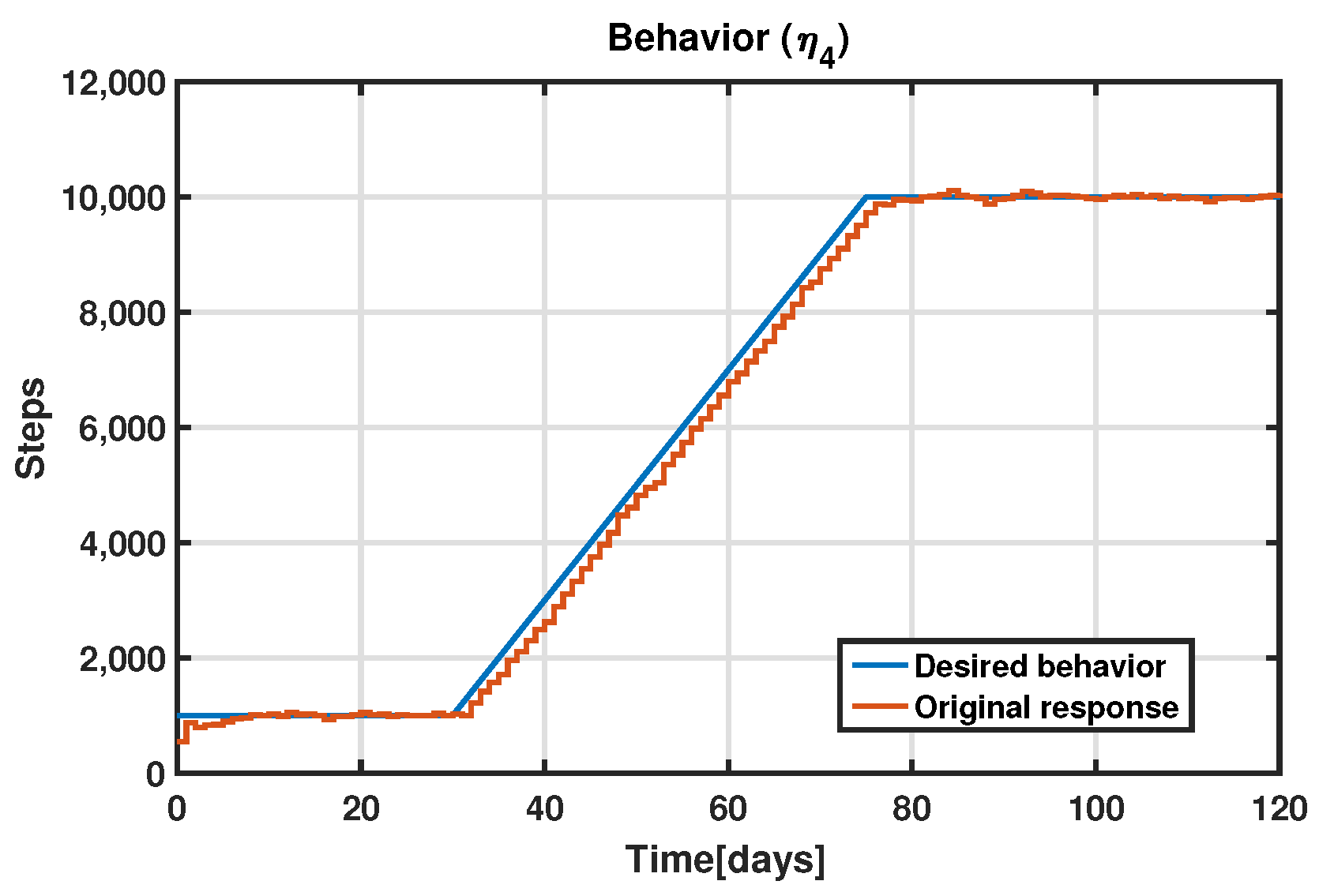
The designed controller achieves the desired behavior even though there is a mismatch between the model used for the MPC design and the model used for the simulation. Thanks to the robust control ideas of this type of controller, the difference between those models does not affect the system’s performance. Only a few points were needed as rewards to achieve the desired behavior. A ramp test was also performed to examine the dynamic performance of a system by evaluating how it reacts to a gradually varying input signal. The results of this progressive approach can be observed in Figure 15. It can be observed that the output tracks the reference input, achieving zero steady-state error. This input type is suggested for the experiment to avoid abrupt changes in the output with the step input.

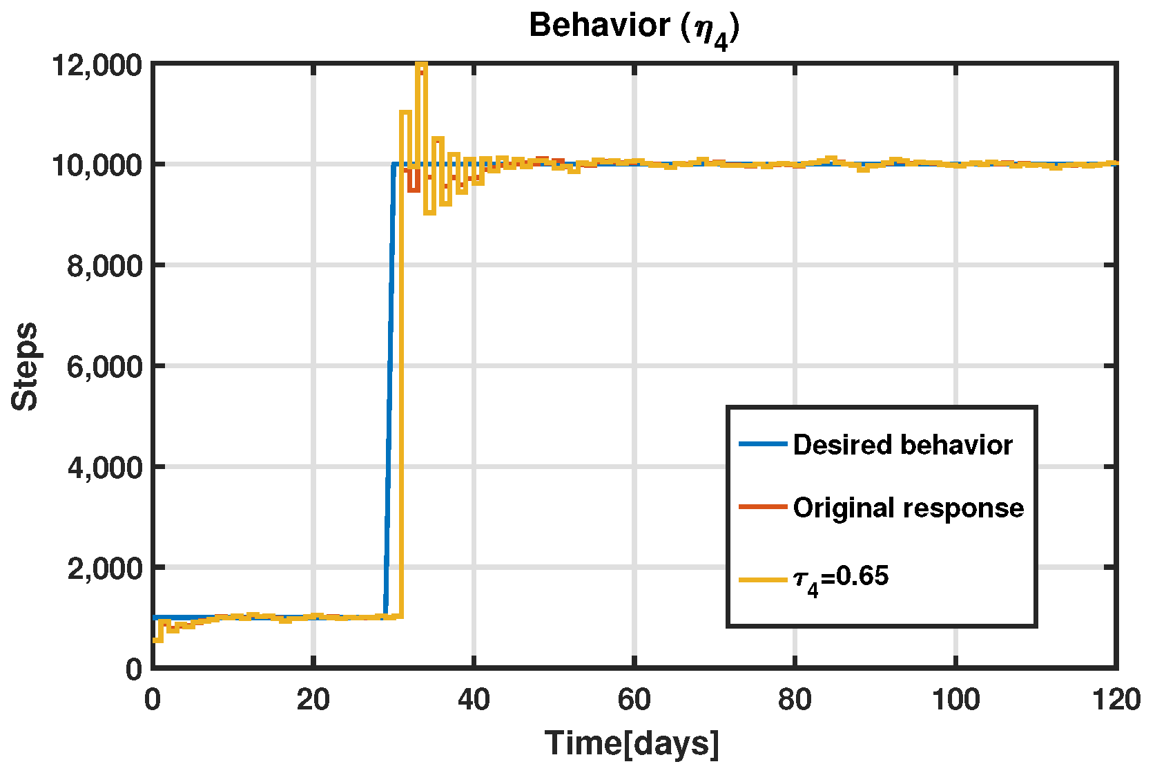
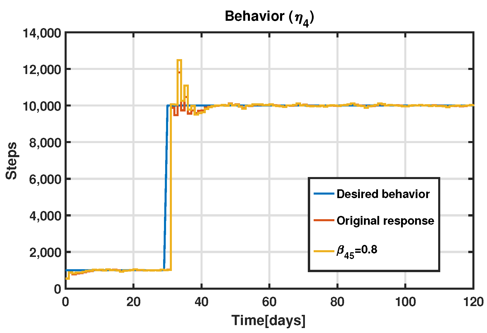
To further demonstrate the performance of the designed controller, two parameters that directly affect behavior were modified; the values were arbitrarily selected. In the first scenario, the time constant ${\tau }_4$ was modified from 0.8 to 0.65 days. Figure 16 shows the original and modified responses. In the second scenario, the input coefficient from the behavior inventory ${\beta }_{45}$ was modified from 0.5 to 0.8; the obtained results are shown in Figure 17. In both scenarios, it can be observed that the obtained responses do not suffer any significant change compared to the system response without the parameter modification.

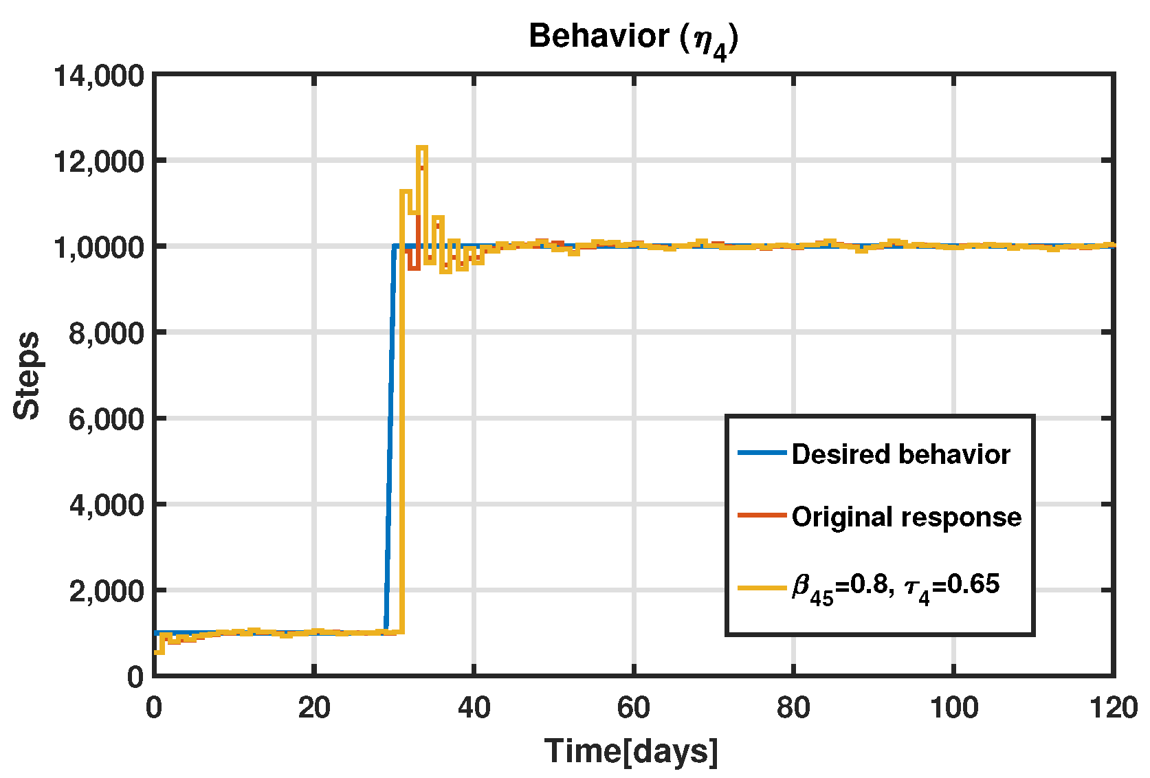
The results obtained from varying both ${\tau }_4$ and ${\beta }_{45}$ simultaneously are shown in Figure 18. In the three scenarios, it can be observed that the steps tracking is maintained, thus zero steady-state error is achieved even though there is a mismatch between the identified model, which was used for the MPC design, and the hypothetical model used for the simulation, which also had some of its parameters modified.

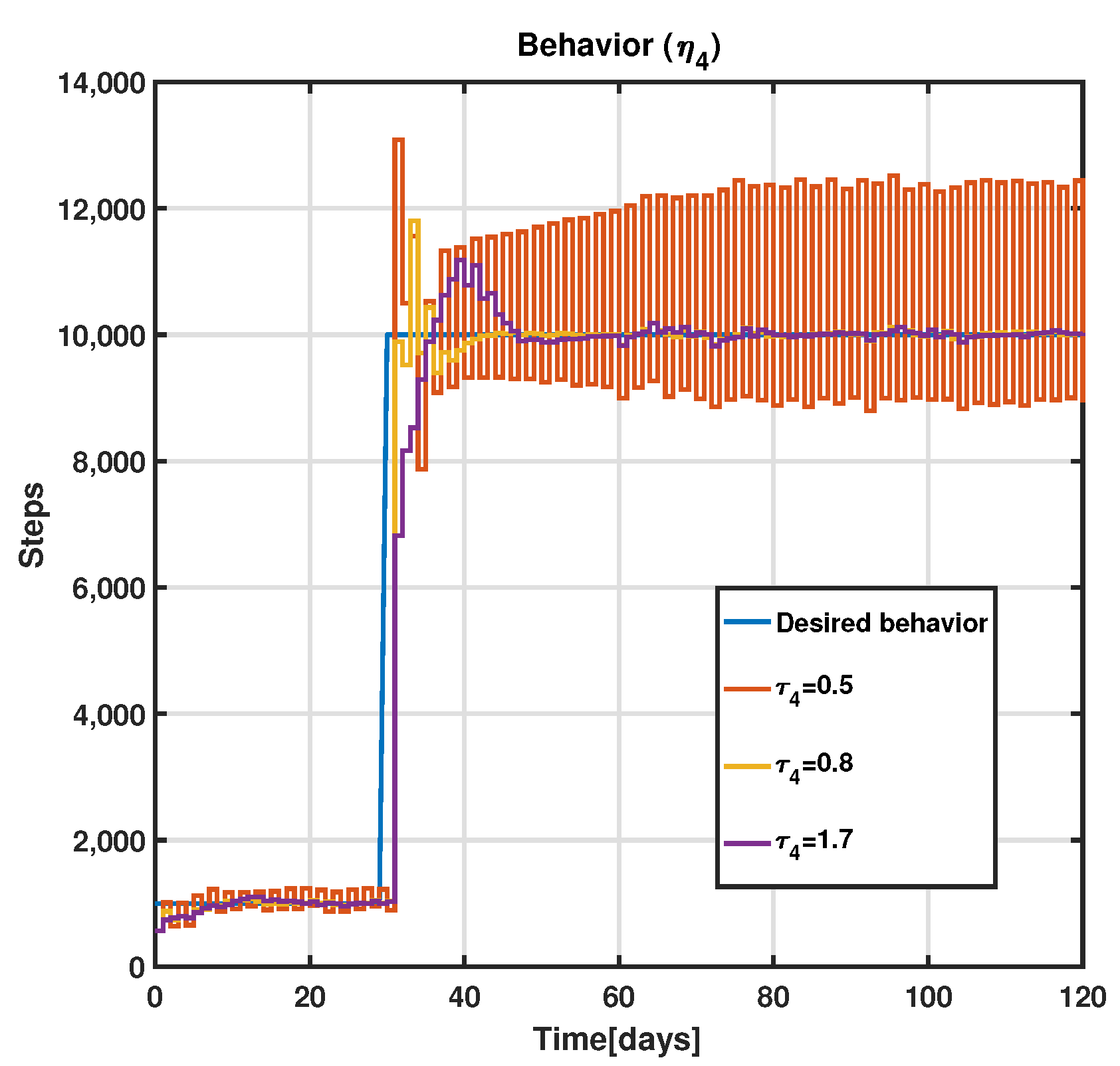
The effect of the time constant parameter ${\tau }_4$ is significant for the system’s performance. A time-constant sweep was performed via simulation. The results obtained from the simulation for the minimum and maximum tested values, as well as for the original value (${\tau }_4=0.8$) are shown in Figure 19. It should be noted that the controller responds better when the time constant is increased from its original value than when it is decreased. When the time constant decreases, the system tends to become unstable.

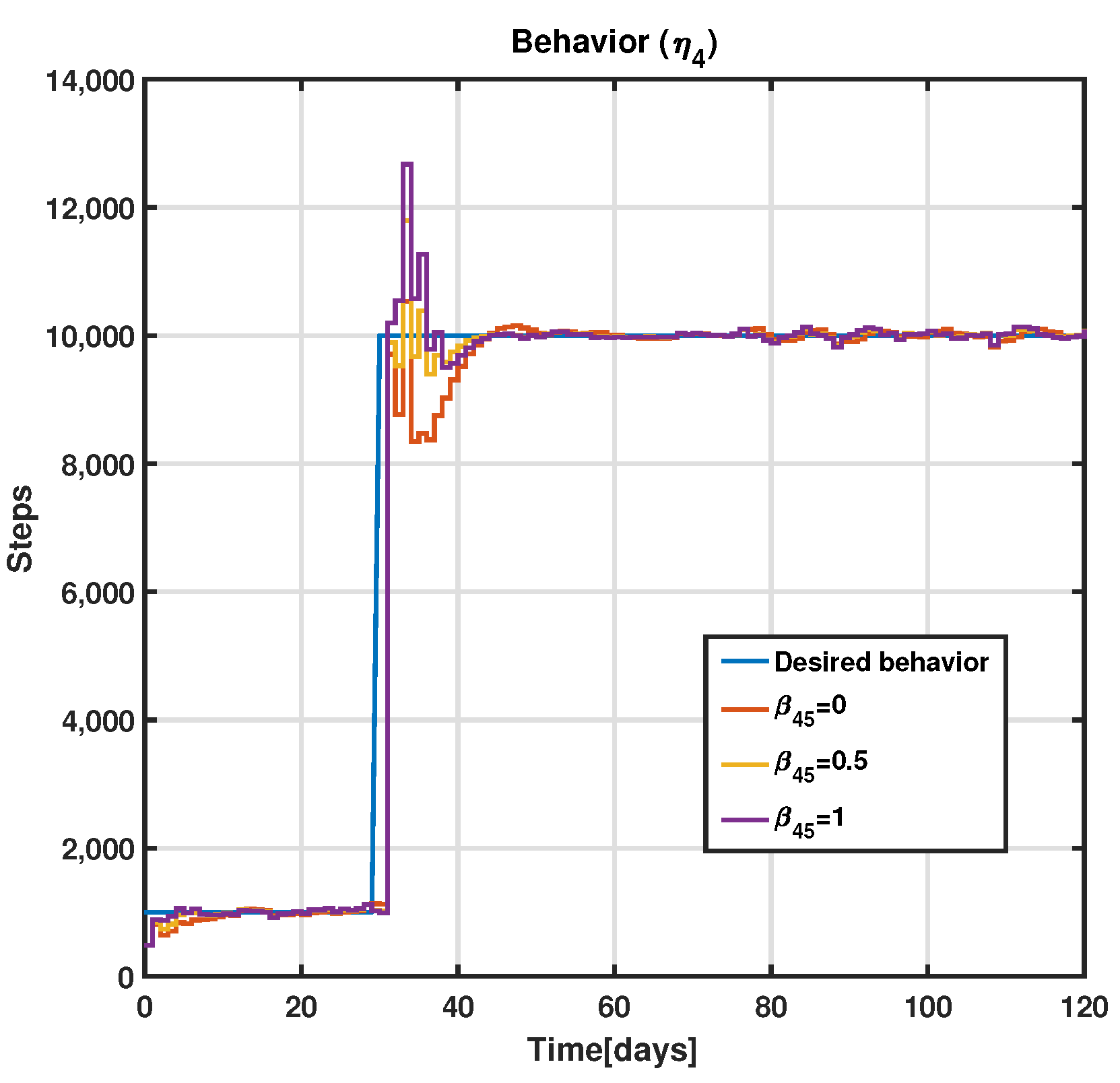
A sweep was conducted for the parameter value of $\beta$, with the limitation that it can only take values between 0 and 1. The results obtained from the simulation with all arbitrarily considered values are shown in Figure 20. The settling time is approximately the same in the three scenarios. However, the percentage overshoot is affected by the parameter variation but the zero steady-state error is still achieved. The time constant parameter ${\tau }_4$ is more sensitive (meaning it has a greater impact on the stability of the system) than the input coefficient ${\beta }_{45}$.

An analysis of the obtained results is presented below, along with relevant comments and requisite considerations, while acknowledging that this is an approximation of a complex system such as human behavior.

Despite the limitations of the mathematical modeling of human behavior, initial estimates of the MPC controller’s parameters were made based on the model obtained. Open-loop tests were conducted to establish the natural and uncontrolled response of the model, followed by closed-loop tests to evaluate the system’s response to gradual and continuous changes in input. The controller successfully regulated both step and ramp signals, although the step response showed a relatively high overshoot. Implementing saturation-limiting elements could address this issue.

Finally, closed-loop tests were conducted for different scenarios and the controller was effective in absorbing variations in sensitivity levels depending on the parameter being varied. We should note that the time constant parameter ${\tau }_4$ appears to have a considerably more significant impact on the stability of the system compared to the input coefficient ${\beta }_{45}$. This suggests that it exhibits a higher level of sensitivity concerning the stability of the system.

5. Conclusions and Future Work

In previous work co-authored by some of the present study’s authors, a model was obtained relying on secondary data focused on interventions for physical inactivity problems [9]. However, the earlier model did not take into consideration some critical aspects needed for the proposed behavioral interventions. In the present study, a new hypothetical model was proposed including information obtained from the initial secondary data modeling, supplemented with additional parameters obtained from previous experiments and personal experiences to include all the inputs and outputs needed for the proposed behavioral intervention.

This hypothetical model was simulated under realistic conditions to provide data for system identification; the model obtained as a result of this process was used for the MPC design. As frequently seen in practical control scenarios, some of the parameters of the hypothetical model differ from the parameters of the identified linear model causing a model mismatch. Another factor contributing to model mismatch is the non-linearity of the hypothetical system and the fact that each person’s state represents a different set of those parameters.

Because this model represents human behavior using Bandura’s Social Cognitive Theory and fluid analogy, a mismatch will exist between the person’s behavior, the model output, and the identified system output. This leads to the need for a model-based controller that is able to absorb the model mismatches. The MPC control strategy meets these requirements and was demonstrated to be suitable for the non-linear behavioral intervention model. This work presented the results from the proposed adaptive MPC Control Design applied to a non-linear behavioral intervention model.

Simulations demonstrated that the MPC controller could maintain zero steady-state error and similar settling times even if a critical parameter of the behavior inventory was modified. Additionally, because it is possible to set weights and constraints using this control strategy, the number of points granted as a reward was low, which is important for the economic aspect of this kind of intervention. A settling time of approximately 10 days was achieved. However, this value is not feasible in a real-life situation because other aspects need to be taken into account that the model does not. For example, in this case, if someone is able to achieve the goal within 10 days, he/she is probably able to succeed without the need for additional rewards. This is a case of someone who is likely a young athlete, and therefore is outside the target group of interest.

As future work, a validation test for the mathematical models created through system identification, which is the process of building mathematical models of dynamic systems based on observed data, should be performed. A reliable model is needed for a good MPC performance, hence system identification is a fundamental undertaking prior to the MPC design. The duration of the experiment is critical if it is performed in real-time and not simulated, so a test monitoring procedure should also be performed during the online identification of the parameter values carried out to improve the reliability of the obtained model.

Due to the nature of the system, each person represents a different set of parameters. Additionally, for a given person, this set of parameters can change as a function of that person’s state (mental, physical, or environmental). Therefore, a multiple MPC design is highly recommended. This controller could include different models that represent different states of a given person and switch the controller parameters, weights, and constraints used depending on their current and past states.