Analysis and Design of Nonlinear Tuned Mass Damper Based on Complex Variable Averaging Method

Featured Application

The use of this analytical method can improve the damping performance of tuned mass dampers, which has a certain reference value in the subsequent study of TMD nonlinear characteristics, and the analytical method has some significance for improving the efficiency in practical engineering.

Abstract

As one of the most representative passive control devices, tuned mass dampers (TMDs) are widely used in civil engineering, aerospace, machinery, and other fields, after years of research and improvement. However, due to their large displacement and the use of a limiting device, they inevitably exhibit some nonlinear characteristics in practical engineering applications. This nonlinearity is often ignored; however, neglecting it in the design process can adversely affect the control performance. Therefore, considering the nonlinearity of a TMD while designing TMD parameters can make the calculation results closer to reality and benefit the structural design. In this paper, we derived the approximate analytical solution of TMD amplitude using the complex variable averaging method by considering the nonlinearity generated by a TMD in the vibration process. Theoretical optimal design parameters were obtained by analytical comparison, and we compared the computational time consumption of this method and the numerical method. The results showed that the optimized parameters of the TMD obtained by nonlinear design possessed a good vibration reduction effect both before and after the TMD generated nonlinear characteristics. Additionally, the complex averaging method generated frequency response curves tens of times faster than the numerical method.

1. Introduction

Vibration is a physical phenomenon that is prevalent in nature and human social activities, and the harm it causes cannot be ignored [1]. In the field of civil engineering, the force state of building structures is very complex, and vibrations caused by unpredictable natural disasters and other phenomena can pose a serious threat to the structure, leading to huge casualties and property damage, such as building collapses caused by earthquakes [2] and bridge fractures caused by resonance due to wind loads [3]. Therefore, the effective control of vibrations is imperative [4,5]. Structural control techniques are an effective means of reducing the adverse effects of vibrations, and control devices are divided into three main types: active, passive, and semi-active control devices [6]. The main difference is whether the device requires external energy input. The use of active control in engineering is greatly limited due to the additional controls required and the high cost of use. Passive control devices are simple and basic in design, with the advantages of low cost, good stability, and no external energy input. Among these, tuned mass dampers (TMDs) are the most representative and most widely used in practical applications.

TMDs originated in 1909 when Frahm invented a dynamic vibration absorber (DVA) in 1911 [7]. However, the DVA was originally designed without damping, which resulted in poor control in some frequency bands. Den Hartog improved the DVA by introducing damping, which significantly improved the vibration reduction and established the concept of a TMD. After this, Den Hartog optimized the TMD and provided optimized formulas for the frequency ratio and damping ratio [8]. Setareh et al. determined the optimal damping of the TMD based on the integral modal method [9].

TMDs have been successfully applied in many projects and have proven their effectiveness. The Sydney Television Tower was the first building to use a TMD as a control device. In 1970, to resist wind loads, TMDs were installed at the John Hancock Center, resulting in a 40% reduction of the impact of wind loads on the structure. Kwok used a water tank as a mass block for TMD [10] and obtained the desired control results. The Taipei 101 building in China uses a single pendulum TMD with a limiting device to control the vibration caused by external loads [11]. Meanwhile, TMDs are also widely used in the field of bridges. In 1988, a TMD system was installed on the main tower of the Akashi Kaikyo Bridge, and test experiments showed that the TMD system could increase the damping ratio of the tower from 1% to 3% when it was built [12].

TMDs absorb energy through resonance but are limited by their linearity, and they can only control a single mode, while structures usually have multiple modes. To overcome this shortcoming of TMDs, Clark proposed the multiple tuned mass damper (MTMD) in 1988 [13], which is composed of TMDs with several different dynamic characteristics. In addition, a bidirectional and homogeneous TMD (BH-TMD) was proposed by Almaz’ an et al. [14]. Roberson pointed out that the bandwidth of the controllable frequency of the damper can be effectively increased by adding nonlinearity, and the concept of a nonlinear energy sink (NES) was born [15]. To introduce nonlinearity into dampers, the most widely used are mass dampers and nonlinear stiffness dampers. Lu et al. described in detail information about plasmonic dampers [16], which provided a valuable reference for subsequent research in this field. Zhang et al. proposed a viscoelastic damper that uses a viscoelastic material to efficiently absorb the energy generated during a collision, calling it a pounding tuned mass damper (PTMD) [17]. Collision-tuned dampers [18,19] and liquid impact dampers (TLPD) [20] are also impact dampers. Starosvetsky and Starosvetsky and Gendelman studied the stressed system response (SMR) near the 1:1:1 resonance [21], investigated the conditions for the existence of the SMR, and verified its numerical results using analytical methods [22].

In reality, linearity is an ideal situation, and pure linear systems do not exist in the real world. Because of the use of large displacements or limiting devices, TMDs can have nonlinear characteristics during vibration, even if they are not considered in the design. This nonlinearity has historically been ignored in the design process, and Li and Cui confirmed that doing so can adversely affect control performance [23]. Liu et al. proposed a scheme for a hybrid control structure of NES and TMD and obtained the theoretical energy prediction equations using the multiscale method [24]. Su et al. investigated the nonlinear behavior generated by the cable under TMD control, obtained the modulation equations of the system using the multiscale method, and explored the nonlinear characteristics of the system through the modulation equations based on different key parameters [25]. Li focused on the effect of wind load on the dancing of ice-covered conductors, solved the model using an improved multiscale method, investigated the nonlinear characteristics generated by the model, and improved the TMD based on the analysis results obtained to enhance its control performance [26]. In this paper, we mainly derived the analytical approximate solution of the primary structural frequency response of a nonlinear tuned mass damper with hardening enhancement characteristics and obtained the modulation demodulation equation related to the structural amplitude. This equation can obtain the structural amplitude–frequency curve related to the TMD frequency, and we then analyzed the calculation results to obtain the optimal design parameters under the corresponding conditions and compared them with the numerical method to prove the correctness of this equation. Comparing the computational speeds of the complex variable averaging method with those of the numerical method, the results showed that the frequency response curve generated based on this analytical method was faster than that of the conventional numerical method.

The previous paragraph described the classification, working principle, history, and development of dampers. Section 2 introduces the equation of motion and its dimensionless form in this paper. Section 3 derives the approximate analytical solution for the equations of motion for this system. Section 4 verifies the accuracy of the analytical formulation using numerical methods. The optimal TMD frequency for the structure considering the nonlinear coefficients was obtained analytically, and the control performance of the TMD at this frequency was verified. After that, the control performance of linear TMD and nonlinear TMD under different design methods was compared using the obtained optimal design parameters. Section 5 compares the time of generating the amplitude–frequency response curves by the complex variable averaging method with that of the conventional numerical method, and the results show the superiority of the complex variable averaging method in terms of computational speed. Section 6 summarizes the main contents and research results of this study.

2. Equation of Motion of the System and Its Dimensionless Form

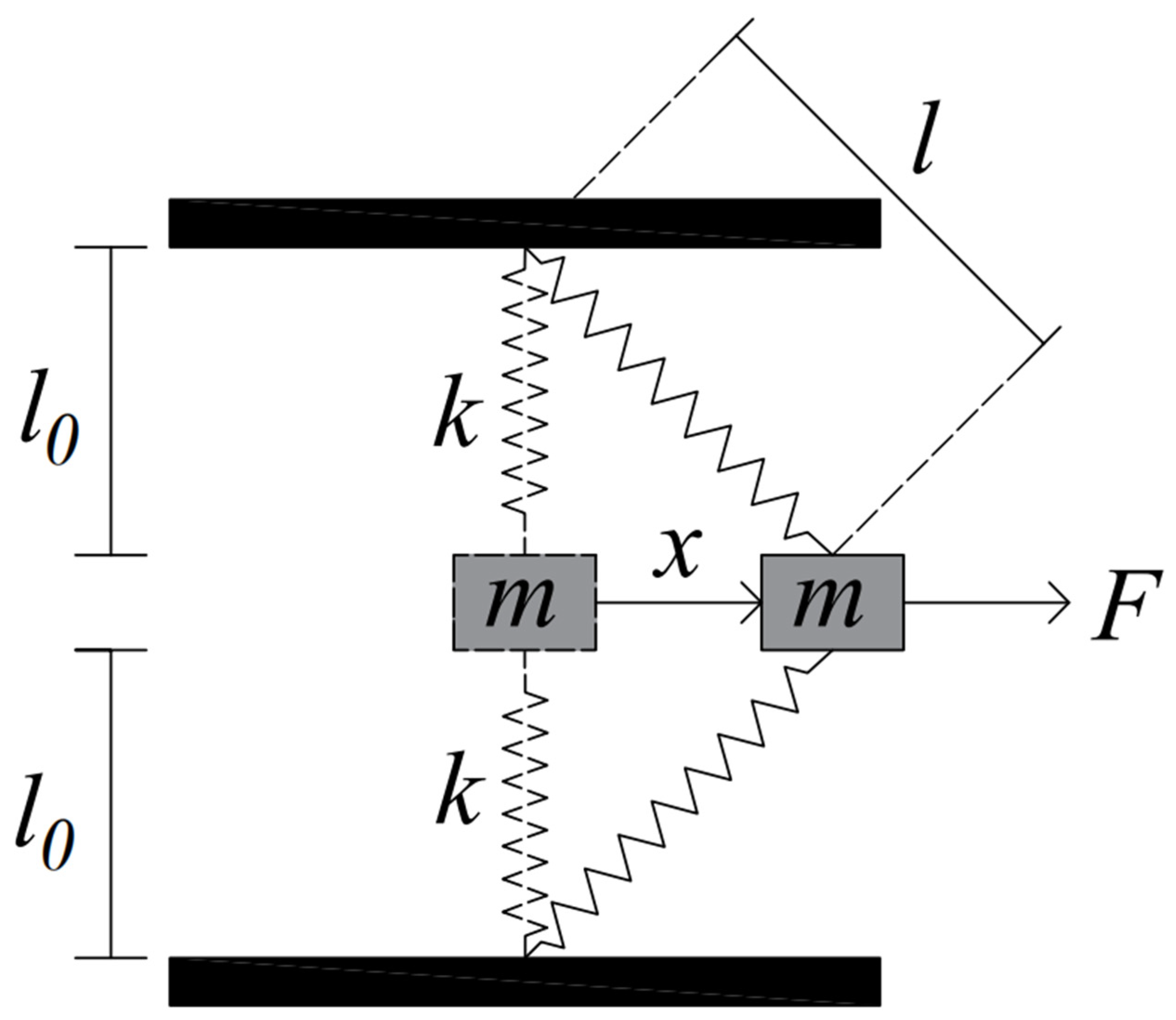
To investigate the vibration reduction performance of a nonlinear TMD, a system model was developed consisting of an ideal single-degree-of-freedom primary structure and a stiffness-geometry nonlinear TMD, with the goal of reducing the steady-state amplitude of the structure. When the primary structure is subjected to an external load, the TMD installed on it absorbs energy, and the TMD produces displacement in the horizontal direction. The spring attached to the TMD stretches and tilts, creating a geometric nonlinearity, which in turn leads to a stiffness nonlinearity in the linear spring, as shown in Figure 1.

The relationship between the restoring force f and the displacement x in the horizontal direction is described by Equation (1), where l₀ is the length of the spring at rest, l is the length of the spring after tilting, and k is the stiffness of the linear spring. The Taylor expansion is used to expand to the fifth order of x, while omitting the higher order terms. The expansion of Equation (1) results in a nonlinear restoring force, with results representing the first, third, and fifth powers of stiffness, consequently yielding Equation (2):

$$f=2kx\left(1-\frac{l}{\sqrt{x^2+l_0^2}}\right)$$

(1)

$$f\approx 2k\left(x-\frac{l_0}{l}x+\frac{l_0}{l^3}{x}^3-\frac{9l_0}{l^5}{x}^5\right)$$

(2)

The following dimensionless coefficients are set:

$$f_0=\frac{f}{k{l}_0},R=\frac{l}{l_0},W=\frac{x}{l_0}$$

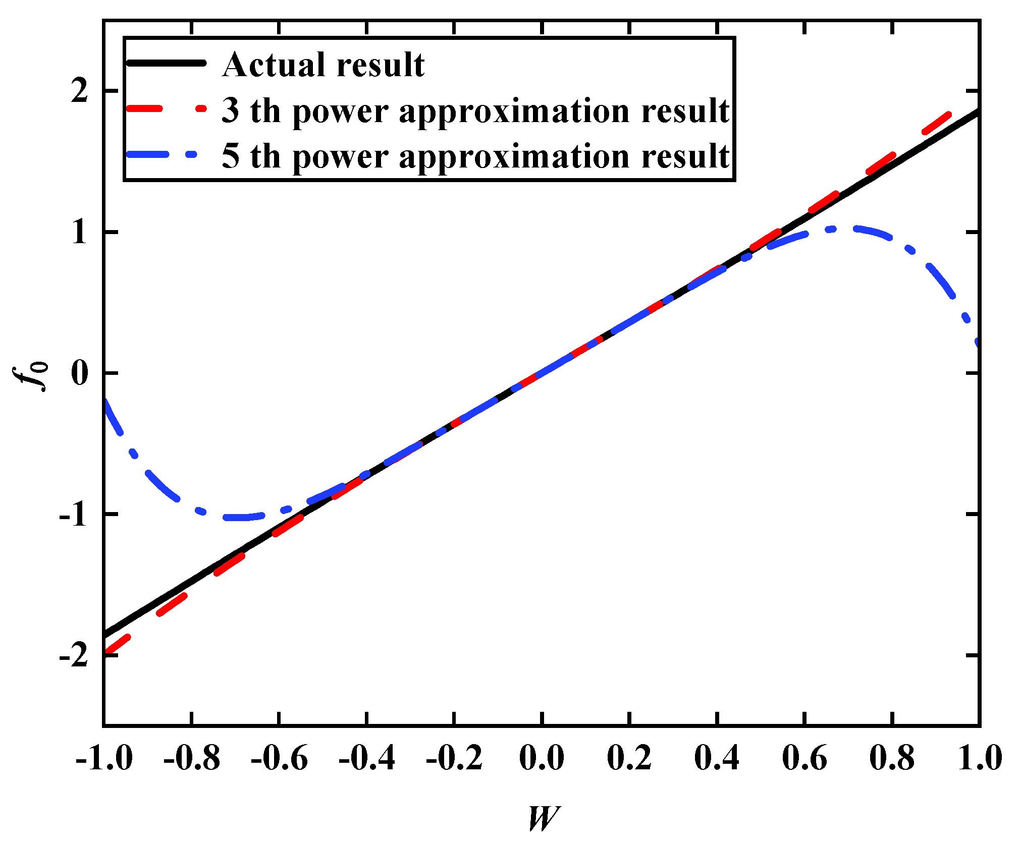
Substituting the dimensionless coefficients set above into Equations (1) and (2), the corresponding dimensionless forms of Equations (1) and (2) are obtained as follows:

$$f_0=2W\left(1-\frac{R}{\sqrt{W^2+1^2}}\right)$$

(3)

$$f_0\approx 2(W-RW+R{W}^3-9R{W}^5)$$

(4)

where W is the displacement produced by the motion of the tuned mass damper, f₀ is the restoring force, and R is the relative length of the spring. From Equations (3) and (4), a graph depicting the variation of the restoring force f₀ with the displacement W produced by the motion of the tuned mass damper can be plotted. As shown in Figure 2, the geometric nonlinearity generated by the linear spring leads to the generation of five times the stiffness nonlinearity, which can produce significant errors after moving away from the equilibrium position and has less research significance. Therefore, this paper used analyses based on the third power nonlinear stiffness.

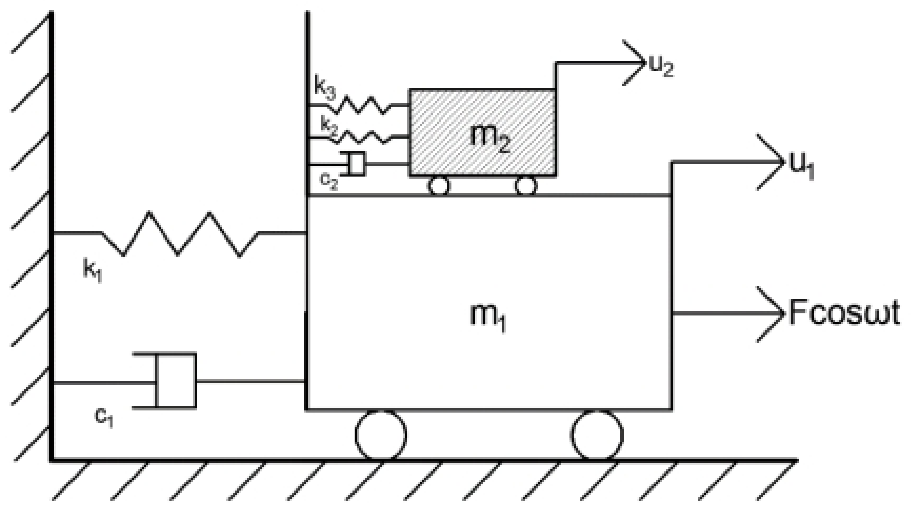
From the above analysis, the force–displacement relationship for the single-degree-of-freedom system considered in this paper is represented by $F_d=k_{2}x+k_3{x}^3$, $k_2>0$, and $k_3>0$, which correspond to the types of hardening considered in this paper. The mechanical model of the system is schematically shown in Figure 3, where the primary structure is subjected to harmonic excitation with an amplitude of $F$ and an excitation frequency of $\omega$.

The kinetic equation for a single degree of freedom system with a nonlinear TMD is derived from Newton’s second law as:

$$m_1{\ddot{u}}_1+c_1{\dot{u}}_1+k_1{u}_1+m_2{\ddot{u}}_2=F\cos \omega t$$

(5)

$$m_2{\ddot{u}}_2+c_2\left({\dot{u}}_2-{\dot{u}}_1\right)+k_2\left(u_2-u_1\right)+k_3{\left(u_2-u_1\right)}^3=0$$

(6)

where $m_1$, $c_1$, and $k_1$ represent the mass, damping, and linear spring stiffness of the primary structure; $m_2$, $c_2$, $k_2$, and $k_3$ represent the mass, damping, linear stiffness, and nonlinear stiffness of the TMD; $u_1$, $u_2$, and $u_2-u_1$ represent the displacement of the main structure, the displacement of the nonlinear TMD, and the relative displacement of the nonlinear TMD. The parameters $m_2$, $c_2$, and $k_2$ are the design variables in the design of TMD systems, and the parameter $k_3$ is the intrinsic coefficient required for the TMD to consider nonlinearity in practical applications. For the design variables in the TMD system, $c_2$ takes a fixed value, while $m_2$ and $k_2$ are the parameters to be determined.

By introducing dimensionless coefficients and using suitable variable substitutions, all units of parameters involving physical quantities are removed. This can clearly reflect the large parameters in the equation, making subsequent calculations easier. Furthermore, distinguishing the large and small parameters through the substitution of dimensionless coefficients can help identify the more important parameters in the design phase, making the calculation results of key parameters clear and unambiguous. First, the frequency of the controlled structure is $k_1/m_1={\omega }_1^2$, the frequency of the NTMD is $k_2/m_2={\omega }_2$, and the ratio of the mass of the NTMD to the mass of the controlled structure is called the mass ratio, set to $\epsilon {\alpha }_1$. To facilitate the study of the effect of the mass ratio parameter on the system, the product of the dimensionless minor parameter $\epsilon$ and the dimensionless parameter ${\alpha }_1$ was used in this paper to denote the mass ratio, which is $m_2/m_1=\epsilon {\alpha }_1$. The dimensionless minor parameter $\epsilon$ is a specific parameter, which is set to facilitate the use of subsequent approximate analytical methods. Next, the time variable is dimensionless; a new time variable $\tau ={\omega }_{1}t$ is used as the time variable of the equation, and the time variable $\tau$ is a dimensionless quantity. The selection of coordinates is crucial to the use of the subsequent analysis method. In this paper, we first used $x=u_1/L$ to denote the new coordinates and to carry out coordinate transformation and the dimensionless transformation of the original coordinates. Here we let $L$ be the unit length, whose role is only dimensionless, and $x$ can be regarded as the response of the main structure. Secondly, $y=(u_1-u_2)/L$ is used to denote another new coordinate, which is used to substitute the two coordinates of the original equation, and $y$ can be considered as the relative displacement of the controlled structure and the mass dampers. For the damping coefficient, since the damping ratio of the controlled structure is generally less than 5%, the original damping coefficient $c_1$ is replaced by the new dimensionless damping coefficient $\epsilon {\lambda }_1$, and the damping coefficient $c_2$ is replaced by the dimensionless damping coefficient ${\lambda }_2$. The dimensionless coefficient ${\alpha }_2$ represents the nonlinear stiffness, and $\omega$ is the excitation frequency. The ratio of NTMD frequency to controlled structure frequency is replaced by dimensionless quantity ${\mathsf{\Omega }}_2$, and the ratio of excitation frequency to controlled structure frequency is replaced by dimensionless quantity $\mathsf{\Omega }$. Meanwhile, the excitation force is expressed as a small quantity of the first order. The specific dimensionless coefficients are set as follows:

$$\begin{array}{l}\frac{F}{L{k}_1}=\epsilon f,\frac{m_2}{m_1}=\epsilon {\alpha }_1,\frac{u_1}{L}=x,\frac{u_1-u_2}{L}=y,\frac{k_1}{m_1}={\omega }_1^2,\frac{k_2}{m_2}={\omega }_2^2\\ {\omega }_{1}t=\tau ,\frac{\omega }{{\omega }_1}=\mathsf{\Omega },\frac{c_1}{m_1{\omega }_1}=\epsilon {\lambda }_1,\frac{c_2}{m_2{\omega }_1}={\lambda }_2,\frac{{\omega }_2}{{\omega }_1}={\mathsf{\Omega }}_2,\frac{k_3{L}^2}{k_2}={\alpha }_2\end{array}$$

Substituting the above dimensionless coefficients into Equations (5) and (6), the equation of motion can be written as:

$$\ddot{x}+x+\epsilon \left({\alpha }_1{\lambda }_2\dot{y}+{\alpha }_1{\mathsf{\Omega }}_2^{2}y+{\alpha }_1{\alpha }_2{\mathsf{\Omega }}_2^2{y}^3+{\lambda }_1\dot{x}\right)=\epsilon f\cos \mathsf{\Omega }\tau$$

(7)

$$\frac{\ddot{y}}{1+\epsilon {\alpha }_1}+\frac{\epsilon {\lambda }_1\dot{x}}{1+\epsilon {\alpha }_1}+\frac{x}{1+\epsilon {\alpha }_1}+{\lambda }_2\dot{y}+{\mathsf{\Omega }}_2^{2}y+{\alpha }_2{\mathsf{\Omega }}_2^2{y}^3=\frac{\epsilon f\cos \mathsf{\Omega }\tau }{1+\epsilon {\alpha }_1}$$

(8)

3. Approximate Analytical Solution of the Equations of Motion of the System

To facilitate the use and calculation of subsequent analytical methods, Equations (7) and (8) are decoupled through Taylor’s formula. Equations (7) and (8) are considered to be functions of the mass ratio $\epsilon$ and are expanded by Taylor’s formula near $\epsilon =0$. Only the primary term is retained because $\epsilon$ itself is small, and the first order expansion is sufficient for subsequent analysis. The above expressions can be written as follows:

$$r\left(\epsilon \right)=r\left(0\right)+\epsilon r^{\prime }\left(0\right)$$

(9)

Substituting Equation (9) into Equations (7) and (8), the following new equation can be obtained:

$$\ddot{x}+x+\epsilon \left({\alpha }_1{\lambda }_2\dot{y}+{\alpha }_1{\mathsf{\Omega }}_2^{2}y+{\alpha }_1{\alpha }_2{\mathsf{\Omega }}_2^2{y}^3+{\lambda }_1\dot{x}-f\cos \mathsf{\Omega }\tau \right)=0$$

(10)

$$\ddot{y}+y+\epsilon \delta \left({\mathsf{\Omega }}_2^{2}y+{\alpha }_2{\mathsf{\Omega }}_2^2{y}^3+{\lambda }_2\dot{y}+x-y\right)=0$$

(11)

Among them: $\epsilon \delta =1$.

Higher-order terms are eliminated from Equations (10) and (11) because they are less significant in the current study, and only the necessary parameter terms are retained. The complex variable averaging method can simplify the process of operation by assuming the steady-state response of the nonlinear TMD as a first-order harmonic approximation with the same equivalent excitation frequency. By setting the solution of the equation in the following form and substituting the set solution into Equations (10) and (11), the second-order system of equations can be reduced to a first-order system for subsequent analysis.

The complex variable averaging method is mainly in the form of complexification, i.e., replacing the displacement and velocity variables of the system with complex variables. Therefore, it can reduce the original system equations from second order to first order. This approach simplifies the representation based on expansion methods, such as Fourier series expansion or Taylor expansion. The problem studied in this paper is related to the phenomena arising from the 1:1 resonance of the system. The calculation based on the averaging method of complex variables can focus on the 1:1 resonance frequency of the system and facilitate the relationship between the nonlinear coefficients of the system and the vibration reduction effect of the tuned mass dampers. The averaging method takes the amplitude and phase of the solution as time-dependent parameters and averages the derivatives corresponding to the amplitude and phase of the system. The complex variable-averaging method also follows this approach, but it sets the solution in the form of a complex number, which is more conducive to the solution process. The complex variable-averaging method assumes the vibration as a harmonic wave in complex form with the same frequency as the external excitation. This assumption is similar to the derivation of the averaging method, and the first-order approximate solutions of Equations (10) and (11) can be set as follows:

$$x=\frac{1}{2i\mathsf{\Omega }}{A}_1{e}^{i\mathsf{\Omega }t}+cc$$

(12)

$$y=\frac{1}{2i\mathsf{\Omega }}{A}_2{e}^{i\mathsf{\Omega }t}+cc$$

(13)

where $A_1$ is the complex variable, consisting of the steady-state amplitude and phase of the main structure; $A_2$ is the complex variable, consisting of the steady-state amplitude and phase of the nonlinear TMD; $\mathsf{\Omega }$ is the ratio of the excitation frequency to the frequency of the controlled structure; and $cc$ substitutes the conjugate complex in the first half of the equation.

Correspondingly, the two sides of Equations (12) and (13) give expressions for $\dot{x}$ and $\dot{y}$ by means of derivatives for time $t$. The same is true for $\ddot{x}$ and $\ddot{y}$. Deriving the two sides of the equations for $\dot{x}$ and $\dot{y}$, we obtained:

$$\dot{x}=\frac{1}{2}{A}_1{e}^{i\mathsf{\Omega }t}+cc$$

(14)

$$\dot{y}=\frac{1}{2}{A}_2{e}^{i\mathsf{\Omega }t}+cc$$

(15)

$$\ddot{x}={\dot{A}}_1{e}^{i\mathsf{\Omega }t}+\frac{1}{2}i\mathsf{\Omega }{A}_1{e}^{i\mathsf{\Omega }t}+cc$$

(16)

$$\ddot{y}={\dot{A}}_2{e}^{i\mathsf{\Omega }t}+\frac{1}{2}i\mathsf{\Omega }{A}_2{e}^{i\mathsf{\Omega }t}+cc$$

(17)

The results of the complex variable averaging method are more concise compared to the averaging method. That is, its complex form is somewhat shorter than the trigonometric form, and its analysis is simpler to perform. By substituting Equations (12)–(17) into Equations (10) and (11), two coupled systems of first-order differential equations can be obtained. Since this paper is only concerned with the case near the 1:1 resonance, let $\omega ={\omega }_1=1$. The $e^{i\omega t}$ term is retained first. This term can be viewed as a rapidly varying simple harmonic vibration approximation term with a frequency of 1, and then the term is removed after averaging according to the previous principle. Equations (10) and (11) can be rewritten after finishing as:

$$\begin{array}{l}2{\dot{A}}_1+i\mathsf{\Omega }{A}_1+\frac{1}{i\mathsf{\Omega }}{A}_1+\\ \hspace{1em}\hspace{1em}\epsilon \left({\alpha }_1{\lambda }_2{A}_2+\frac{1}{i\mathsf{\Omega }}{\alpha }_1{\mathsf{\Omega }}_2^2{A}_2-\frac{3}{4{\mathsf{\Omega }}^3}i{\alpha }_1{\alpha }_2{\mathsf{\Omega }}_2^2{\left|A_2\right|}^2{A}_2+{\lambda }_1{A}_1-f\right)=0\end{array}$$

(18)

$$\begin{array}{l}2{\dot{A}}_2+i\mathsf{\Omega }{A}_2+\frac{1}{i\mathsf{\Omega }}{A}_2+\\ \hspace{1em}\hspace{1em}\epsilon \delta \left(-\frac{1}{\mathsf{\Omega }}i{\mathsf{\Omega }}_2^2{A}_2-\frac{3}{4{\mathsf{\Omega }}^3}i{\alpha }_2{\mathsf{\Omega }}_2^2{\left|A_2\right|}^2{A}_2+{\lambda }_2{A}_2-\frac{1}{\mathsf{\Omega }}i{A}_1+\frac{1}{\mathsf{\Omega }}i{A}_2\right)=0\end{array}$$

(19)

Other scholars have shown [27,28] that the maximum first-order structural response is obtained when the excitation frequenc30y is near the first-order structural frequency. Since only the case near the 1:1 resonance is of interest, the excitation frequency can be considered equal to the first-order structural frequency; thus, $\mathsf{\Omega }=1$. Substituting this into Equations (18) and (19), it was found that:

$$2{\dot{A}}_1+\epsilon \left({\alpha }_1{\lambda }_2{A}_2-i{\alpha }_1{\mathsf{\Omega }}_2^2{A}_2-\frac{3}{4}i{\alpha }_1{\alpha }_2{\mathsf{\Omega }}_2^2{\left|A_2\right|}^2{A}_2+{\lambda }_1{A}_1-f\right)=0$$

(20)

$$2{\dot{A}}_2+\epsilon \delta \left(-i{\mathsf{\Omega }}_2^2{A}_2-\frac{3}{4}i{\alpha }_2{\mathsf{\Omega }}_2^2{\left|A_2\right|}^2{A}_2+{\lambda }_2{A}_2-i{A}_1+i{A}_2\right)=0$$

(21)

Many studies have concluded [29,30] that the amplitude does not vary with time when the structure is at a steady-state amplitude. This is true for both the amplitude of the primary structure and the amplitude of the tuned mass dampers. In this paper, we studied the steady-state response; thus, the first-order derivatives in Equations (20) and (21) are zero. This gives the following:

$${\alpha }_1{\lambda }_2{A}_2-i{\alpha }_1{\mathsf{\Omega }}_2^2{A}_2-\frac{3}{4}i{\alpha }_1{\alpha }_2{\mathsf{\Omega }}_2^2{\left|A_2\right|}^2{A}_2+{\lambda }_1{A}_1-f=0$$

(22)

$$-i{\mathsf{\Omega }}_2^2{A}_2-\frac{3}{4}i{\alpha }_2{\mathsf{\Omega }}_2^2{\left|A_2\right|}^2{A}_2+{\lambda }_2{A}_2-i{A}_1+i{A}_2=0$$

(23)

Equations (22) and (23) can be decoupled by adding and subtracting from each other in a simplified way, and then the decoupled equations can be organized to obtain:

$${\alpha }_1{\lambda }_2{A}_2-i{\alpha }_1{\mathsf{\Omega }}_2^2{A}_2-\frac{3}{4}i{\alpha }_1{\alpha }_2{\mathsf{\Omega }}_2^2{\left|A_2\right|}^2{A}_2+{\lambda }_1{A}_1-f=0$$

(24)

$$A_1=-{\mathsf{\Omega }}_2^2{A}_2-\frac{3}{4}{\alpha }_2{\mathsf{\Omega }}_2^2{\left|A_2\right|}^2{A}_2-i{\lambda }_2{A}_2+A_2$$

(25)

Substituting Equation (25) into Equation (24), we can obtain the equation related to $A_2$ only, as follows:

$$\begin{array}{l}{\alpha }_1{\lambda }_2{A}_2-i{\alpha }_1{\mathsf{\Omega }}_2^2{A}_2-\\ \hspace{1em}\frac{3}{4}i{\alpha }_1{\alpha }_2{\mathsf{\Omega }}_2^2{\left|A_2\right|}^2{A}_2-{\lambda }_1{\mathsf{\Omega }}_2^2{A}_2-\frac{3}{4}{\alpha }_2{\lambda }_1{\mathsf{\Omega }}_2^2{\left|A_2\right|}^2{A}_2-i{\lambda }_1{\lambda }_2{A}_2+{\lambda }_1{A}_2-f=0\end{array}$$

(26)

By expanding $A_2$ in Equation (26) into the form of complex numbers, substituting the expansion into Equation (26), and then separating the real and imaginary parts, we could obtain nonlinear Equations (27) and (28) with respect to amplitude and phase as follows:

$${\alpha }_1{\lambda }_2{a}_2-{\lambda }_1{\mathsf{\Omega }}_2^2{a}_2-\frac{3}{4}{\lambda }_1{\alpha }_2{\mathsf{\Omega }}_2^2{a}_2^3+{\lambda }_1{a}_2=f\cos b$$

(27)

$${\alpha }_1{\mathsf{\Omega }}_2^2{a}_2+\frac{3}{4}{\alpha }_1{\alpha }_2{\mathsf{\Omega }}_2^2{a}_2^3+{\lambda }_1{\lambda }_2{a}_2=f\sin b$$

(28)

By adding Equations (27) and (28) squared, the redundant trigonometric functions can be eliminated to obtain a sixfold equation related only to the tuned mass damper amplitude $a_2$. After organizing the equations, we can obtain:

$$\begin{array}{l}\left\{{\left[\frac{\left(3{\alpha }_1{\alpha }_2{a}_2^3\right)}{4}+{\alpha }_1{a}_2\right]}^2+{\left[\frac{\left(3{\lambda }_1{\alpha }_2{a}_2^3\right)}{4}+{\lambda }_1{a}_2\right]}^2\right\}{\mathsf{\Omega }}_2^4+\\ \left\{\left(2{\lambda }_1{\lambda }_2{a}_2\right)\left[\frac{\left(3{\alpha }_1{\alpha }_2{a}_2^3\right)}{4}+{\alpha }_1{a}_2\right]-2\left({\lambda }_1{a}_2+{\lambda }_2{\alpha }_1{a}_2\right)\left[\frac{\left(3{\lambda }_1{\alpha }_2{a}_2^3\right)}{4}+{\lambda }_1{a}_2\right]\right\}{\mathsf{\Omega }}_2^2\\ +{\left({\lambda }_{1}a+{\lambda }_2{\alpha }_1{a}_2\right)}^2+{\lambda }_1^2{\lambda }_2^2{a}_2^2-f^2=0\end{array}$$

(29)

Equation (29) has a more complex and confusing form, which does not facilitate subsequent calculations and analysis. Equation (29) can be rectified and transformed into an equation about $z$, where $z=a_2^2$:

$$\begin{array}{l}\left[\left(\frac{9{\alpha }_1^2{\alpha }_2^2{\mathsf{\Omega }}_2^4}{16}\right)+\left(\frac{9{\lambda }_1^2{\alpha }_2^2{\mathsf{\Omega }}_2^4}{16}\right)\right]z^3+\\ \left\{\frac{\left[3{\alpha }_1{\alpha }_2{\mathsf{\Omega }}_2^2\left({\alpha }_1{\mathsf{\Omega }}_2^2+{\lambda }_1{\lambda }_2\right)\right]}{2}-\frac{\left[3{\lambda }_1{\alpha }_2{\mathsf{\Omega }}_2^2\left(-{\lambda }_1{\mathsf{\Omega }}_2^2+{\lambda }_1+{\lambda }_2{\alpha }_1\right)\right]}{2}\right\}{z}^2\\ +\left[{\left({\alpha }_1{\mathsf{\Omega }}_2^2+{\lambda }_1{\lambda }_2\right)}^2+{\left(-{\lambda }_1{\mathsf{\Omega }}_2^2+{\lambda }_1+{\lambda }_2{\alpha }_1\right)}^2\right]z-f^2=0\end{array}$$

(30)

In Equation (30), all the variables except $z$ are already known; thus, the value of $z$ can be found.

The approximate analytical solution of the structural frequency response was obtained up to this point, and it is unknown whether the final derived modulation demodulation equation is correct. The correctness and accuracy of the equation need to be further determined by comparison and verification.

4. System Optimal Parameter Design

The modulation and demodulation equations of the system were obtained in the previous section by deriving the equations of motion through the complex variable averaging method. In the traditional TMD design method, it is generally considered that the TMD is linear, and the linear TMD designed according to the optimal linearity absorbs the energy of structural vibration so that the steady-state amplitude of the primary structure is as small as possible at different excitation frequencies to maintain the stability of the primary structure to the maximum extent. In the frequency response curve, a better control effect can be achieved when the left and right peak amplitudes of the primary structure are equal. However, if the nonlinearity of the TMD is considered under the conditions of practical engineering applications, the TMD cannot achieve the best control effect if it is designed according to the traditional linear design method. Therefore, it is necessary to consider the nonlinear characteristics of the TMD in order to achieve a better control performance of the structure.

In order to verify the correctness and accuracy of the approximate analytical solutions obtained in the previous section, Equations (7), (8), and (30) were computed separately. In this paper, the linear primary structure connected with the TMD was selected as the object of study, and the relevant parameters of the primary structure were set as follows:

$$m_1=1 \mathrm{k}\mathrm{g},k_1=1 \mathrm{N}\mathrm{/}\mathrm{m},c_1=0.1 \mathrm{N}\mathrm{\cdot }\mathrm{s}\mathrm{/}\mathrm{m}$$

The mass ratio of the TMD to the primary structure was tentatively set at 0.02, and the remaining design parameters were determined based on the optimized equation for linear TMD design with damping:

$$m_2=0.02 \mathrm{k}\mathrm{g},c_2=0.0031 \mathrm{N}\mathrm{\cdot }\mathrm{s}\mathrm{/}\mathrm{m},k_2=0.0161 \mathrm{N}\mathrm{/}\mathrm{m}$$

The corresponding dimensionless parameters could also be obtained as:

$${\lambda }_1=5,{\lambda }_2=0.155,f=15$$

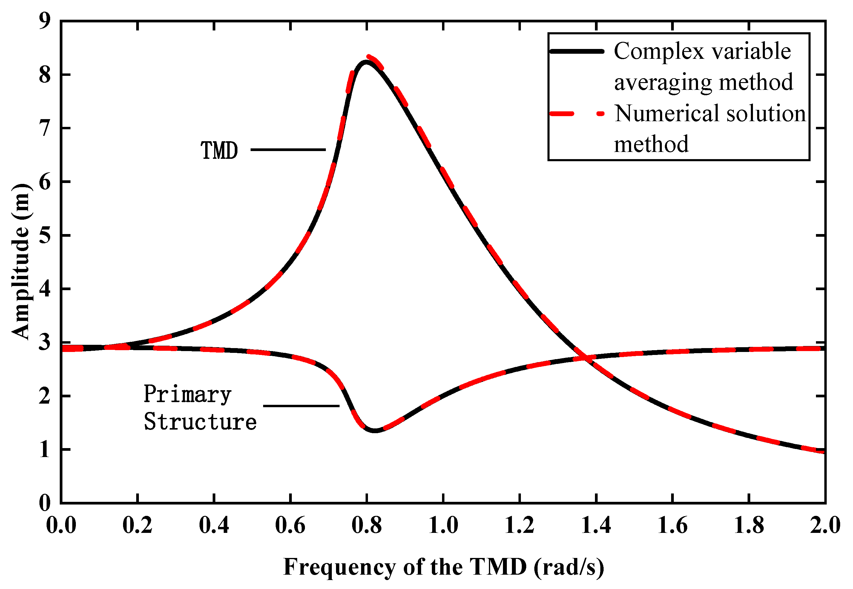
This resulted in a frequency–amplitude curve related to the TMD frequency. Figure 4 shows the frequency–amplitude curves of the structure, where the horizontal coordinate is the intrinsic frequency of the TMD and the vertical coordinate is the amplitude. The solid black line is the result obtained by the complex variable averaging method, and the red dashed line is the result obtained by the numerical method. The graph shows that the curves obtained by the complex variable averaging method and the numerical method are close to each other with almost no error. It can be seen that the modulation demodulation equation obtained by the complex variable averaging method is highly accurate and meets the accuracy requirement.

Table 1. Optimal frequency of the tuned mass dampers.

${\mathit{\alpha }}_1$	${\mathit{\alpha }}_2$	Numerical Solution Method (rad/s)	Complex Variable Averaging Method (rad/s)
1	0.01	0.817	0.821
	0.02	0.708	0.711
2	0.01	0.916	0.918
	0.02	0.846	0.848
3	0.01	0.958	0.957
	0.02	0.914	0.912
4	0.01	0.978	0.976
	0.02	0.947	0.946
5	0.01	0.987	0.987
	0.02	0.965	0.965

shows ten combinations (columns 1 and 2 of the table) where the structural mass ratios ${\alpha }_1$ are 1, 2, 3, 4, and 5, and the nonlinear stiffnesses ${\alpha }_2$ are 0.01 and 0.02. Other parameters were held constant. For various combinations of ${\alpha }_1$ and ${\alpha }_2$, the approximate analytical solution of the optimal design frequency was obtained using Equation (30) to compare with the solution obtained by the conventional numerical method. From the data in Table 1, it was concluded that the average error between the approximate analytical solution and the numerical method was 0.0017, and the average error rate was 0.188%. Although there were some errors between the results of the complex variable averaging method and the traditional numerical method, the errors were very small and even negligible. The accuracy of Equation (30) was proven to be very high; thus, the correctness of the modulation demodulation equation obtained by the complex variable averaging method is known, and the equation can be used for subsequent analysis.

Inherent frequency is a key parameter in TMD design. Choosing a suitable frequency enables the TMD to achieve better control performance, and the corresponding response amplitude of the primary structure will be relatively small. In the frequency–amplitude curve, the frequency ${\omega }_2$ corresponding to the maximum amplitude point generated by the TMD and the minimum amplitude point generated by the primary structure represent the theoretical optimum design value of TMD frequency. Figure 4 shows the frequency–amplitude curves of the primary structure and the TMD obtained by numerical and complex variable averaging methods of the system equations of motion, from which it was concluded that when ${\omega }_2$ = 0.821, the corresponding TMD amplitude is maximum, and the amplitude of the primary structure is minimum. That is, the theoretical optimum design value of the TMD frequency of the system can be considered 0.821.

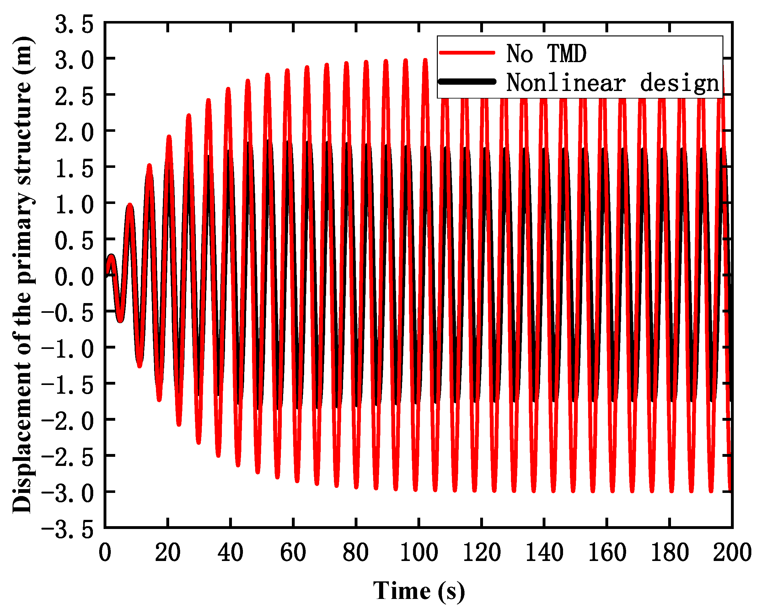
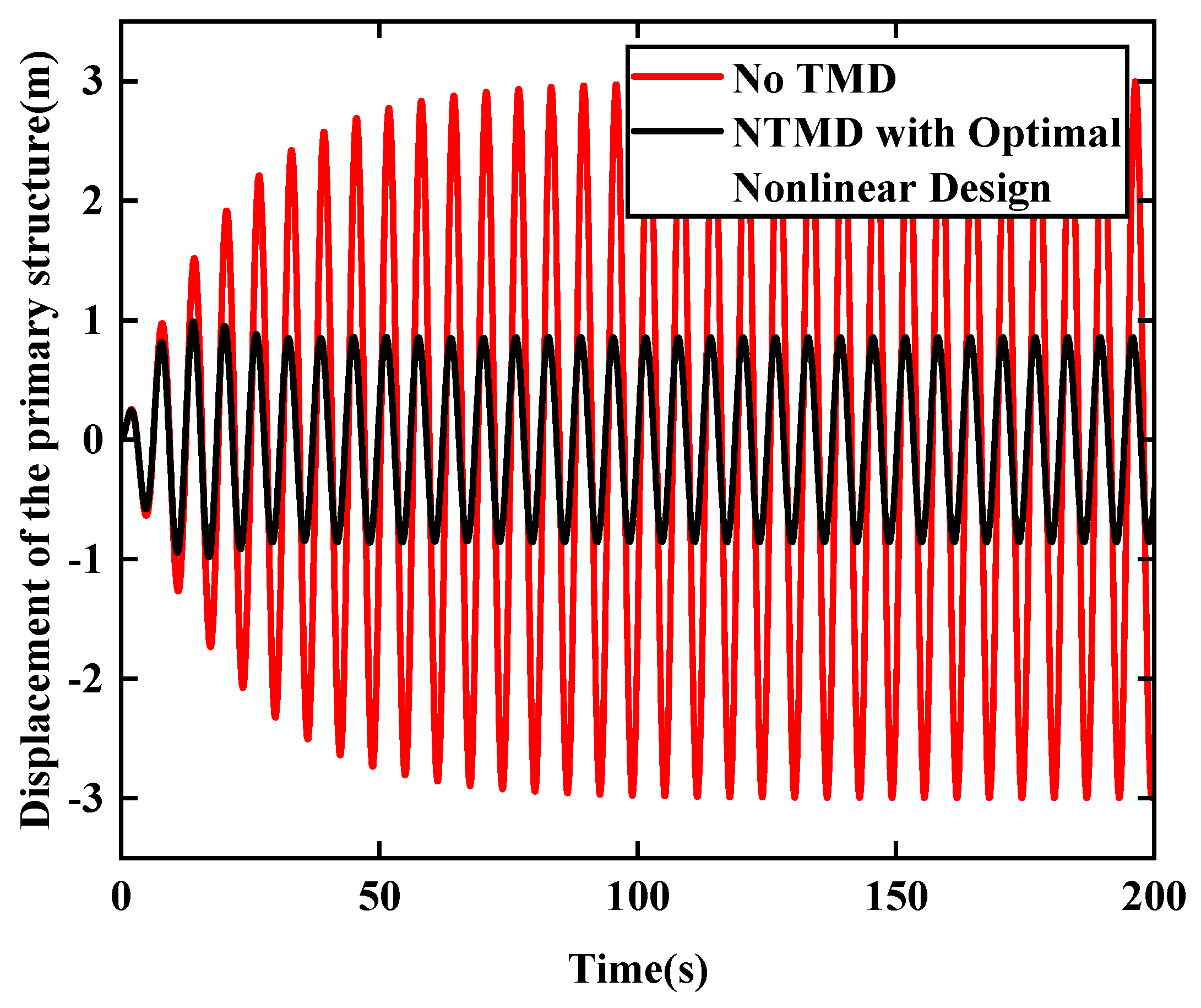
Figure 5 shows the comparison of the steady-state displacement time diagrams obtained for the primary structure without TMD and the primary structure under nonlinear TMD control when ${\omega }_2$ = 0.821 and other parameters are constant. As can be seen in Figure 5, the steady-state displacement of the primary structure with the non-linear TMD installed at this frequency was significantly smaller than the steady-state displacement of the primary structure without the TMD. The steady-state displacement was reduced by about 35.90%, which fully proves the effectiveness of the nonlinear TMD control effect at this frequency. 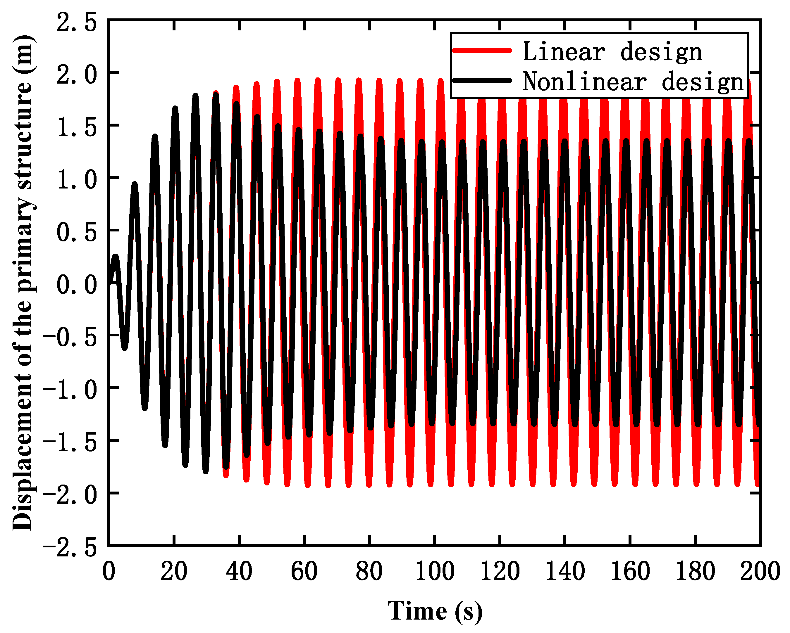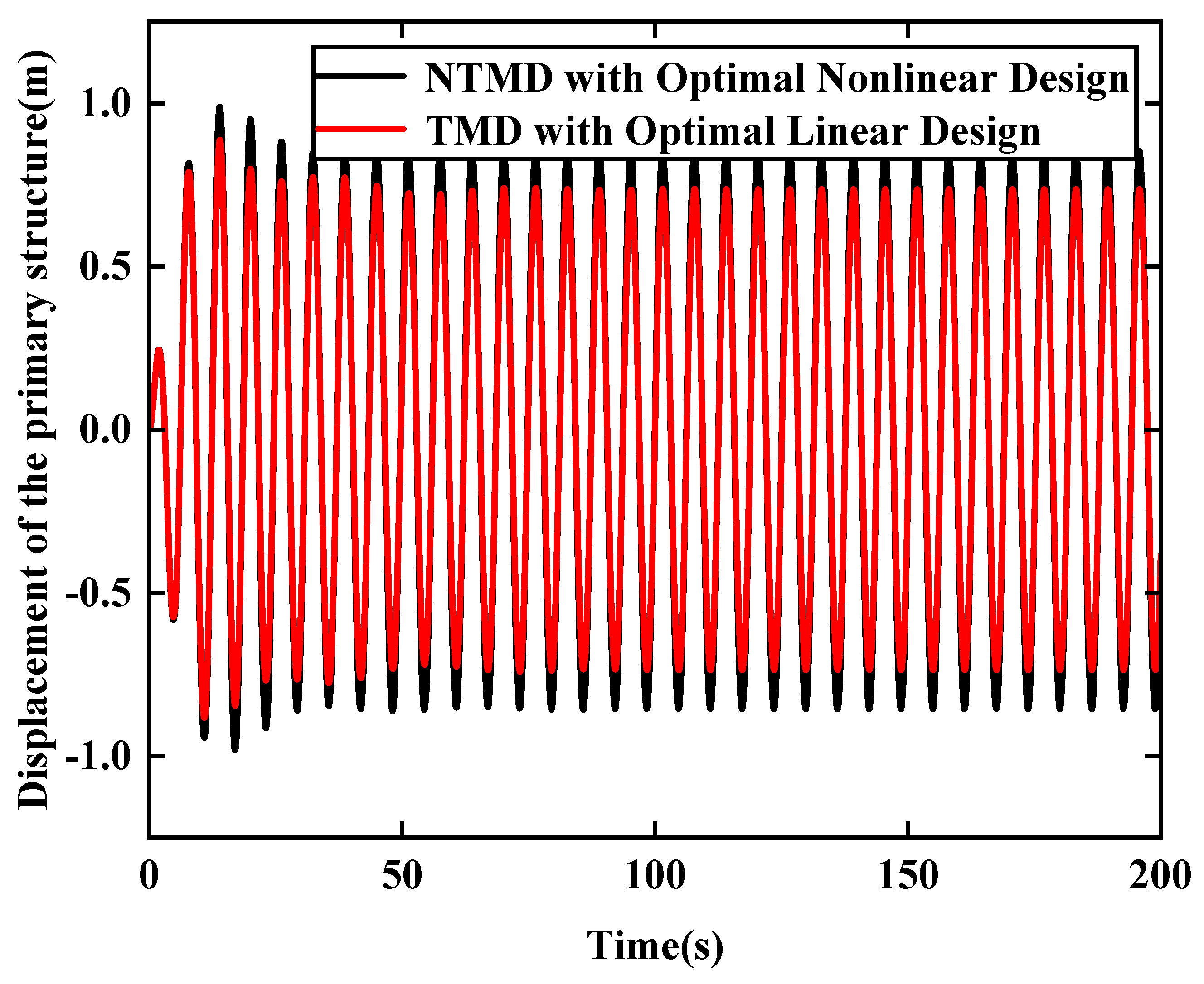Figure 6 shows the comparison of the steady-state displacement time plots of the first-stage structure under the control of the ideal linear TMD and the optimized nonlinear TMD. From Figure 6, it can be seen that the steady-state displacement of the first-stage structure with the nonlinear TMD installed at this frequency was smaller than the steady-state displacement of the first-stage structure with the optimal linear TMD. The transient response of the primary structure was partially the same, and the steady-state displacement was reduced by about 9.05%. The ideal linear TMD is a hypothetical linear TMD without any nonlinear characteristics generated during the vibration, which cannot exist in reality. It can be seen that when the design frequency ${\omega }_2$ = 0.821, the nonlinear TMD achieved good control effectiveness, and subsequent steady-state analysis was performed based on this design frequency.

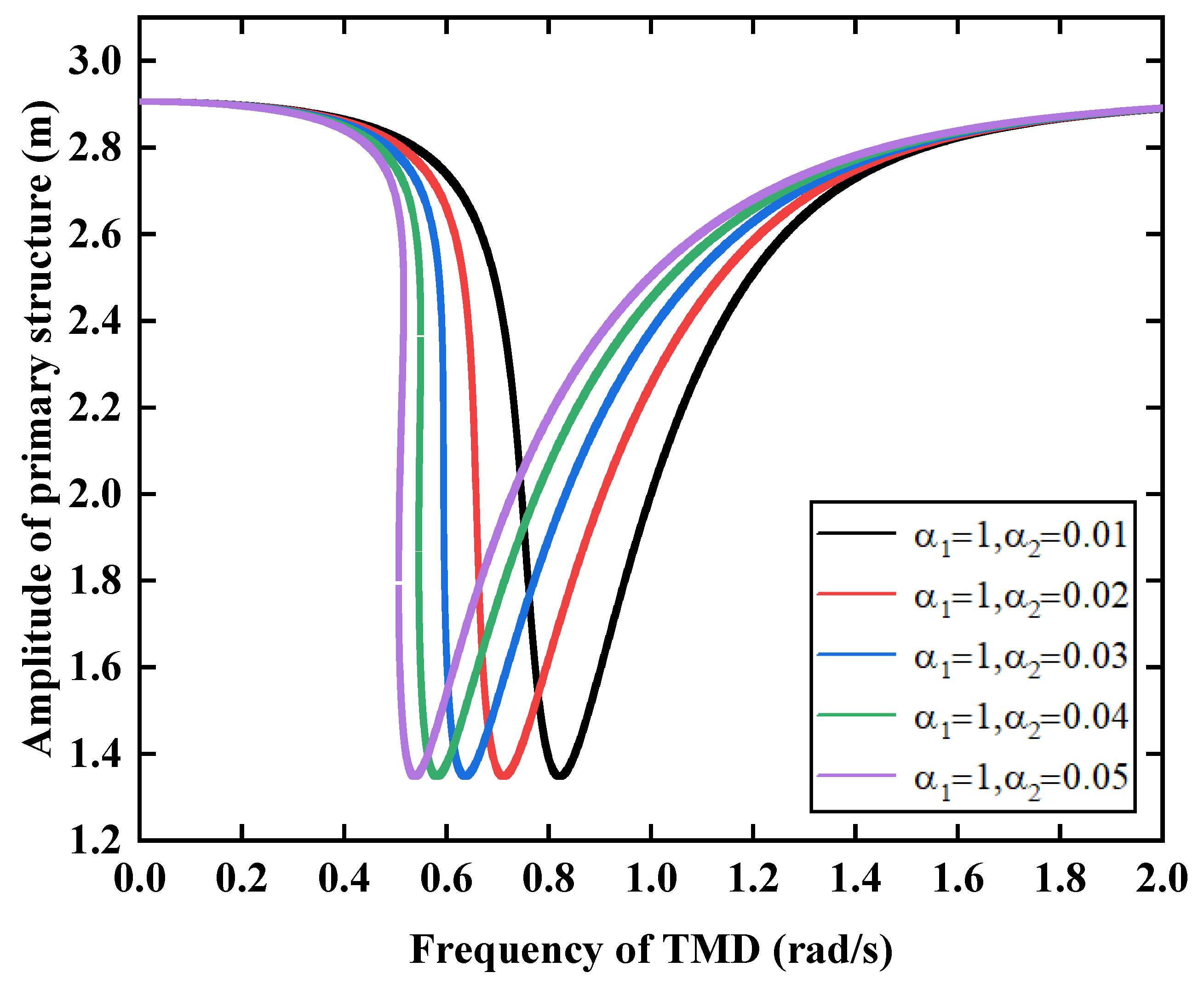
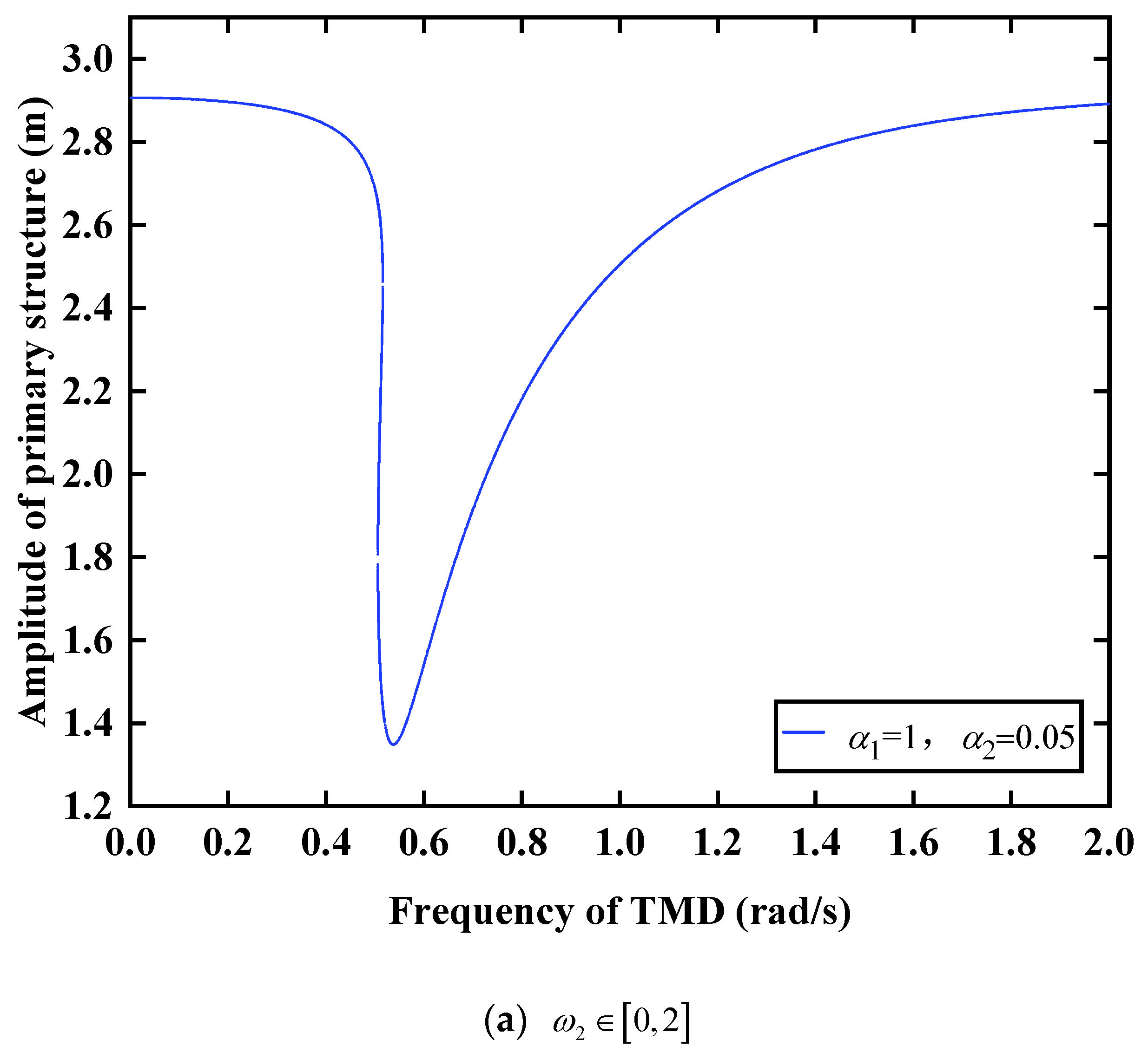
In order to study the effect of increasing nonlinear coefficients on the amplitude of the structure, frequency–amplitude curves corresponding to different nonlinear coefficients were obtained by taking ${\alpha }_2$ values of 0.01, 0.02, 0.03, 0.04, and 0.05, as shown in Figure 7. Observing Figure 7, the horizontal coordinate represents the intrinsic frequency of the TMD, and the vertical coordinate represents the displacement amplitude of the primary structure. With the increase in the nonlinearity coefficient, the frequency–amplitude curve of the primary structure gradually shifted to the left, and the optimal frequency for structure control changed. 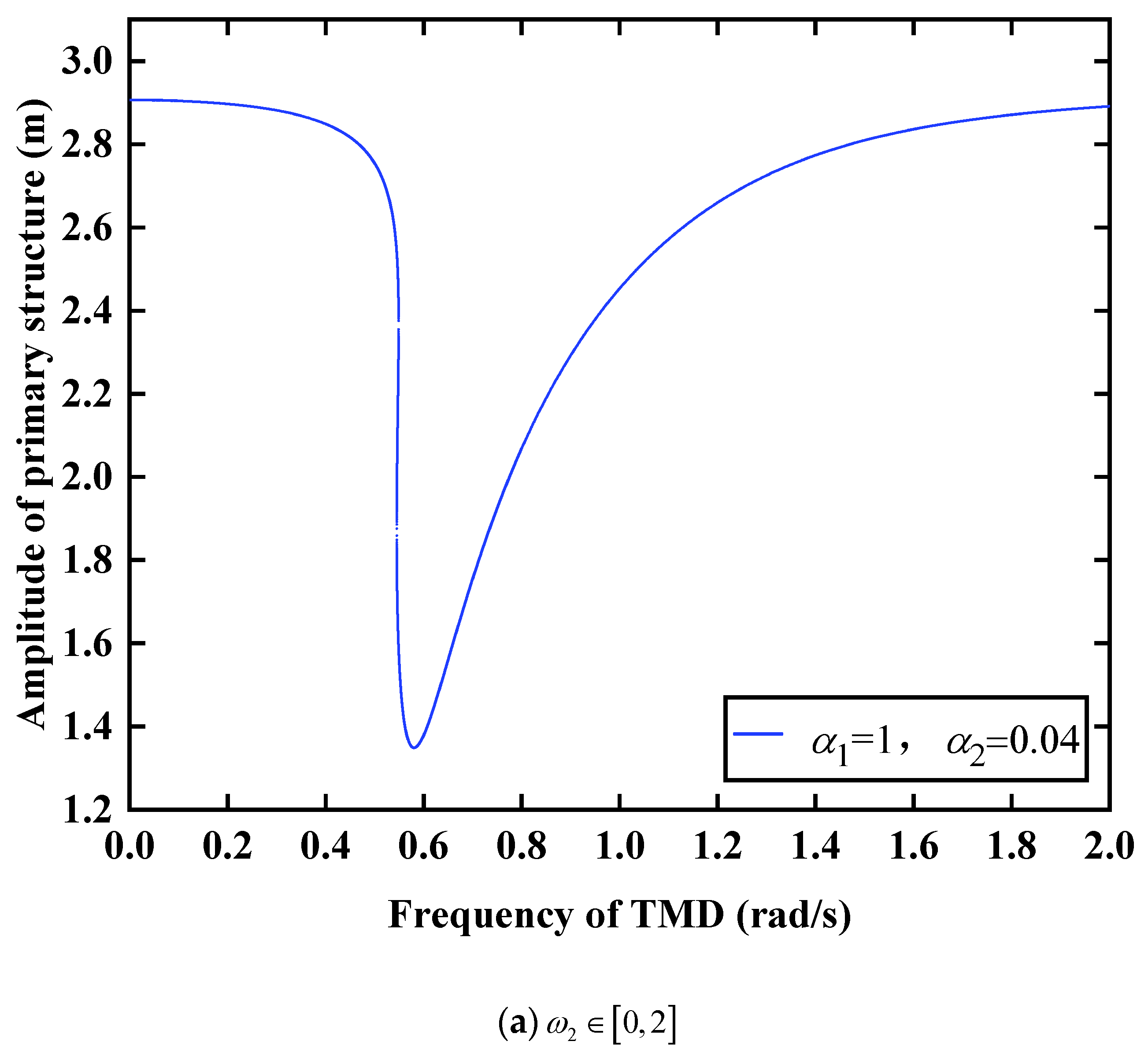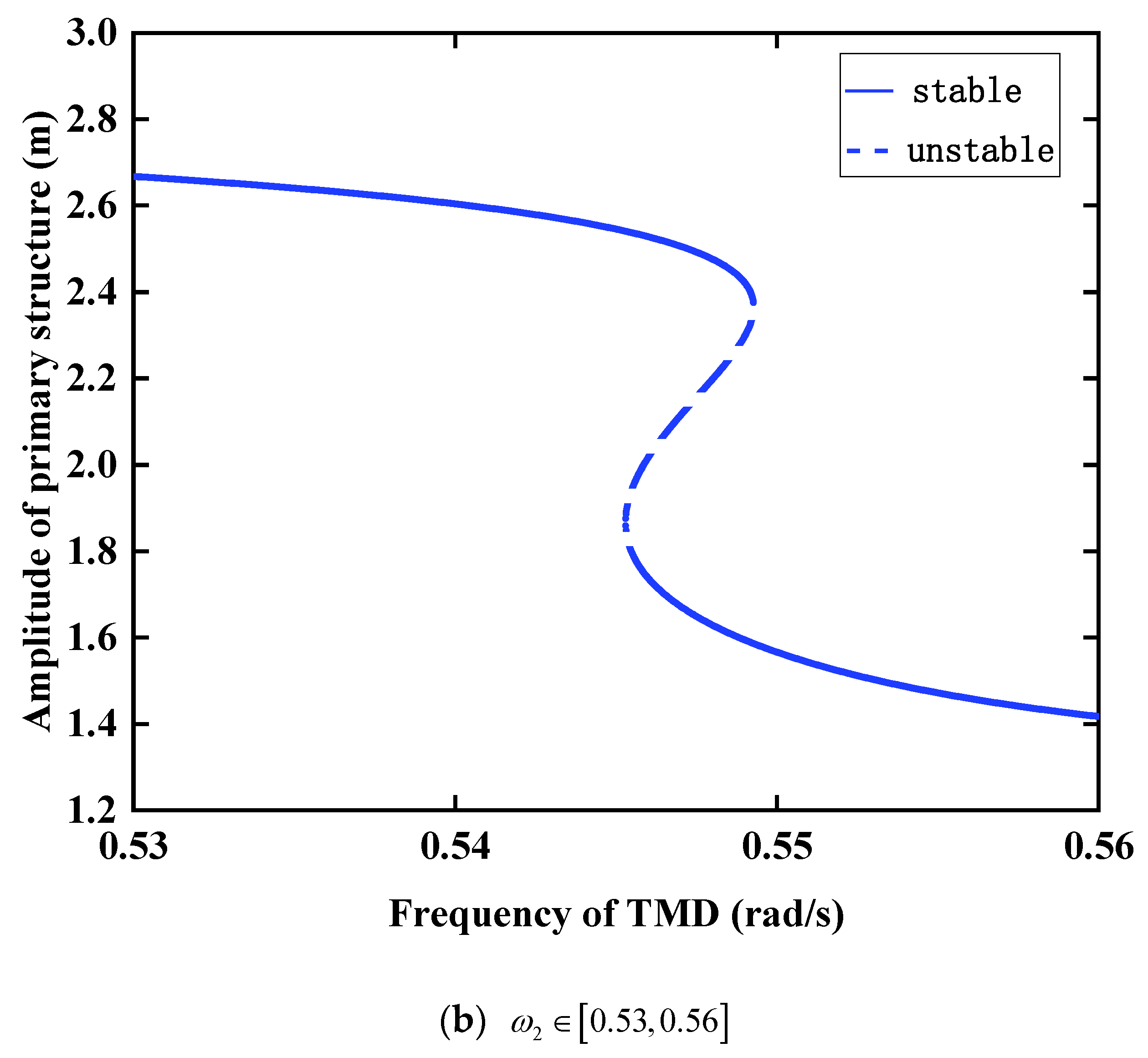As shown in Figure 8a, when ${\alpha }_2$ increased to 0.04, the frequency–amplitude curve exhibited a multi-valued phenomenon in the interval of TMD frequency ${\omega }_2$ values of 0.545–0.550. For the convenience of observation, the interval where the multi-valued phenomenon occurred was enlarged. As shown in Figure 8b, the dashed part of the blue curve corresponds to multiple amplitude values at the same TMD frequency. 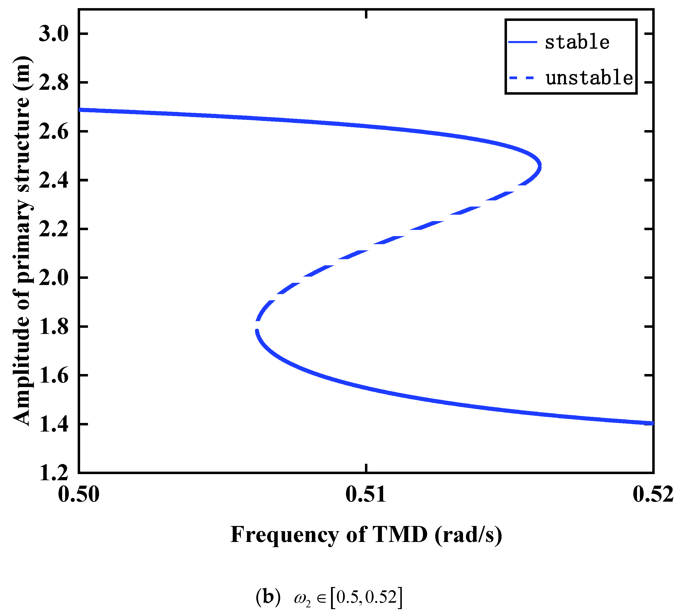Similarly, Figure 9a shows the frequency–amplitude curve of the structure at ${\alpha }_2=$ 0.05. From Figure 9b, the range of TMD frequencies ${\omega }_2$ where the multi-valued phenomenon appeared was 0.505–0.515, which was expanded (compared to the range of TMD frequencies where the multi-valued phenomenon appeared at ${\alpha }_2=$ 0.04). When multiple values appear in the frequency–amplitude plot, it indicates that the structure is in an unstable state in this frequency interval, and jumps may occur, which may have adverse effects on the structure. It is possible that two or more structural amplitude values may occur at the same frequency, resulting in static bifurcation. As the nonlinear coefficient increased, the minimum amplitude value of the structure did not change; thus, increasing the nonlinear coefficient does not improve the control performance of the TMD on the structure. The nonlinear coefficient is not required to be as small as possible, and the impact of considering the nonlinearity on the control performance of the TMD could not be obviously observed during the study. Thus, the most suitable value for the nonlinear coefficient was determined to be ${\alpha }_2=$ 0.02.

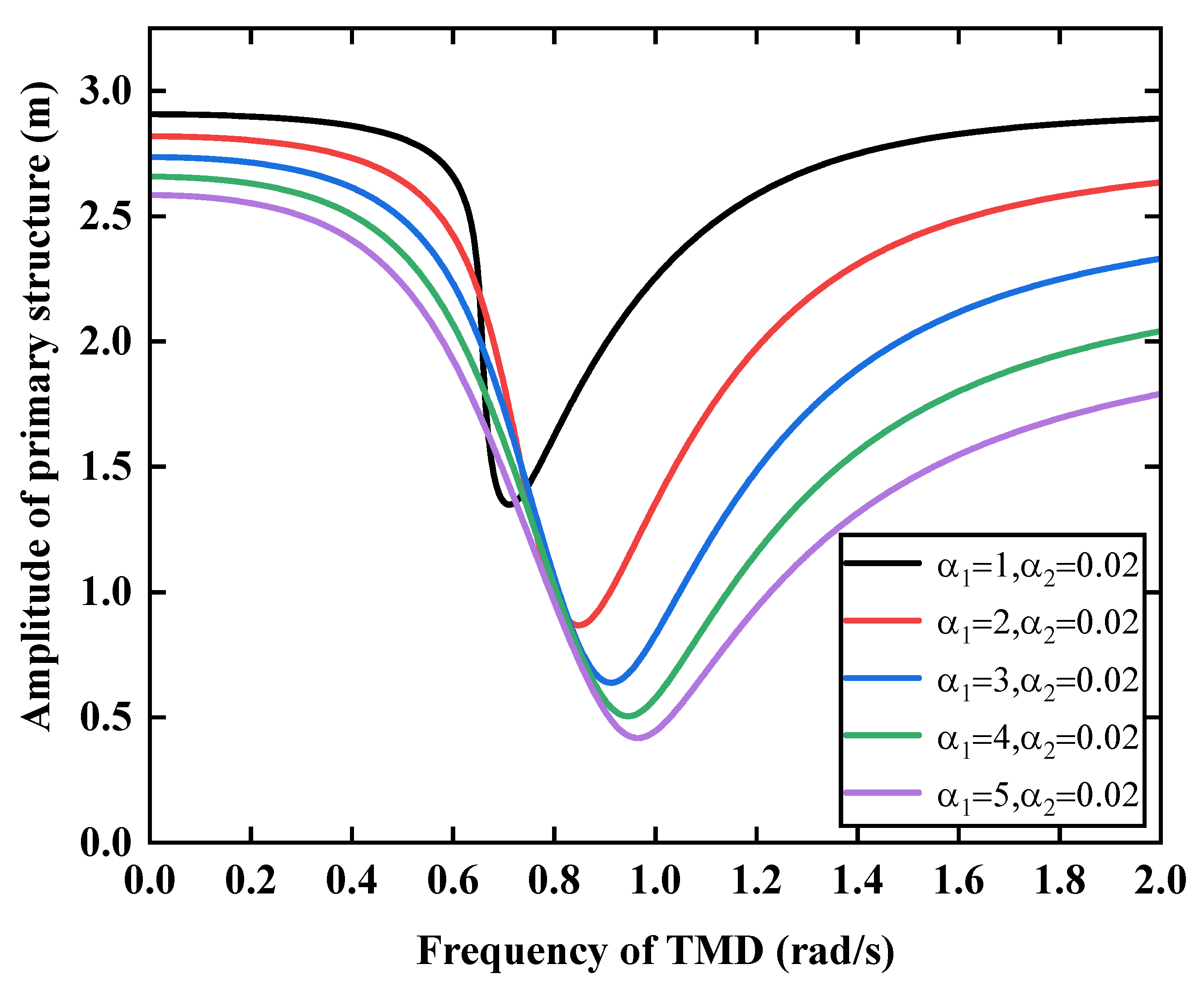
Figure 10 shows the frequency–amplitude curves of the NTMD compared to those of the primary structure for mass ratios ${\alpha }_1=$ 1, 2, 3, 4, and 5. It can be seen from Figure 10 that the maximum amplitude of the primary structure gradually decreased with an increasing mass ratio, and the frequency–amplitude curve of the structure gradually shifted to the right. The best control effect of NTMD was achieved when the mass ratio ${\alpha }_1=$ 5, i.e., the mass of NTMD was 10% of the mass of the primary structure. 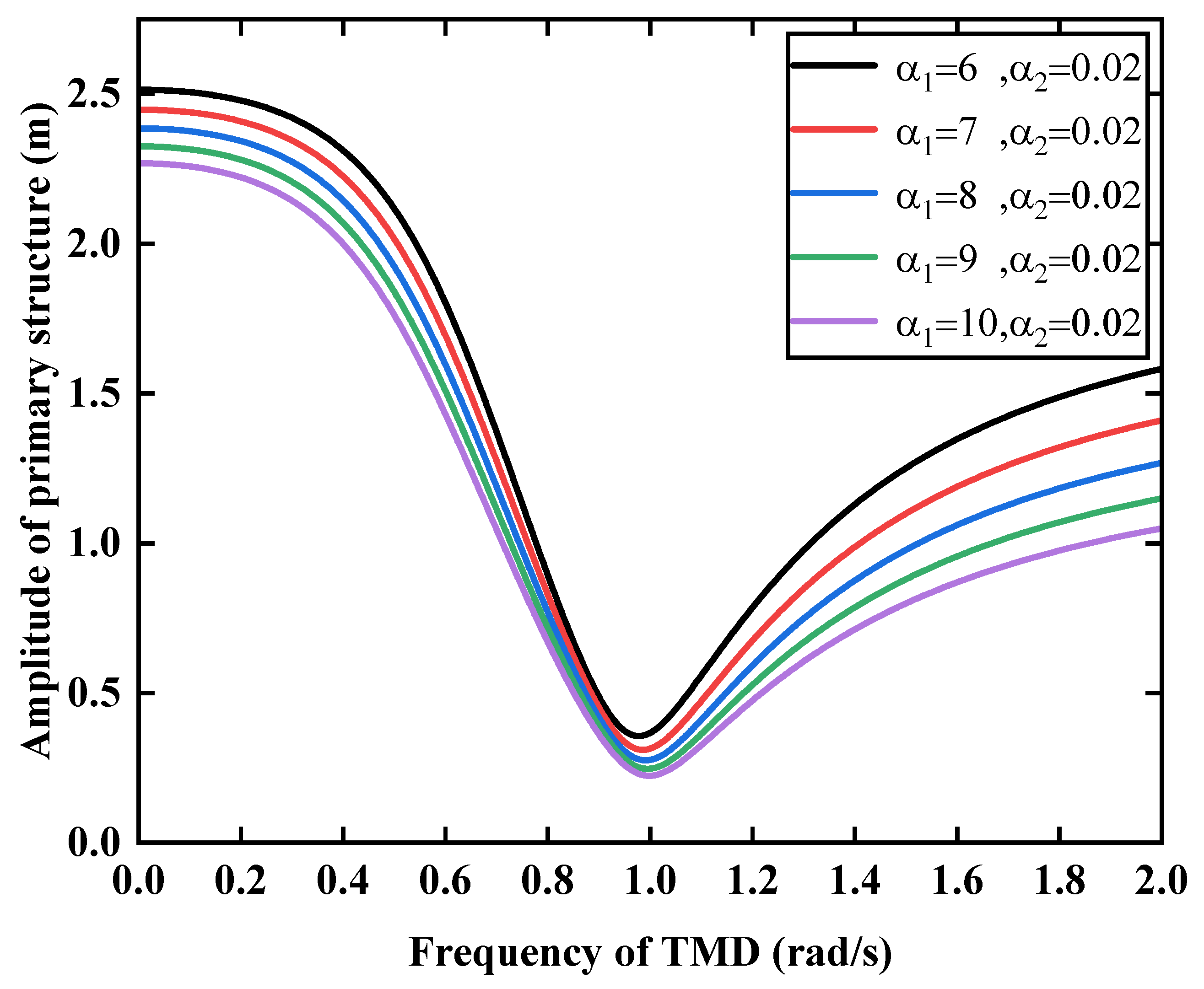Figure 11 shows a comparison of frequency–amplitude curves for NTMD and primary structure mass ratios of ${\alpha }_1=$ 6, 7, 8, 9, and 10. After the mass ratio of NTMD exceeded 10%, the improvement of the control effect for each 2% increase in the mass ratio of NTMD was not obvious, and too large of a mass ratio has influence on the control performance of the structure. In summary, the NTMD to primary structure mass ratio of ${\alpha }_1=$ 5 is more suitable.

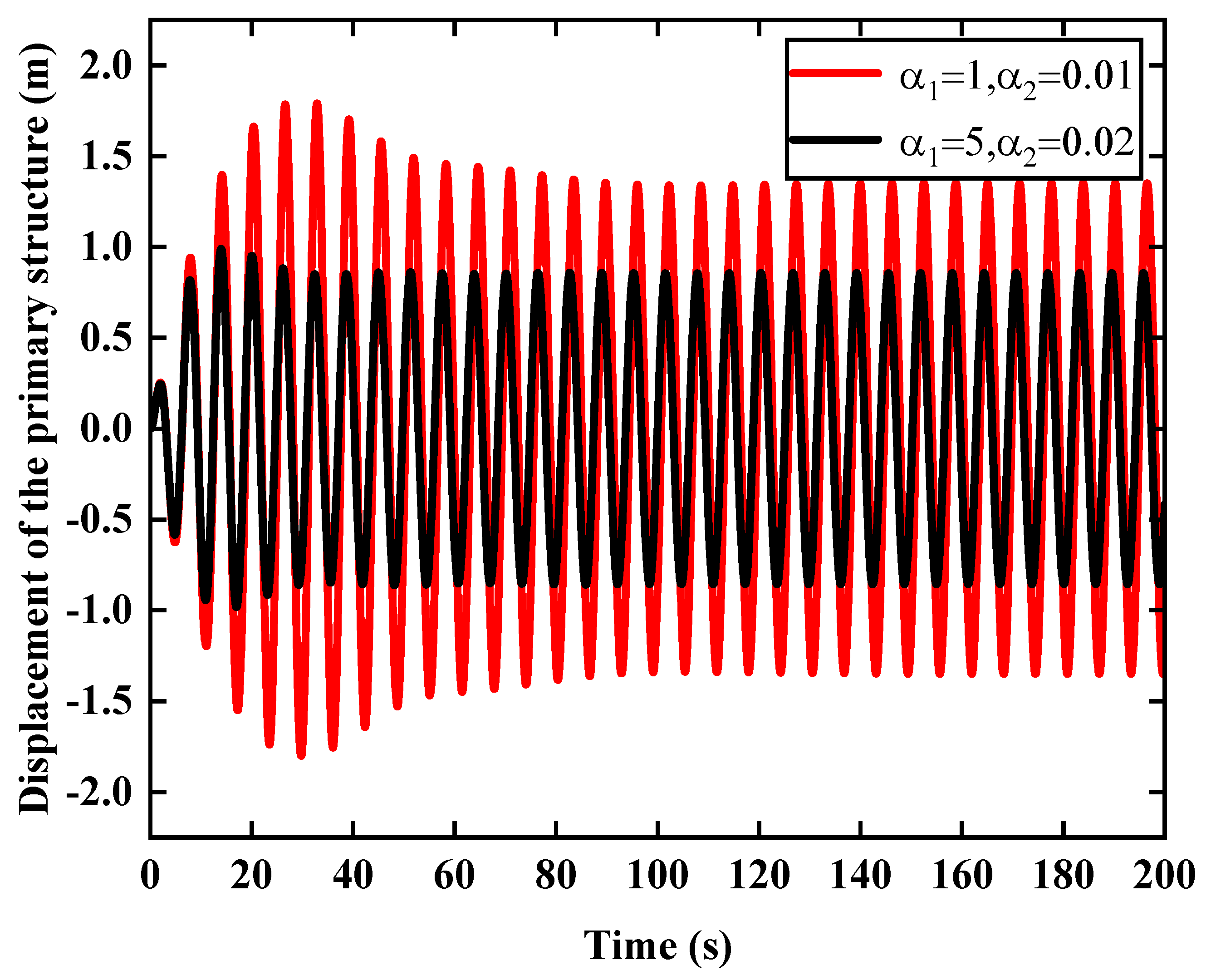
The response of the system was solved using the Runge–Kutta numerical integration method. The response characteristics of the solution were analyzed using a time course diagram for the parameter conditions of ${\omega }_2=$ 0.821, ${\alpha }_1=$ 5, and ${\alpha }_2=$ 0.02. As shown in Figure 12, the transient amplitude of the structure was reduced by about 44.75%, and the steady-state amplitude of the structure was reduced by about 36.62% compared to the initial design. The vibration reduction performance of the structure was effectively improved.

In summary, the optimal theoretical design parameters for a series of structures were obtained using the complex variable averaging method. Under these design parameters, the structural control performance was greatly improved, which provides a valuable reference for subsequent studies on the nonlinear characteristics of the TMD.

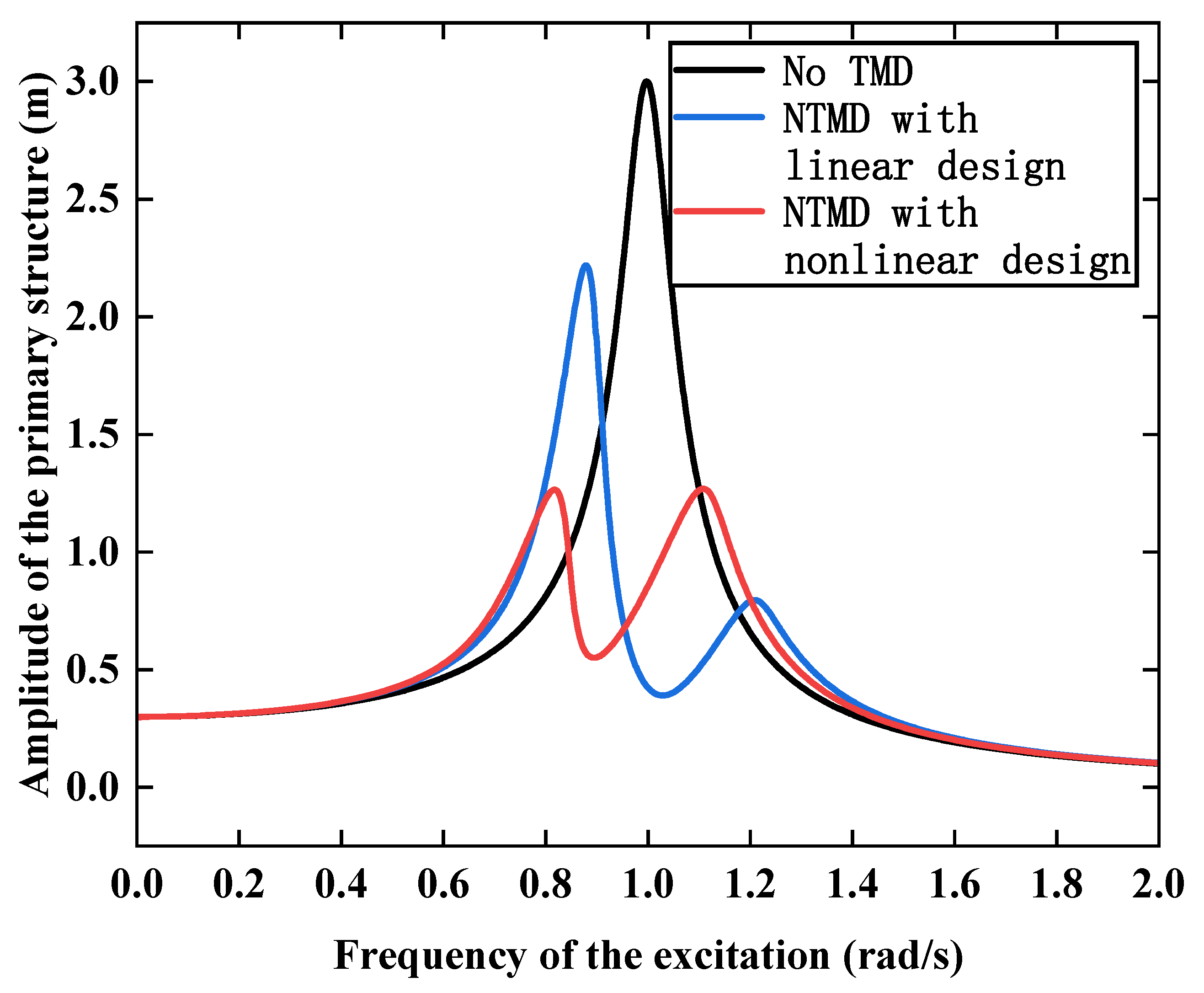
Figure 13 shows the frequency response curves of the primary structure with NTMD installed, designed using different methods. The frequency response curves allowed us to observe whether the steady-state amplitude of the structure decreased at different excitation frequencies after optimizing the NTMD. The black, blue, and red curves indicate the structures without TMD installed, NTMD with traditional linear design installed, and NTMD with nonlinear design installed. Figure 13 shows that the control performance obtained by using the traditional linear design method to optimize the NTMD was not satisfactory. The peak difference between the amplitude bimodal peaks was large, and the optimization effect was not good. In contrast, NTMD designed with nonlinear optimal parameters showed an equal amplitude at both left and right peaks. The control performance of the primary structure significantly improved compared to the linearly designed NTMD.

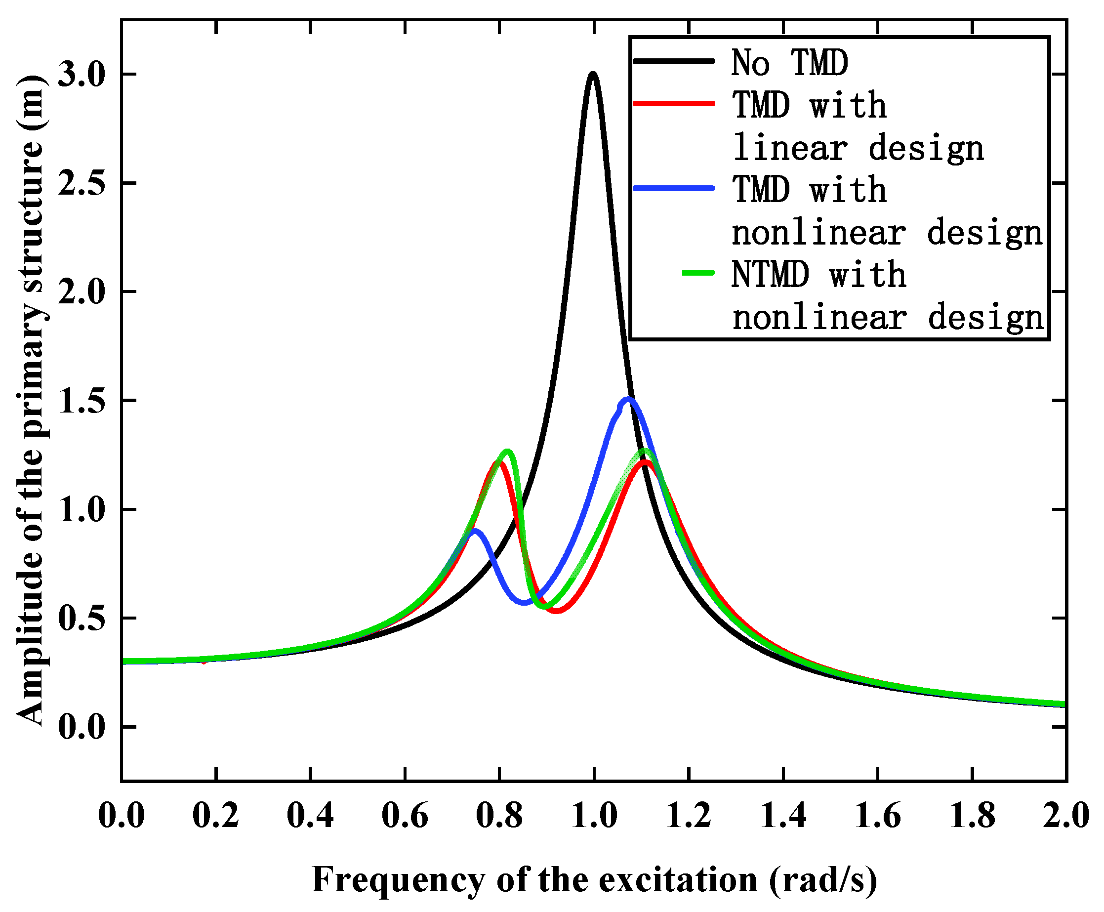
Figure 14 compares the control performance of the TMD and the NTMD. As shown in the figure, the red, blue, and green curves indicate the frequency response curves of the TMD with conventional optimal linear design, the TMD with nonlinear design, and the NTMD with nonlinear design, respectively. Compared to the conventional optimal linear design, the control performance of the TMD with nonlinear design was slightly weaker, but it still achieved nearly 58.33% of the optimized effect. Therefore, the nonlinear design conducted in the previous section is still valid for the linear TMD. As seen from Figure 14, the control performance obtained from the NTMD designed according to the nonlinear design method was comparable to that of the TMD designed using traditional linear design. Moreover, the TMD designed using traditional linear design and the NTMD designed using the nonlinear design method possessed 70.87% and 69.67%, respectively, of the optimization effect. However, the traditional linear design TMD was designed based on ideal cases and did not take into account the nonlinear characteristics of the TMD. On the other hand, the NTMD designed using the nonlinear design method was closer to engineering reality and had more reliable stability than the TMD designed using the traditional linear design.

The effect of the optimal nonlinear design NTMD on the vibration reduction of the structure is shown in Figure 15, where the amplitude of the primary structure in the steady-state phase was reduced by 71.47%. Figure 16 shows that the amplitude of the first-stage structure controlled by the ideal optimal linear design TMD was reduced by 75.43% in the steady-state phase, which is slightly better than that of the NTMD of optimal nonlinear design, but this is only the case where the TMD did not produce nonlinear characteristics. The comparison in Figure 13 shows that when the TMD produced nonlinear characteristics, the effectiveness of the linear optimal design parameters produced on the NTMD was greatly reduced.

In conclusion, the TMD optimization parameters obtained from traditional optimal linear design were only applicable to linear TMDs, and the optimization effect of TMDs decreased after nonlinear characteristics occurred during TMD usage. On the other hand, TMD optimization parameters obtained through nonlinear design had a good vibration reduction effect before and after the TMD produced nonlinear characteristics.

5. Computational Efficiency of Complex Variable Averaging Method and Numerical Method

In the previous section, the correctness and accuracy of the complex variable averaging method were demonstrated by comparing the results of the complex variable averaging method with those of the traditional numerical method. Under the premise that the computational results are guaranteed, the computational speed became an issue to be considered.

In practical engineering applications, the value added by the efficiency improvement to the overall project is undoubtedly huge. The complex variable averaging method was used to generate the frequency response curves of the primary structure, while the Runge–Kutta numerical method was used for comparison. The time required to generate the frequency response curves for both methods with the same parameter settings was recorded for 100 sets, and the first 10 sets of data recorded in

Table 2. Time required to produce a frequency response curve.

Complex Variable Averaging Method (s)	Numerical Solution Method (s)
1.410	84.660
1.214	84.741
1.194	86.348
1.258	85.767
1.280	85.461
1.119	85.721
1.291	86.285
1.332	86.488
1.122	85.789
1.176	84.689

are shown below.

From Table 2, the average time taken to generate the frequency response curve by the complex variable averaging method was 1.240 s, while the average time required by the numerical method under the same conditions was 85.595 s. The complex variable averaging method was significantly more efficient than the numerical method, saving about 98.55% of the time. The statistical results showed that the complex variable averaging method generates frequency response curves nearly 69 times faster than the basic numerical method, and it is able to obtain the steady-state solution quickly, saving a lot of time for the engineers designing the system.

6. Conclusions

This paper investigated the nonlinear behavior of tuned mass dampers during their operation. The system under study was a linear single-degree-of-freedom structure subjected to harmonic excitation and controlled by a TMD with hardening enhancement characteristics. The frequency response curves of the primary structure that was controlled by the TMD were obtained using an approximate analytical method. The study presented in this paper can be divided into three main parts, which include the following contents and conclusions:

• The correctness and accuracy of the approximate analytical solution were verified by comparing with the conventional numerical methods. The steady-state displacement amplitudes of the primary structure were calculated under the control of a TMD that took into account the nonlinear characteristics of the stiffness. The results showed that the design of the TMD, considering such nonlinear characteristics, can help to improve the control performance of the structure by the TMD.
• The effects of different system parameter variations on the shape of the frequency–amplitude curve and structural stability were investigated, and the optimal design parameters of the system for a specific case were given. The results showed that the optimal nonlinear design NTMD had almost the same control effect as the traditional optimal linear design TMD. However, the nonlinear design NTMD had good vibration reduction performance in different cases and was closer to engineering reality. It had a certain reference value in subsequent studies of the nonlinear characteristics of the TMD.
• Frequency response curves generated by the Runge–Kutta numerical method and the complex variable averaging method under the same parameter conditions were compared. The statistical results showed that the complex variable averaging method generated curves nearly 69 times faster than the Runge–Kutta method and could quickly obtain the structural steady-state solution, saving time for system designers. The use of analytical methods can improve efficiency in practical engineering.