1. Introduction
The main reasons for the failure of the steel components and pipelines at nuclear power plants are the defects that appear during the manufacturing processes or operation. The defects usually are cracks that appear due to material degradation mechanisms such as stress corrosion cracking (SCC), fatigue, or others. Material, stresses, and environment are the three factors that should be present in order for SCC to initiate. All these factors are important and, in some cases, could lead to the formation of a crack [
1,
2]. This kind of defect usually appears in pipe welds at heat-affected zones. Undetected and unevaluated cracks are very dangerous because they can lead to fast failure or even to the guillotine break of the pipelines and other pressure vessels at relatively low loading conditions. Therefore, it is very important to detect and evaluate these defects. Casting, rolling, bending, pressing, stamping, welding, and other manufacturing processes lead to the accumulation of residual stresses which also have to be taken into account. It is known that residual stresses affect crack growth rates [
3,
4,
5] and the durability under the effect of cyclic loading [
6,
7,
8,
9,
10]. Residual stresses and weld defects together have critical and risky effects on the structures. The static residual stresses have an influence on the life of components under fatigue loading conditions. These variations are introduced in both initiation and growth of fatigue cracks [
11].
SIF is important for the evaluation of crack initiation and growth. Cracks usually appear in the weld seams or heat-affected zones where welding residual stress is present. Acting operational stresses together with residual stress could lead to unpredicted/premature weld seam failure. Therefore, it is important to know how the residual stress affects crack initiation and growth in the structural integrity analysis of weld seams. In this research, thermal loading was applied to the finite element (FE) model for the introduction of residual stress and evaluation of their influence on SIF values.
Despite the significance of residual stresses, there has not been much research on the effects of combining crack closure mechanisms with residual stress distributions during crack propagation. Since both tension and compression stress values are present across the thickness, the crack closure can be described using the polynomial equation [
7]. The main reasons for the rare investigation of the residual stress effect could be the difficult and long-lasting experimental stress measurements. Furthermore, it is difficult to predict the residual stresses accurately that arise from manufacturing procedures. Typically, in such cases, a nonlinear FE analysis is used. Due to the lack of accurate residual stress data in the components and structures, the integrity analysis based on fracture mechanic analysis is usually limited or too conservative. As a result, residual stress-bearing structures’ structural integrity is evaluated cautiously, frequently, and very conservatively which frequently forces safe equipment out of service earlier than necessary and at a large expense [
12].
According to this, it is important to estimate the influence of the residual stress on the behavior of defects in welded structures. Lee and Chang [
13] using FEA analyzed how the defects in welds affect the cylindrical steel members structurally. As a result, non-axisymmetric buckling was determined close to regions with defects caused by an asymmetric distribution of residual stress. Labeas and Diamantakos [
14] evaluated the weld residual stresses for cracked T-joints welded with a laser beam and calculated the stress intensity factor (SIF) using FEA with different crack shapes. The damage tolerance methodology was used for the determination of the weld joint’s remaining lifetime. Lee and Chung [
15] conducted a numerical non-linear 3D analysis to determine the residual stresses on welds of similar as well as dissimilar metals. It was concluded that the difference between the longitudinal residual stresses increases together with the yield strength of the parent materials in dissimilar steel welds. Wu [
16] evaluated the residual stresses effect on a surface crack with a brittle fracture behavior. He recommended a post-heat treatment to relax the residual stress in the weld joints.
In trying to understand what influence makes residual stresses on austenitic stainless steels and how they interact with the initial level of pre-straining, research work was carried out in the CEA Saclay, France [
17]. The SCC resistance of the initially pre-strained plate (from 30% to 60%) was analyzed in these experiments. To carry out such an experiment, the CT specimen was machined from the pre-strained plate. Before the SCC test, a fatigue pre-cracking is performed on each specimen. At the end of the SCC tests, the CT specimen was completely broken by using the testing machine. The fracture surface revealed a particular fatigue crack with a smaller propagation at the center of the specimen and no SCC crack growth at this location, whereas significant SCC propagation has been obtained near the edges.
The numerical simulation of the stress intensity factors along the crack front of the CT specimen was carried out. Usually research is made for a not pre-strained material on a specimen with an initial straight crack front or machined notch, and the higher values of the stress intensity factor are observed in the middle of the specimen and lower values are observed at the sides of the specimen: a larger crack growth in the middle of the specimen is then expected, which was not the case here. However, in the case when the plate was initially pre-strained (plate with residual stresses), it seems that an opposite distribution of stress intensity factor along the crack front is observed: the higher values were at the sides of the specimen and the lower ones were in the middle. It was also justified by the obtained crack shape after pre-cracking.
The main goal of this paper is to numerically evaluate how the residual stress affects the SIF profile at the crack front. To achieve the main goal of the research, the following tasks should be conducted:
create the residual stress profile in the numerical model by adding a temperature profile;
apply the created residual stress profile to the standard CT specimen model;
compare the numerically determined SIF profile in cases with and without residual stress.
To accomplish the previously described tasks, the computer program Cast3M was chosen [
16]. This program is based on the FEM which is validated for the calculation of fracture parameters such as SIF and J-integral. To make this research close to a real-life scenario, the experimentally determined material properties and the measured residual stress profile of highly pre-strained stainless-steel plates were used. The experimental tests and FE simulation were conducted at an elevated 325 °C temperature.
The analysis results of this research show how residual stresses affect the SIF profile along the crack front and that these stresses have a bigger influence on the surface rather than the central part of the specimen. As the secondary goal of the paper, the method for residual stress application to the FE model was demonstrated.
2. Initial Data for FEA
The preparation of specimens, mechanical properties, and all the experiments were carried out at Atomic Energy Research Center (CEA Saclay), France [
17].
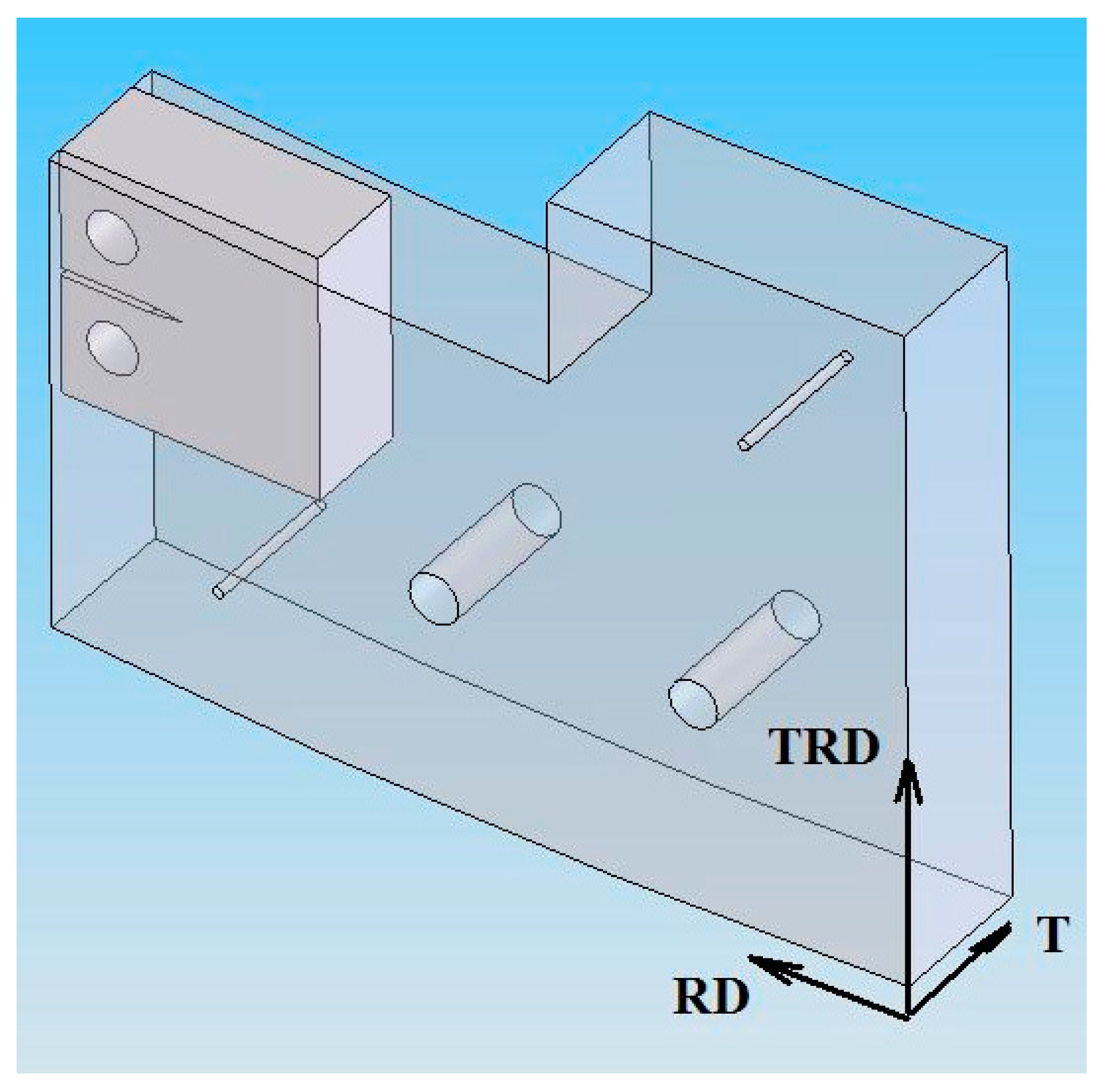
The tests were made using the CT specimen machined from a pre-strained 316 L stainless steel plate. The plate was pre-strained at about 40% in the T (transverse) direction (see
Figure 1). Pre-straining was made by rolling in RD direction (rolling direction). TRD (transverse rolling direction) is a perpendicular direction to RD. Due to rolling at a high strain level, the otherwise straight plate was curved, where one surface of the plate became concaved and the other—convexed. The plate thickness after rolling was ~20…21 mm and the machined CT specimen’s thickness was 15 mm.
The same plate was used for residual stress measurement performed by Bristol University [
17] using their developed deep hole drilling (DHD) technique [
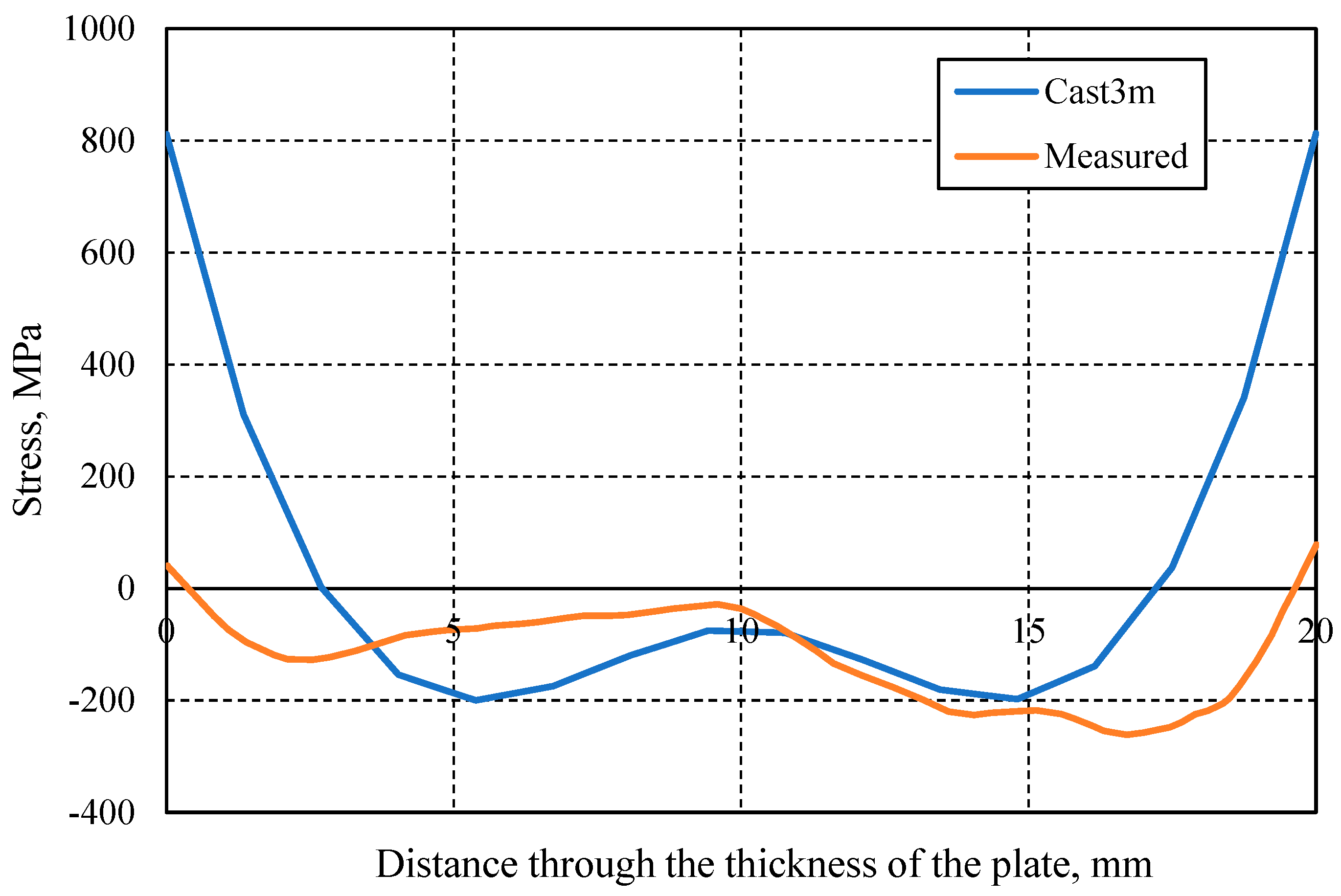
18]. The measurement technique consists of four steps. Initially, a small diameter hole is drilled through the thickness of the measured specimen. The second step is the accurate measurement of the diameter of this hole at many depths and angular points. After that, the material around the hole is freed coaxially using a coring tool. The last step consists of the measurement of the hole diameter at the same measurement points as in the second step. The measured distortion of the diameter is later used for the determination of residual stress. Measured residual stress profiles are shown in
Figure 2. The figure shows the residual stress distribution along the thickness of the plate in RD and TRD directions. The distance of 0 mm is on the convex surface of the plate (see
Figure 3) and the distance of 20 mm is on the opposite (concave) surface. The measurements show the higher residual stresses are in TRD, the same direction CT specimen tension, and crack opening is simulated. Therefore, residual stresses in TRD will be taken into account in this analysis.
The tensile testing of 316 L stainless steel was made at 325 °C. The location and orientation of the tested tensile specimens in the plate are shown in
Figure 3. Two columns with six specimens in each column in different plate depths were prepared. In total, twelve 2 mm thickness specimens were tested. The averaged material properties are as follows [
17]:
Modulus of elasticity E = 176,360 MPa,
Poisson’s ratio ν = 0.3,
yield stress Rp0.2 = 655 MPa,
cinematic stress hardening H = 20 GPa,
thermal expansion coefficient α = 1 × 10⁻⁵/°C.
3. Residual Stress Modeling
The original stainless-steel plate was pre-strained by rolling at very high ratios (between 30% and 60%). In fact, the pre-straining was not homogeneous through the thickness, which generated a residual stress profile to ensure strain compatibility. In this paper, the focus will be on the plate pre-strained at 40%.
There is no straightforward method for residual stress application at the numerical model in most FEA codes. It is not always possible to obtain a correct distribution of residual stresses using only external mechanical loading, such as force or pressure. That is why, in this case, thermal loading was used. It was based on the assumption that thermal loading and residual stresses are equivalent to the imposed strain loading conditions. The change in the temperature compared to the base temperature makes the material expand or contract. The amount of expansion is described in the material model by the thermal expansion coefficient. Temperature itself cannot induce stress or strain if the expansion or contraction of the material is not restricted. Only then, if the expansion or contraction is restricted, can the strain in the material appear. The restriction in the model can be applied by the boundary conditions or by the opposite thermal load similar to the forces acting in opposite directions. According to this, we applied the temperature profile to the model in such a way that the induced stress profile was similar to the measured residual stresses. In addition, this obtained stress profile was used for the evaluation of residual stress influence on SIF.
The main challenge of thermal load application is to find the correct temperature profile distribution through the thickness of the plate which leads to a similar residual stress distribution that was measured experimentally. The next step is to run the CT specimen tension simulation for SIF calculation by applying the defined temperature distribution.
For the determination of the thermal profile for residual stress application and SIF calculation, the FE code Cast3M was used. This code was developed in DEN/DM2S/SEMT CEA Saclay, France and is used for solving various problems, especially for fracture mechanics [
19].
3.1. FE Model for the Residual Stress Modeling
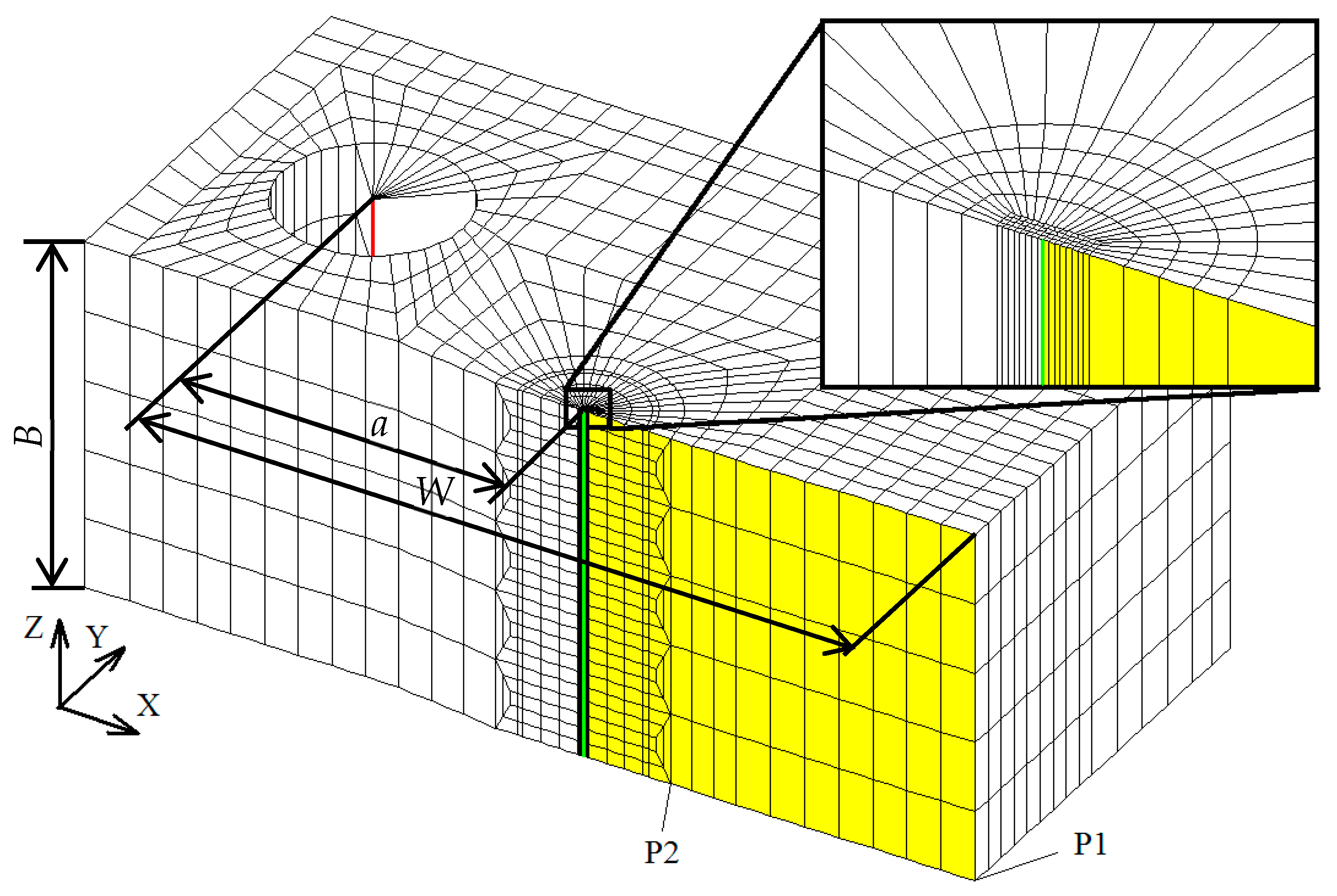
To find the correct temperature distribution along the thickness of the steel plate, the FE model of the 20 mm thick plate was made (see
Figure 4). The modeled steel plate was three times bigger than the CT specimen and its dimensions were 90 × 90 × 20 mm. The three-dimensional cubic elements CU20 were used for the mesh of the plate which have 20 nodes.
For the residual stress distribution calculation, an elastic analysis was conducted. Therefore, to describe the material only, the modulus of elasticity, Poisson’s ratio, and thermal expansion coefficient presented in
Section 2 were used.
The following boundary conditions of the model were applied: the displacements of point P1 were restrained in all three directions; the displacement of point P2 was restrained along the
Z axis; the displacement of the yellow-colored surface was restrained along the
Y axis (see
Figure 4).
The red-colored line is the line where the stress profile was measured.
3.2. Results of the Residual Stress Modeling
To find the correct temperature profile which results in a stress profile similar to the measured one (
Figure 2), several calculations were conducted. As was explained in
Section 3 in order to induce stress using thermal loading, the temperature profile should have lower and higher values according to base temperature. For convenience, the base temperature of the material was selected to be equal to 0 °C which is a temperature at which no stresses are induced. The measured residual stresses have the compressive and tensile stresses, therefore, the thermal load should also have lower and higher values compared to the base temperature equal to 0 °C. In our case that would be negative and positive temperature values. Positive thermal load values force the material to expand. Without restriction, only the dimensions of the model would increase, and no stresses would appear. The restrictions to the expansion of the material were applied by negative temperature values. The restriction to the expansion of the material induces compressive stress, and vice versa, restriction to the contraction of the material induces tensile stress. That is why the temperature profile should look somewhat like a mirror image of the residual stress profile in respect to the abscissa of the graph. Moreover, to avoid the warping of the model temperature profile, there should be symmetry along the middle plane of the model.
Taking into account all the statements, the above temperature profile was constructed. The actual temperature values were adjusted by running several FE analyses and comparing the calculated stress profile with the measured residual stresses.
The best temperature profile found is shown in
Figure 5. The figure also shows the trendline and a polynomial equation describing the profile. The best-fit temperature profile shows the lowest temperature values up to −200 °C on the surfaces of the plate, and the highest values up to 200 °C in 5.5 mm depth from both surfaces of the plate.
The found temperature profile was applied to the plate as the loading (see
Figure 6). The temperature was applied to all nodes of the model where the temperature value for each node was calculated according to the following equation:
here,
T—temperature, °C; z—z coordinate of the node, mm.
Von Misses stress distribution due to the temperature loading is shown in
Figure 7 and the stress profile in TRD is shown in
Figure 8. The obtained stress profile has the simplified shape of the measured residual stress profile. The lowest stress values are −200 MPa; in the very middle of the plate, the stress value is −50 MPa and the highest values are up to 800 MPa on both sides of the plate. As we are interested in SIF calculation, evaluating residual stress in the CT specimen, which is 15 mm thick in the very ends of the stress profile, is not important. The 2.5 mm of the plate from both sides as well as the thermal loading profile will be cut out. Moreover, the exact match of the residual stress of the profile is not relevant in the current study because the final results, i.e., SIF profile, will not be measured with experimental data, but only with the numerically determined SIF profile in cases with and without residual stress profile. It is because standard procedures for experimental determination give an average value of SIF through the thickness of the specimen but not a profile.
To find out what the residual stress profile will be in the CT specimen when the cut out thermal profile is applied to the model, the calculation was performed, and the results are presented in
Section 4.2.
5. Conclusions
In the current research, the following analyses were conducted:
residual stress modeling by finding the temperature profile which leads to the stress profile similar to the measured;
stress intensity factors in CT specimen calculation and comparison at loading cases with and without residual stresses.
The results of the analysis have shown that in particular cases, the residual stresses can lead to a situation where the values of the stress intensity factor at the middle of the specimen are lower than at the sides. That should be taken into account when surface cracks and their propagation is evaluated. Moreover, in the analyzed case, residual stresses have reduced the average value of the stress intensity factor. However, in the case of different residual stress profiles, the result could be the opposite, i.e., the average stress intensity factor value could be increased due to residual stresses, which is usually observed in weld seams. Therefore, residual stresses should always be evaluated and cannot be neglected.
The methodology of this analysis can be used in the structural integrity evaluation of defects in metal components with residual stresses. It is important to note that the methodology is designed to create a residual stress profile using temperature as loading and evaluate the influence of residual stress on SIF. The calculation accuracy is very much dependent on the correct thermal load profile determination. As it does not allow for determining the residual stresses numerically, great attention should be paid to the residual stress measurement, thermal load determination, and model calibration. The main drawback of the method is the destructive nature of residual stress measurements. To improve that, new non-destructive methods should be used.


