Article

Directional Amplification at Rock Sites in Fault Damage Zones

1
Istituto Nazionale di Geofisica e Vulcanologia, Sezione Roma 1, Via di Vigna Murata 605, 00143 Roma, Italy
2
Dipartimento di Scienze della Terra, Università Roma Tre, 00146 Roma, Italy
3
US Geological Survey, 345 Middlefield Road, Menlo Park, CA 94025, USA
4
School of Geography, Environment and Earth Sciences, Victoria University of Wellington, Wellington 6012, New Zealand
*
Author to whom correspondence should be addressed.
Appl. Sci. 2023, 13(10), 6060; https://doi.org/10.3390/app13106060
Submission received: 9 March 2023 / Revised: 4 April 2023 / Accepted: 14 April 2023 / Published: 15 May 2023
(This article belongs to the Special Issue New Challenges in Seismic Hazard Assessment)

Abstract

:

Featured Application

In the seismic design codes of many countries, site amplification effects are accounted for through the use of scaling factors due to the presence of superficial soft soil deposits. In this framework, rock sites are assumed to show no local amplification. However, even rock sites can show site amplification, and the presence of large-scale open cracks or microcracks can affect large areas, such as across fault zones and on landslides. The existence of unexpected site-effects at rock sites can have significant implications in seismic hazard assessment. The current-knowledge is limited to relative amplification between horizontal and vertical components, and further estimates are needed in order to evaluate the absolute amplitude and to understand to what extent this effect could be important for seismic hazard and engineering applications.

Abstract

Site effects refer to the modification of ground shaking caused by the local geological conditions that can result in the strong amplification of ground motion. The best-known cause for site effects is the presence of superficial soft soil deposits, which are considered in seismic design codes of many countries through the use of scaling factors. Rock sites are assumed to show no local site amplification. However, even at rock sites, seismic waves can be locally amplified at frequencies of engineering interest, with larger motion along one site-specific azimuth on the horizontal plane (the so called “directional site resonance or amplification”). These effects have been related to the presence of large-scale open cracks or microcracks in different geological environments (faults, landslides, volcanic areas) everywhere with a common signature: maximum amplification occurs transverse to the predominant fracture strike. In this paper, we summarize our main results obtained in the last decade with regard to several fault zones with different kinematics, where ground motion is polarized (and amplified) perpendicularly to the predominant fracture field as an effect of the stiffness anisotropy. In order to give a further constraint, we also show some cases where the directional amplification effects were compared with the S-wave splitting analysis method.

1. Introduction

Recently, directional amplification (DA) effects have been widely observed worldwide, with wavefield polarization at a high angle to the fault strike. Using an expression proposed by [1], DA implies that the Fourier spectra of the two horizontal components do not show the same amplitude levels, but rather there is a preferential direction of amplification, reported as a strike from the geographic North. In the time domain, DA effects correspond to linearly polarized ground motion, with mean polarization along the same direction. Seminal papers with observations of DA date back to the early 2000s (e.g., [2,3,4,5,6]). Since these effects appear at low frequencies (even lower than 1–5 Hz), they cannot be related to the superficial rock layer affected by the weathering processes. Furthermore, the high-angle of the polarization compared to the fault strike suggests that they cannot be interpreted as fault trapped waves; trapped waves yield a large motion of amplification parallel to the fault strike [7,8,9,10,11,12,13,14,15].
Pischiutta [16] studied the directional amplification effects in a wide range of faults, concluding that the polarization of amplified motion is perpendicular to the strike of the predominant fracture field expected from modelling. They proposed that in fault zones the ground motion is polarized (and amplified) perpendicularly to the pervasive fracture fields, held open by the favourably-oriented stress field. Differences among faults in the angle between maximum amplification and fault strike mainly reflect differences in fault kinematics responsible for fracture attitudes. Pischiutta [17] demonstrated that directional amplification was not related to the seismic source and path, therefore it is necessarily ascribed to a local site effect.
Several following works that also involved direct comparisons with measured minor faults/fracture orientations measured in the field, confirmed that interpretation [18,19,20,21,22,23,24,25,26]. Similar conclusions were also achieved for large open cracks observed in landslides [27,28,29,30,31,32]. This interpretation was also confirmed through the comparison with S-wave splitting analysis [23,33,34]. Fractured rocks cause (i) ground motion polarization and directional amplification, and in the fracture-perpendicular direction as an effect of stiffness anisotropy, and (ii) velocity anisotropy with Vs (shear wave velocity) larger in the fracture-parallel component.
Finally, in a recent paper, [35] demonstrated the capability of fractures in the shallow subsoil to reorient signal polarization though a controlled-source seismic experiment. They employed a vibratory source capable of producing harmonic vibrations, finding that the ground transmitted energy more efficiently along the azimuth of maximum amplification independently of the original source polarization transmitted in the ground.
In this paper, we show the main results that we obtained in the last decade across different fault zones characterized by different geological and lithological settings, as well as by different kinematics. The goal is to provide an organic summary of our work about the occurrence of directional amplification effects and ground motion polarization across fault zones.

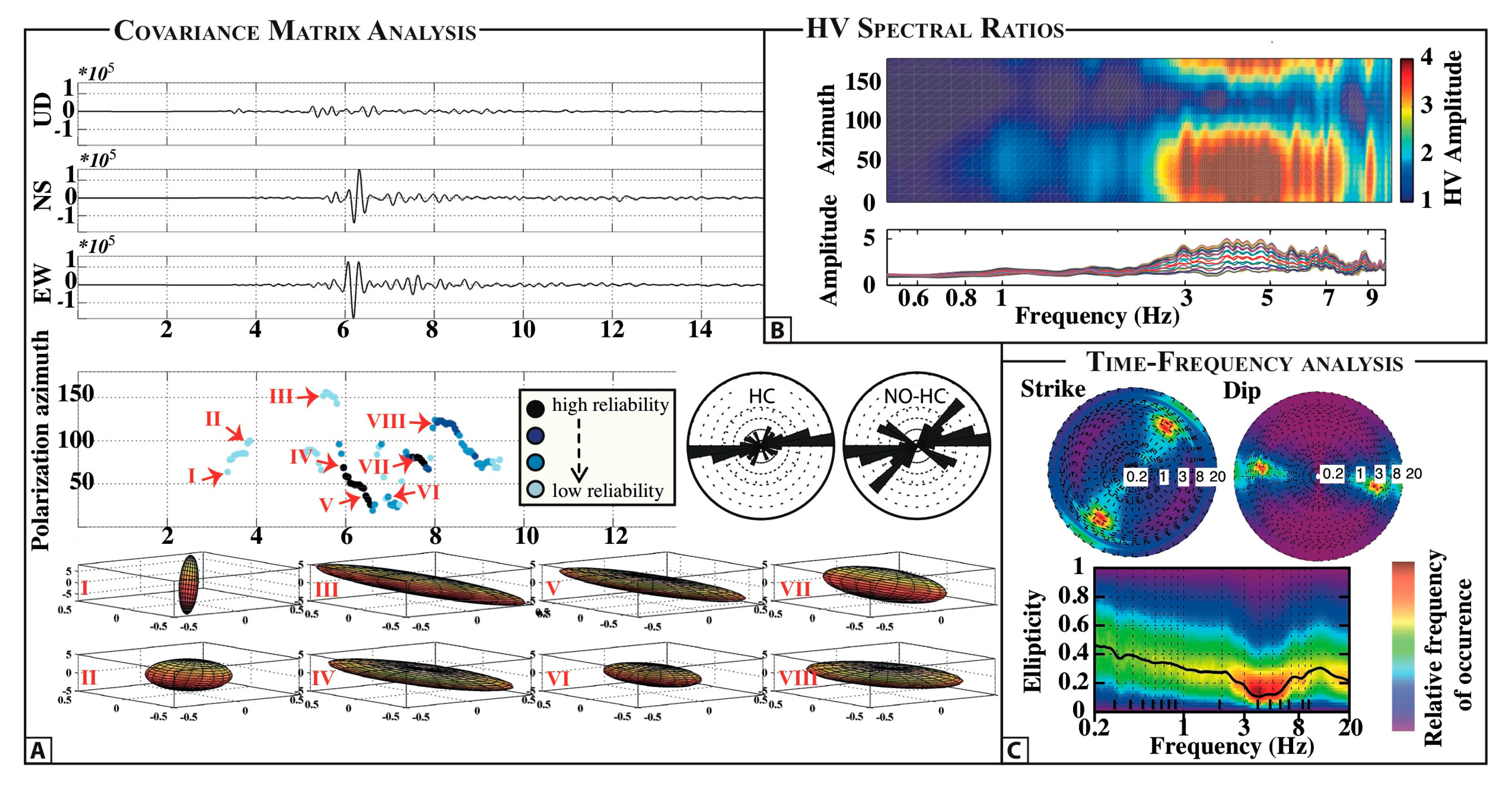
2. Methods of Analysis

The methods adopted to assess ground motion polarization and directional amplification to this point have involved the use of the ambient noise wavefield and earthquake data.
The oldest technique to get information on amplification-prone sites is based on the spectral ratios SSRs (standard spectral ratios) ([36,37], and later papers) of horizontal ground motions recorded during an earthquake at close sites with different near-surface geological structures. SSRs require the presence of a reference site not affected by any site amplification effects. Therefore, its use is somewhat suspect when studying tectonically active areas where it is difficult to find a reference site in the proximity of the studied fault zone sector. Therefore, it is not applied in the present study. In a similar approach, another technique involves the calculation of spectral ratios between horizontal and vertical components (HVSR), generated by earthquakes or ambient seismic noise at individual stations [38,39]. The theoretical basis of this method is still debated [40]; however, it is a very efficient tool for mapping the different seismic motions of nearby sites. When dealing with the ambient noise, DA might be caused by many factors, such as the local geological setting or the sources of the ambient noise. For example, [41] observed the DA in the frequency band 0.15–0.6 Hz, finding that the location of the sources affects the polarization of the ambient noise [42].
In order to identify directional amplification, both SSR and HVSR are calculated by rotating the two horizontal components. The use of rotated spectral ratios was first introduced by [43] and was subsequently exploited by several authors to detect the horizontal polarization of ground motion in fault zones (e.g., [4,5,16]). When using seismic events, both SSR and HVSR values are calculated at each station separately for each event, considering a portion of the signals with a varying length (depending on the event magnitude), but always including the S and early coda waves. The spectra of horizontal motions are computed after rotating the NS and EW components by steps of 10°, from 0° to 180°. A taper (i.e., Hannning) and a smoothing filter (such as a running mean box or triangular filter; or a Konno-Ohmachi filter) [44], are generally applied. The spectral ratios are then graphed, calculating the mean over the considered seismic events.
An example of an HVSR calculation is shown in Figure 1B, clearly showing the amplification in a broad frequency band (from roughly 3 to 7 Hz), with amplitudes over a factor of 4; amplification is the maximum for the N40° rotation angle (NE-SW).
Because the spectral ratios (SSR and HVSR) may be biased by anomalies in the spectrum of the vertical component (at the denominator), in the time domain the covariance matrix method [45,46] has been widely exploited to estimate the ground motion polarization (e.g., [5,6]). The covariance matrix is calculated using overlapping moving windows (the length tailored on the basis of the predominant signal frequencies). The eigenvalues and eigenvectors are determined by solving the algebraic eigenproblem and through the code POLARSAC [47,48,49]. They correspond, respectively, to the axis length and to the axis orientation of the polarization ellipsoid that represent the particle motion in the data window. The polarization azimuth is the angle between the projection of the largest eigenvector on the horizontal plane and the geographic north. Further details about the covariance matrix analysis can be found in Section 1, and in [17] Appendix A.
In Figure 1A, an example is given, reporting: (i) filtered signals of the three components of ground motion; (ii) eight examples of polarization ellipsoids with different shape (elongation, horizontality, and flatness) and related to different seismic phases; (iii) values of polarization azimuth (i.e., the projection on the horizontal plane of the eigenvector associated to the maximum eigenvalue) versus time. The employed color scale related to the reliability scale is based on the hierarchical criterion as introduced in [34]. We show two rose diagrams in order to show the influence of the application of this hierarchical criterion on the final representation of ground motion azimuth results (1).
Another widely exploited technique is represented by the time—frequency (TF) polarization analysis, proposed by [50] and used by [28]. This technique can provide quite robust results, overcoming the bias that could be introduced by the denominator spectrum in the SSR and HVSR calculation. In Figure 1C, we show some examples obtained through the code Wavepol written by J. Burjanek. An ellipticity plot vs frequency gives an indication about possible linear polarization, this parameter being close to 0 for linearly polarized ground motion. Moreover, the polarization strike and dip obtained all over the time series analyzed are represented using polar plots, where the distance to the center represents the signal frequency in Hz, and the contour scale is related to the relative frequency of occurrence of each value. In the same frequency band where HVSR shows amplification, the ellipticity reaches its minimum values (under 0.2), indicating linearly-polarized ground motion (Figure 1C). Moreover, the strike polar plot shows polarization between N40° and N50°, consistent with the HVSRs. Finally, the dip polar plot confirms that the ground motion polarization is concentrated on the horizontal plane, with predominant values between 90° and 100°.
The performance in the use of these three techniques to constrain directional amplification was recently tested on Ischia Island by [51], through over 70 ambient noise measurements. They confirmed coherent outcomes.

3. Results

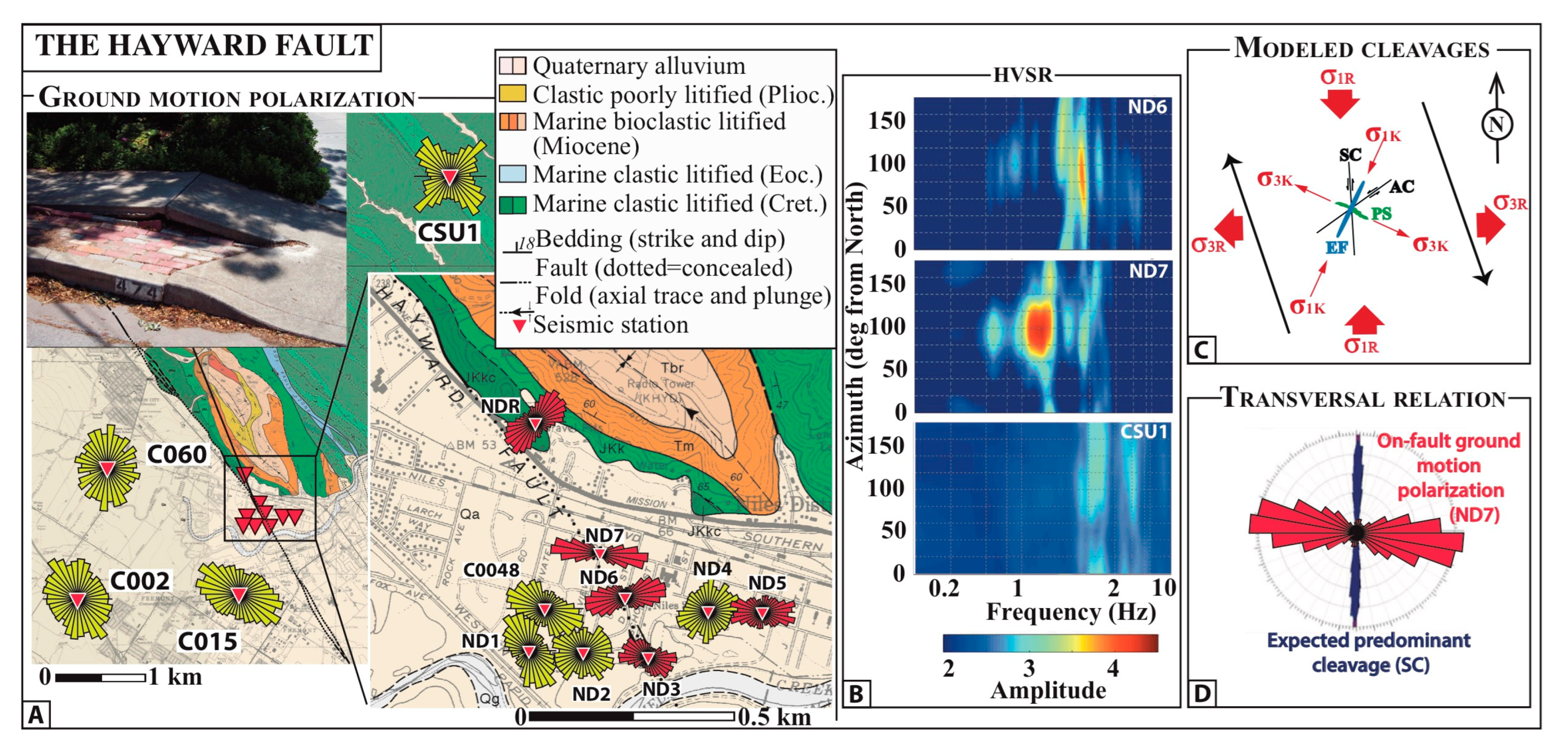
3.1. The Hayward Fault Case Study

Ground motion polarization in the Hayward fault zone was recently investigated [17]. The Hayward Fault (HF) is located just east of San Francisco (CA), and shows a quite complex structure with a general trend of N340°, a predominant strike-slip right- lateral movement, with 100 km offset during the past 12 Ma [52,53]. Both geomorphic evidences and offsets of man-made structures adequately document the active surface trace of the HF, revealing that it has a significant creep [54,55]. In spite of this, the fault has also shown moderate to large earthquakes (ex. the ∼6.8 magnitude earthquake in 1868) [54,55,56,57]. The study area is located in the Fremont district near Niles Canyon, where the highest surface creep rate is observed and the HF is largely aseismic. In the eastern fault sector, several marine clastic sequences outcrop, while the western sector is characterized by the presence of Quaternary alluvium. The geological map (downloaded at https://ngmdb.usgs.gov/, last accessed on 16 May 2021) is reported in Figure 2A. On the top-left, we also show a picture taken close to station ND6, showing the damage on a concrete sidewalk made by the fault creeping movement.
Ground motion polarization was investigated in [17] by using earthquake waveforms recorded by a temporary accelerometric seismic array installed by the US Geological Survey across the fault. Their location is shown in Figure 2A. Stations were installed at small distances (hundreds of meters) across the fault, and operated between 2006 and 2013 (details about the data set can be found in Table 1 in [17]). In this work, we have extended the performed analysis, adding six additional stations (Table 1) installed in the same area and belonging to Northern California Seismic Network (NCSN). Since these stations were operating in different periods, we performed a further data selection using IRIS Wilber3 tool (http://ds.iris.edu, last accessed on 19 April 2021), selecting data with a magnitude higher than 3. The details can be found in Table S1, given as auxiliary material. We used the covariance matrix method applied to the three component records. The results obtained from the selected earthquake are combined, merging all the instantaneous polarization angles. In Figure 2A we show the horizontal polarization at each station through rose diagrams, merging the polarization angles of all of the events. The four on-fault stations have narrow rose diagrams, implying horizontally polarized motion: polarization at stations ND6 and ND7 is along the N80°–90° direction; at ND3 the pattern is more complex, with two effects at different frequencies (the N80°–90° direction only in the frequency band of 6–8 Hz, see also [7]); at NDR the polarization slightly rotates to N70° azimuth.
Conversely, off fault stations (ND1, ND2, ND4, C002, C015, C060) show rose diagrams with scattered polarization angles, with no clear prevailing direction.
The mean HVSRs averaged over the selected events are shown in Figure 2B for three selected stations (further details of the analysis can be found in [13]).
The off-fault station CSU1 shows low HVSR amplitude levels that do not reach a factor of 3. Conversely, at the two on-fault stations (ND6 and ND7) the horizontal motion exceeds the vertical one with peak values up to a factor of 4.5 in the frequency band of 1–7 Hz. Moreover, the amplitudes at peaked frequencies show a distinct variation as a function of the rotation angle, with maximum amplification along the N80–90° azimuth.
The source polarization was modeled in [17] for direct P and S waves using the software ISOSYN [58], in order to verify whether this polarization effect could be ascribed to the seismic source. However, the modelled source polarizations did not agree with the observed one on direct body waves, implying that polarized motions at on-fault stations were not controlled by the source properties but rather due to local site effects.
The polarization effect in the fault zone was interpreted by [17] in terms of fracture fields. The direction of the fracture cleavages expected for the HF was calculated using the package FRAP [59] (see the Appendix A in [17]). The model results suggested that for this fault kinematics, the predominant fracture cleavage is represented by synthetic cleavages (i.e., Riedel shear), that here develop with a mean azimuth of N4° (the blue rose diagram in Figure 2D). To help a correlation with ground motion polarization, the combined results from the analysis of seismic events at stations ND6 and ND7 are also plotted (red rose diagram).
Based on these findings, Ref. [17] proposed that in the studied sector of the HF, the horizontal polarization of ground motion is orthogonal to the orientation of the most probable fracture system (synthetic cleavage).
In Figure 2C, we provide a sketch of a map view with the regional stress field (red arrows), the right-lateral fault movement in the N160° direction (black arrows), and the kinematic components of the local stress field (K1 and K3). The expected fracture systems (cleavages and extensional fractures) are illustrated as well.

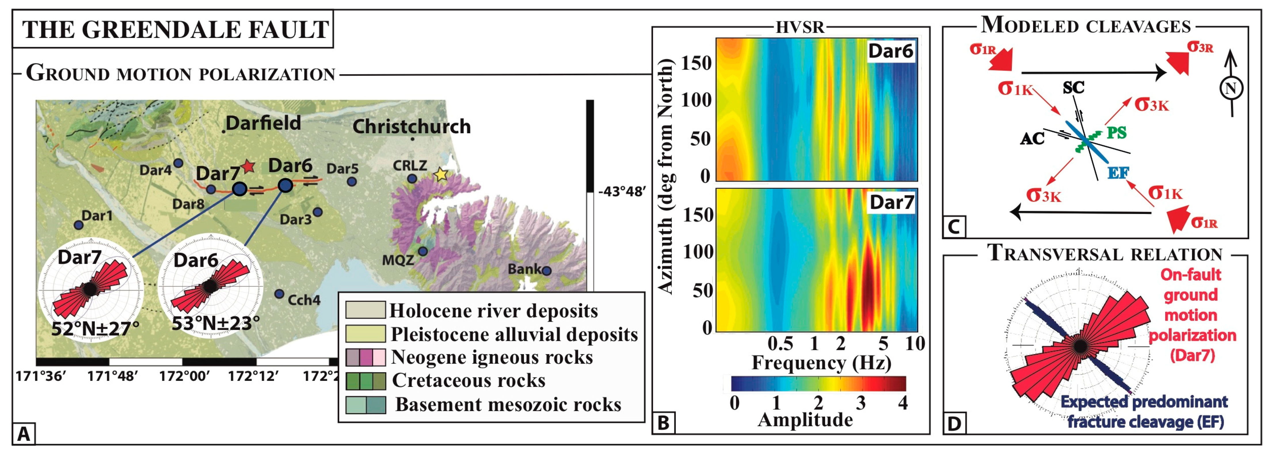
3.2. The Greendale Fault Case Study

The Greendale Fault (GF) is located near the dextral-transpressional deformation zone associated with the oblique collision of the Pacific plate with the Australian plate in New Zealand (Figure 3). It was unknown before the 2010–2011 Canterbury earthquake sequence, beginning in September 2010 with the Darfield Mw 7.1 earthquake (the epicenter identified by a red star in Figure 3A), and the following Mw 6.2 in February of 2011. This latter occurred beneath the city of Christchurch and caused high damage throughout the city due to extensive soil liquefaction (its epicenter is identified by a yellow star in Figure 3A). This complex right-lateral strike-slip fault system was described as “immature”, according to the aftershock distribution [60,61,62,63]. Field and geomorphic evidences are hidden by the Holocene river gravels composing many overlapping fans of glacier rivers descending from the Southern Alps (Figure 3A) that fill the 160 km-long and 50 km-wide Canterbury Plains ([64,65,66] and references therein), reaching a thickness of 1.5 km.
The wavefield polarization was recently determined across the GF using earthquake data recorded by an array of 14 stations installed by the Victoria University of Wellington, together with the University of Auckland and the University of Wisconsin-Madison [34]. The majority of these stations were installed on the flat Canterbury Plains [67,68]. In Figure 3 we show the geological map, modified after [65]. This array recorded thousands of aftershocks following the Darfield earthquake, and occurred from 8 September 2010 to 13 January 2011 [69]. In order to check the result stability independently of the seismic source and path, [34] selected four clusters (Cl-2, Cl-4, Cl41, Cl-54) among the data set prepared by [70] and comprising 163 earthquake magnitudes between 1.8 and 4.8. They assessed the polarization both in the frequency and time domains through the individual-station using HVSRs and covariance matrix analysis (see Section 2), respectively. In addition to earthquake records, they also used ambient noise continuously recorded for 72-days from 19 September 2010.
Pischiutta [34] found that stations installed in the Canterbury Plains have an amplification peak between 0.1 and 0.3 Hz for both earthquakes and ambient noise. The HVSRs reported in Figure 3B were calculated using earthquake signals at stations Dar6 and Dar7. They clearly show the existence of such a low-frequency peak, with amplitudes up to a factor of three, that is related to the resonance of a considerable thickness (c. 1 km) of soft sediments lying over the metamorphic bedrock. The analysis performed using seismic events revealed the existence of another peak in amplification between 2 and 5 Hz at two on-fault stations, which was not visible in the noise analysis. In contrast to the lower frequency peak, the ones between 2 and 5 Hz are more strongly anisotropic, attaining amplitudes up to a factor of four in the N50–60° direction. The covariance matrix analysis led to better identification of the ground motion polarization direction. The two stations installed on the fault, Dar6 and Dar7, show that the narrow rose diagrams peaked in the N52° ± 27° and N53° ± 24° directions, respectively. The results are consistent between the analyzed clusters of seismic events, suggesting that it is not affected by the seismic path, but is rather ascribed to the site subsoil structure. All stations in the Canterbury Plains and at kilometers from the GF (Dar1, Dar2, Dar3, Dar4, Dar5, Cch1, Cch2, Cch4, CRLZ, and MQZ) show very scattered rose diagrams, with no horizontal polarization (see also [34]).
Following the approach described in Section 3, this effect was interpreted in terms of the fracture pattern in the fault damage zone, which was modeled through the package FRAP [34,59]. In Figure 3C we provide a sketch of the right-lateral fault movement in the N90° direction (black arrows), with the regional stress field (red arrows), and the kinematic components of the local stress field (K1 and K3). Modelling showed that extensional fractures are the expected predominant fracture cleavage in the shallow layers (<2 km), with an expected strike of N139° (the blue rose diagram). The fracture orientation is consistent with coseismic surface rupture observations, confirming the reliability of the model. Therefore, the horizontal polarization is orthogonal to the predominant fracture strike (Figure 3D). The ground motion polarization was also compared with the shear-wave anisotropy derived from the shear-wave splitting, confirming such inferences. The relationship between seismic anisotropy ground motion polarization will be discussed later on, in Section 4.

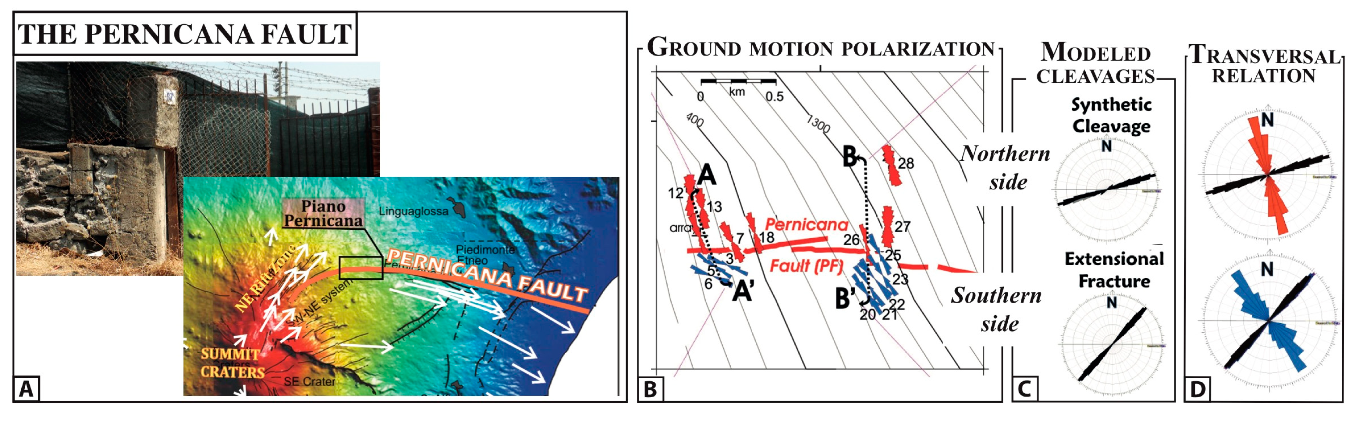
3.3. The Pernicana Fault Case Study

The Pernicana Fault (PF) is the most relevant tectonic lineament of the Mt Etna volcano, located on the Ionian coast of Sicily. The fault extends for a total length of 18 km, from the NE Rift to the coastline [71]. At elevations between 950 and 1530 m, the fault morphology is represented by a scarp (up to 80 m high); the lack of a clear morphological signature in the other zones has been related to the most recent lava cover [72]. Fault activity (slip rates at a centennial scale ranging from 1 to 2.7 cm/yr) results in continuous damage to man-made structures (see Figure 4A) [73,74]. The fault displacement varies from pure left-lateral (to the eastern side near the coastline) to trans tensional (near the intersection with the NE rift, on the Mt Etna summit area). The fault movement is mainly accommodated through creeping [72], but large slip episodes also occurred during shallow (<3 km) earthquakes [74]. The top picture in panel A (taken in 2013) shows visible damage produced by the continuous fault movement to man-made structures.
The PF also represents the northern boundary of a large sliding movement of the E and SE sectors of the volcano [75,76]. The sliding movement occurs towards E to ESE, as indicated by the white arrows in Figure 4A [77,78]. The relation between the flank sliding and the PF is highlighted by the relative downthrow of the S sector prevailing over the movement of the fault.
Figure 4. The Pernicana fault, at Piano Pernicana, Mt. Etna (Italy), redrawn after [79]. (A) Map of the PF [77]. White arrows indicate the horizontal displacement vectors as measured by [77] between 2005 and 2006. The top picture (taken in 2013) shows visible damage produced by the continuous fault movement to man-made structures. (B) Ground motion polarization of each station obtained through the covariance matrix analysis, represented by rose diagrams (in red and blue to the north and south of the fault, respectively). (C) Fracture cleavages in the two sides of the PF fault, modeled by using the FRAP package [59]. (D) Comparison between fracture strike (black rose diagrams) modelled for the two sides of the fault and the horizontal polarization (red and blue rose diagrams to the north and south of the fault, respectively), highlighting a transversal relationship in the two sides of the PF.
Applsci 13 06060 g004
The directional amplification at Piano Pernicana was investigated by [5] using ambient noise measurements and local earthquakes. The main results of their paper are redrawn in Figure 4B. They found variations across the PF damage zone, with an abrupt rotation of the azimuth by about 30° across the fault, varying from N166° to N139° from the northern to the southern fault side on the south (Figure 4B). Such variations in ground motion polarization between the two sides of the fault were interpreted in terms of different deformation and kinematic conditions, resulting in different fracture patterns. A combined numeric and analytic approach was applied using the FRAP Package [59] to determine the most likely expected cleavage on the two sides of the PF (synthetic cleavages, antithetic cleavages, or extensional fractures), as well as their orientations. The two sides of the fault at Piano Pernicana were separately modeled: in the northern side of the PF the left-lateral strike-slip movement prevails, whereas the southern side is also subjected to sliding, and there is a dominant extensional stress regime. Therefore, while in the former the synthetic cleavages predominate, with an overall N74° trend, in the latter the extensional fractures are more diffuse, with an overall N42° trend. They both show a near-orthogonal relation (∼88° in the northern sector and ∼83° to the south) with the azimuth of the observed directional resonance (Figure 4C).
Therefore, as in previous sections, even [79] concluded that the direction of the largest resonance motions is sensitive to and has a transversal relationship with the dominant fracture orientation (Figure 4D).
We finally stress that such findings were recently confirmed by a controlled-source seismic experiment undertaken in the same area to investigate the subsoil capability in generating polarized motion [35]. This study suggested that the propagation of surface waves is more efficient along the observed main polarization direction. In fact, when the shear excitation is orthogonal to the pre- dominant site polarization, ground excitation lost its initial polarization less than 50 m away from the source position.

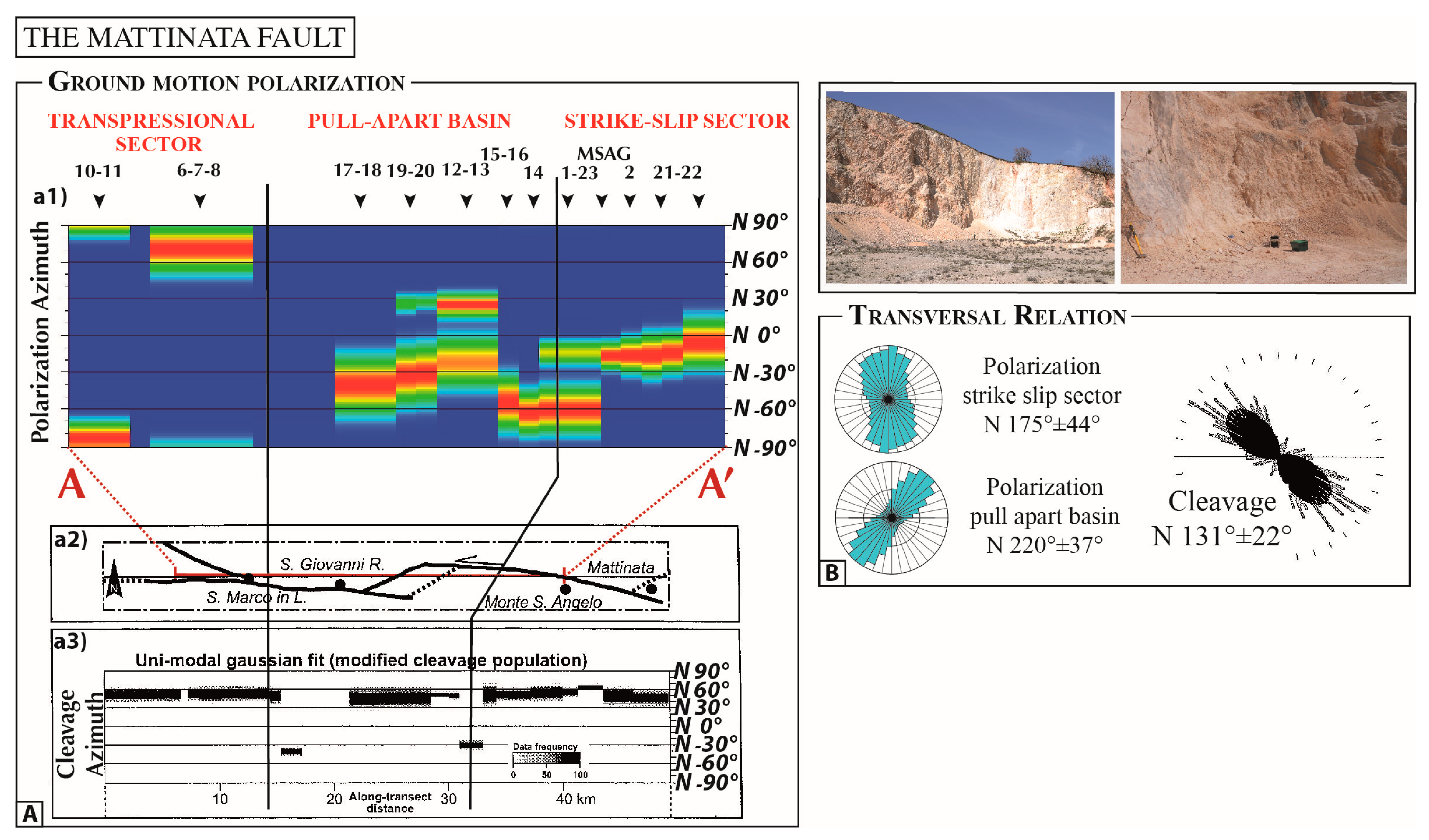
3.4. The Mattinata Fault Case Study

The seismically-active Mattinata fault (MF) outcrops for over 40 km in the Gargano Promontory, Puglia region of southern Italy. It shows an undulated trajectory that is characterized by a number of significant tectonic-related morphological features, compatible with general, long-lasting, left-lateral strike-slip kinematics, although a present-day right-lateral activity has been detected by the focal mechanism solution of an earthquake along this fault [80]. These features include a pull-apart basin and a transpressional zone. In Figure S1, we redraw the geological map of MF given in [59], marking the pull apart basin and transpressional sector in yellow and blue, respectively. The authors analyzed the cleavage sets of the MF and established a number of geometrical and kinematic relationships between the fault and the associated cleavage system. They found that the main associated cleavage consists of a marked array of disjunctive, spaced pressure-solution surfaces developed within the 200–300 m wide fault damage zone that is bounded by unfractured wall rocks. The cleavage-fault angle is almost constantly equal to 40°. It slightly increases in the pull-apart basins and decreases in the transpessional segment.
Considering the high number of structural investigations performed in the above cited study, this fault was chosen to apply the study of wavefield polarization using ambient noise records [81]. Ambient vibrations were recorded at about 30 sites chosen (at a duration between 20 and 50 min) in the fault damage zone, close to available structural geological measurements at rock outcrops. The stations were equipped with a high-dynamic seismic digitizer (Reftek 130) and a three-component sensor with an eigenperiod of 5 s (Lennartz LE-5s). All measurements were performed according to SESAME (Site EffectS assessment using Ambient Excitations http://sesame.geopsy.org/SES_Home_Description.htm, last accessed 16 April 2023) guidelines. The tendency of ground motion to be polarized in the horizontal plane was evaluated in the frequency domain through rotated HVSR (see Section 1) using Geopsy software [82] (http://www.geopsy.org, last accessed on 19 April 2023), after applying an anti-trigger algorithm, to select the most stationary part of the signals [82]. The results are given as rose diagrams in Figure S1 for some exemplificative sites. In Figure S2, we also show the contour plots of the HVSR amplitudes. An ambient noise measurement was performed close to the permanent broadband station of the Italian Seismic Network MSAG. The HVSR obtained on ambient noise (Figure S2) were found to be consistent with those inferred on earthquake records [83], both in terms of the amplified frequency band (broadband from 2 to 8 Hz) and in terms of the direction of maximum amplification (roughly NNE-SSW). This confirmed that ambient noise yields a result consistent with earthquake records, as observed in many other previous studies [5,25]. In the time domain, the covariance matrix analysis was applied at each station’s noise signals (see Section 2), after bandpass filtering signals in the amplified frequency band (as suggested by the HVSR results). The rose diagrams shown Figure S1 were obtained by using all values of polarization azimuths at each station, even adding the results from groups of nearby stations.
In Figure 5A, the variation of polarization across the fault is plotted along the transect AA′ using the transect diagrams computed with the package Daisy, and is compared with the measured pressure solution cleavage in [59]. In spite of the high complexity of results, the observed pattern is not random, and there is a general tendency of polarization to be oriented transverse to the outcropping pressure-solution cleavage (Figure 5B). In the sectors where the MF exhibits a pure strike-slip kinematics and in the pull-apart region, the majority of the polarization measurements show polarization transverse to the fault-related cleavages. There are some sites where a different polarization occurs, which may be associated to a corresponding orthogonal cleavage. In the transpressional sector of the fault, it seems that the relationship between the polarization and the cleavages is more complex, probably due to the complexity of deformation in transtensional fault regimes, often preventing them from the development of the regionally homogeneous fracture sets which are required to produce ground motion polarization on a wide scale.
Another possibility is that the Mattinata Fault acts as a transfer fault, with its relative motion varying or even inverting, depending on the relative motion between the Northern and the Southern blocks that it separates.
With the exception of the transpressional zone, the analyses on the MF confirm the existence of a high angle (orthogonal) relationship between the ground motion polarization and fractures and the proposed model (Figure 5B).

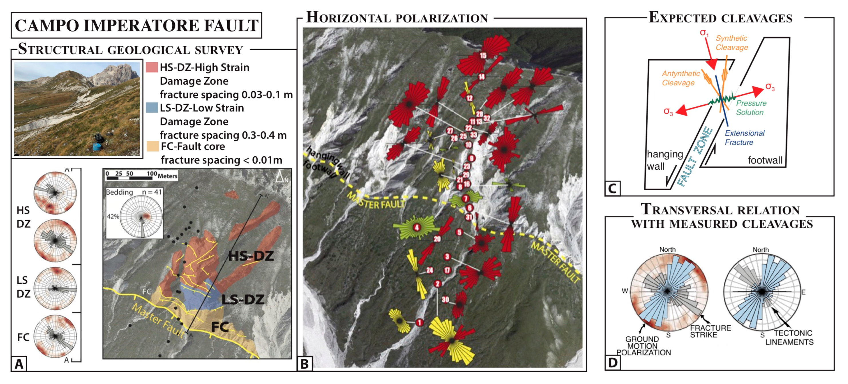
3.5. The Campo Imperatore Fault Case Study

A similar study was led out by [26], who assessed the ambient noise amplification across the Vado di Corno Fault (VCF, Campo Imperatore, central Italy, where a very detailed structural geological survey was recently led out [84], revealing the high anisotropy of the fault that is affected by a complex network of faults and fractures with a dominant WNW–ESE strike. A summary of their results is redrawn in Figure 6A. In the same area, Ref. [26] measured seismic noise along a ∼500 m long transect perpendicular to the average fault strike. Ambient noise signals were processed using the covariance matrix analysis (see Section 1). Rose diagrams from the covariance matrix analysis are given in Figure 6B, their dimension being scaled according to the HVSR amplitude peak. They provide the mean direction of motion horizontal polarization at each station. The results were grouped in three classes on the basis of the dominant horizontal polarization: NNW–SSE (yellow rose diagrams); NE–SW fault-transverse (red rose diagrams); E–W (green rose diagrams). The majority of the recordings showed a predominant NNE–SSW to NE–SW amplification of the horizontal component of the seismic waves, transverse to the average strike of the fault-fracture network.
Seismic signals were also processed calculating the HVSRs and using the time frequency polarization analyses. The results at four representative stations are given in Figure S3 (CAM6, CAM11, CAM15, CAM24). The HVSR calculated using the Geopsy software show a resonance peak at about 1 Hz, with amplitudes over a factor of 5, and ground motion amplification occurring along the azimuth N20°, according to ground motion polarization assessed through a covariance matrix analysis. The direction of maximum amplification varies to N160° at station CAM24. The results by time– frequency (TF) polarization analysis (see Section 2) show consistent results, with the ellipticity plot vs frequency showing minimum values at frequency ranges corresponding to the amplification at HVSR, giving an indication of the linear polarization. Moreover, the strike polar plot indicates polarization at the azimuth compatible with the HVSR and covariance matrix analyses.
Finally, numerical simulations of earthquake ground motions in [26] ruled out the possibility that the observed effect is produced by the topographic irregularity, confirming that the higher amplitudes of ambient noise observed in the fault-perpendicular direction were due to a site effect (i.e., the fracture network and the resulting stiffness anisotropy of the rock mass).

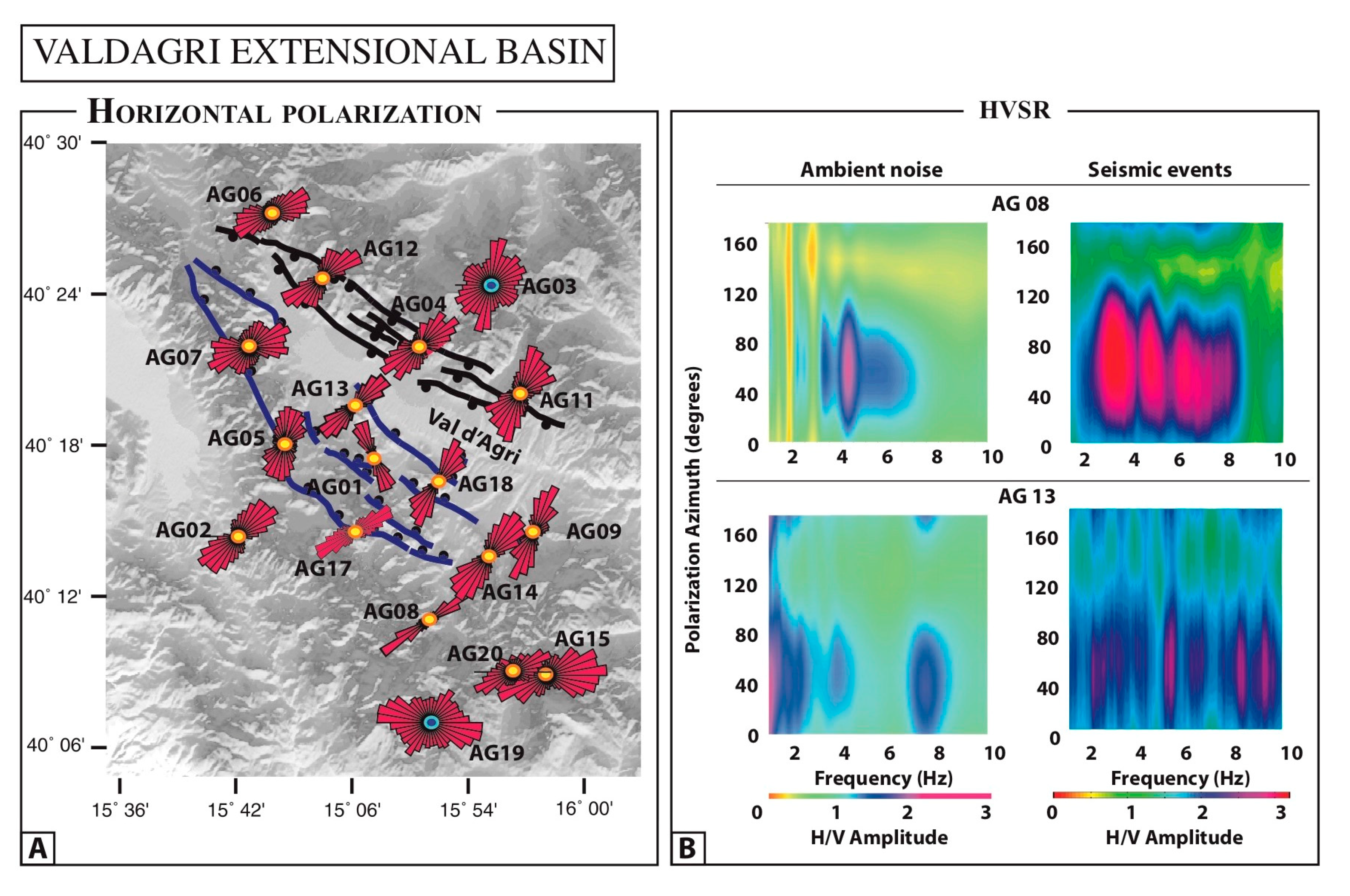
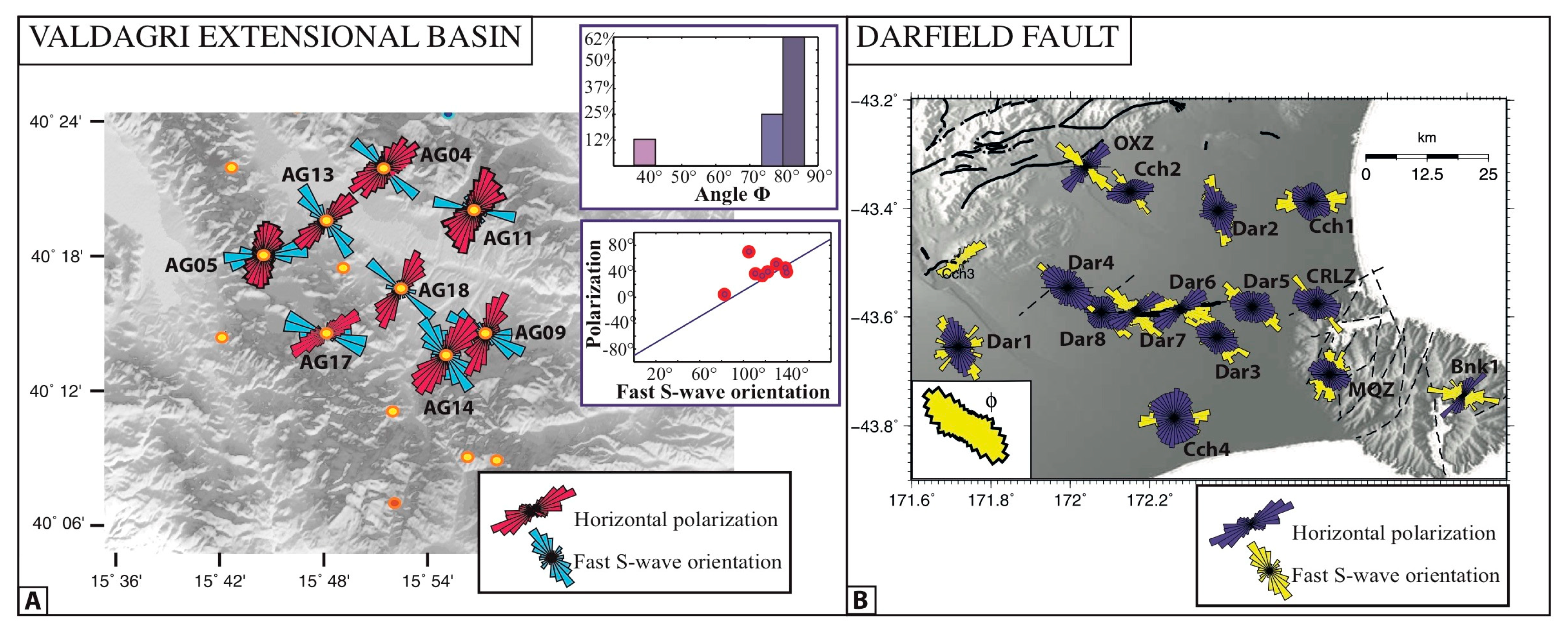
3.6. The Val d’Agri Case Study

Conversely to the effect of trapped waves, which are spatially limited to small fault sections (e.g., [9,85]), ground motion directional amplification and polarization due to fractures can involve larger extensions. As an example, in the Val d’Agri sector [34] found that such effects are consistently observed in a several kilometre-wide areas. The Val d’Agri area hosts the largest oil fields of the southern Apennines, whose high productivity was related to the presence of open and permeable fracture networks held open by the tectonic stress. Here, a 30-km wide Quaternary graben basin was filled by up to 500 m of continental deposits, and is bordered by two systems of NW-SE trending, high- angle normal faults: (i) the Eastern Agri fault system (EAFS), with subparallel SW dipping strands and a vertical displacement of ~500 m; and (ii) the NE dipping Monti della Maddalena fault system (MMFS in [86]), which is the main structure accommodating the active extension in the area. In Figure 7A, they are represented with black and blue lines, respectively. They are both consistent with the local active stress field inferred borehole breakout, seismological, and hydrocarbon production data.
In this area, wavefield polarization was investigated using a network of 20 stations installed on a rock outcrop (yellow dots in Figure 7A) using signals by almost 200 seismograms (the database was created by [87,88]). We redrew [33] the findings in terms of rose diagrams representing ground motion polarization (Figure 7A). They are obtained by merging all of the analyzed seismic events at each station. At most stations a persistent horizontal polarization is observed along the NE-SW direction, transverse to the general trend of Quaternary normal faults and to the maximum horizontal stress related to the present extensional regime. This amplification effect is confirmed by HVSR calculated at stations AG08 and AG13 by using confirmed seismic events and ambient noise (Figure 7B). In fact, as evidenced by the high number of data from hydrocarbon exploration and production, in this sector the acting local stress regime has a primary role in opening cracks and fractures which strike NW-SE, parallel to the SHmax direction, which are open and saturated by fluids (water and oil). Conversely, cracks and fractures with an orthogonal strike tend to be closed (Trice, 1999).

4. The Transversal Relation between Ground Motion Polarization and Velocity Anisotropy

As illustrated in previous sections, directional horizontal motions can occur in fault zones as the effect of the larger compliance transversal to fractures in the fault damage zone. Moreover, in fault zones, the fast S wave direction is controlled by the crack orientation (rather than the regional stress) [69,89,90,91].
The comparison between horizontal polarization and S wave fast direction was led out, up to now, in three papers [23,33,34]. Since these two parameters are estimated in a completely different approach, and considering the different portions of seismograms, it represents a useful test of consistency.
In the Val d’Agri region, Refs. [91,92] found an S wave fast direction perpendicular to the current regional extension, as the effect of open and fluid-saturated cracks in fractured carbonate rocks aligned by the active stress field. Pischiutta et al. in [33] recognized a transverse relation between horizontal polarization (red rose diagram) and fast S wave direction (cyan rose diagrams), as shown in Figure 8A. Therefore, open and fluid-saturated cracks affect both (i) the velocity anisotropy of seismic waves (they travel faster parallel to fractures), and (ii) the ground motion horizontal polarization (due to the higher compliancy in the direction orthogonal to the fractures).
Similar findings were observed in the GF, a newly fractured strike-slip fault system [33]. In Figure 8B, we show the comparison between ground motion polarization (yellow rose diagrams) and fast S-wave orientation (yellow rose diagrams), as assessed by [34,70].
Furthermore [23] investigated the seismic wavefield polarization within a transform zone in the Reykjanes Peninsula volcanic rift zone (south Iceland), finding that ground motion polarization has a perpendicular relationship with mapped faults and fractures, as well with fast S wave directions.
This suggested that wavefield polarization and fast velocity direction are effects of the same cause: an anisotropic medium (fractured rocks) where Vs is larger in the crack-parallel component (causing seismic anisotropy) and compliance is larger perpendicular to the crack strike (causing horizontal ground motion).

5. Final Remarks

Much effort has been devoted in recent decades to the study of peculiar directional amplification effects across fault zones. In this paper, we discussed our main findings at several fault zones, characterized by different geological settings and kinematics. The common feature of all case studies is the occurrence of DA and ground motion polarization perpendicular to the predominant fracture field. These latter findings were defined through both the modelling of the fracture pattern in the fault damage zone (package FRAP [59]), and the detailed structural surveys. Such an orthogonal relation between ground motion polarization and fractures was also confirmed by a comparison with the results of an S-wave splitting analysis, which was used as a proxy to define the orientation of open fractures at a larger depth [23,33,34].
DA and polarization effects orthogonal to fractures completely differ from fault-zone trapped waves, with the latter showing polarization oriented parallel to the fault strike. Moreover, while the effect of trapped waves is spatially limited to small fault sections (e.g., [9,85], ground motion DA and polarization due to fractures can involve relevant areal extents up to several kilometers wide, as suggested by the Val d’Agri case study (see also [33]).
The site-effects produced by the presence of fractures at rock sites can have significant implications. First, the existence of amplification effects at rock sites can raise relevant implications both in terms of seismic hazard and in engineering applications, as in GMPEs (ground motion prediction equations) exploitation, where they are considered to be free from resonance and amplification effects (e.g., [93,94]), and in ground motion simulation techniques made for ground motion prediction purposes. The current state of knowledge is limited to the relative amplification between horizontal and vertical components, and further estimates are needed to evaluate absolute amplitude and to understand to what extent this effect could be important for seismic hazard and engineering applications. Another implication involves the choice of a reference site for site-response estimates, as, for example, in the standard spectral ratio method [36]. Several authors have already stressed how rock sites can have their own site response, an arbitrary choice of a reference rock site leading to a bias on the estimates of the site effect (e.g., [95,96,97,98]). Lanzano in [94] highlighted that the amplification effects at rock sites have an influence on the prediction of the expected motion among the recording stations of the Italian Accelerometric Archive (ITACA, http://itaca.mi.ingv.it, last accessed on 16 April 2023, [99]).
Finally, rock sites are also considered to be preferred locations for permanent seismic stations, where the occurrence of DA may lead to higher amplitude levels and to incorrect earthquake magnitude estimates. Recent papers involving stations of permanent networks have highlighted that the DA effects can involve a high number of rock sites among stations of permanent seismic networks [83,100,101].

Supplementary Materials

The following supporting information can be downloaded at: https://www.mdpi.com/article/10.3390/app13106060/s1. Table S1—Data selection used in the Hayward fault, downloaded through the IRIS Wilber3 tool (http://ds.iris.edu, last accessed on 19 April 2021): hypocentral parameters and station record. Figure S1—The Mattinata fault, Gargano Promontory (Puglia, southern Italy). The geological map of MF given in Salvini et al. ii (1999), marking the pull apart basin and transpressional sector in yellow and blue, respectively. The top picture shows some sectors of the fault, with pervasive fracturing. The location of ambient noise measurements is shown as well, together with rose diagrams representing horizontal ground motion polarization obtained through the covariance matrix analysis. They were obtained by using all values of polarization azimuths at each station, even adding the results from groups of nearby stations. Figure S2—HVSR results given for some exemplificative sites. To visualize the variation versus azimuth, HVSR single curves are shown for each rotation step. Moreover, contour plots of the HVSR amplitudes are shown as a function of frequency (x-axis) and angle of rotation (y-axis). Figure S3—The Campo Imperatore fault, Abruzzi (central Italy). Left-panel: HVSR at four selected stations (CAM6, CAM11, CAM15, CAM24) calculated using Geopsy software (Wathelet, 2005). Right panel: Results by time–frequency (TF) polarization analysis. An ellipticity plot vs. frequency shows minimum values at frequency ranges corresponding to amplification at HVSR, giving an indication of the linear polarization. Moreover, the strike polar plot indicates polarization at the azimuth compatible with HVSR and covariance matrix analyses.

Author Contributions

Conceptualization, M.P. and A.R.; methodology, M.P., A.R., F.S., J.B.F. and M.K.S.; formal analysis, M.P.; investigation, M.P., A.R., F.S., J.B.F. and M.K.S.; data curation, M.P., J.B.F. and M.K.S.; writing—original draft preparation, review, editing, M.P., A.R., F.S., J.B.F. and M.K.S. All authors have read and agreed to the published version of the manuscript.

Funding

This research received no external funding.

Institutional Review Board Statement

Not applicable.

Informed Consent Statement

Not applicable.

Data Availability Statement

The earthquake data across the Hayward fault that were analyzed in this study are openly available in http://ds.iris.edu, last accessed on 19 April 2021 The earthquake data used across the Greendale fault are available in the Victoria University of Wellington data system, the GeoNet system, and the IRIS data center. The other data presented in this study are available on request from the corresponding author. They are not publicly available because a public archive was not created.

Acknowledgments

In this work we resume our pursuit of knowledge about directional amplification across fault zones that began in the last decade since the PhD thesis of MP. We thank all coauthors who contributed to the cited papers for their assistance: Larry Baker, Russel Sell, Christopher Dietel, Maurizio Vassallo, Giuseppe Di Giulio, Fabrizio Cara, Michele Fondriest, Matteo Demurtas, Giulio di Toro, Mario Anselmi, and Paola Cianfarra. For useful and important early discussion about the observed effects, we are indebted to John Haines, Yehuda Ben Zion, Paul Spudich, Dave Boore, and Luigi Improta.

Conflicts of Interest

The authors declare that they have no conflict of interest.

References

  1. Bonamassa, O.; Vidale, J.E. Directional site resonances observed from aftershocks of the 18 October Loma Prieta earthquake. Bull. Seism. Soc. Am. 1991, 81, 1945–1957. [Google Scholar]
  2. Lombardo, G.; Rigano, R. Amplification of ground motion in fault and fracture zones: Observations from the Tremestieri fault, Mt. Etna (Italy). J. Volc. Geoth. Res. 2006, 153, 167–176. [Google Scholar] [CrossRef]
  3. Martino, S.; Minutolo, A.; Paciello, A.; Rovelli, A.; Scarascia Mugnozza, G.; Verubbi, V. Evidence of Amplification Effects in Fault Zone Related to Rock Mass Jointing. Nat Hazards 2006, 39, 419–449. [Google Scholar] [CrossRef]
  4. Rigano, R.; Cara, F.; Lombardo, G.; Rovelli, A. Evidence of ground motion polarization on fault zones of Mount Etna volcano. J. Geophys. Res. 2008, 113. [Google Scholar] [CrossRef]
  5. Di Giulio, G.; Cara, F.; Rovelli, A.; Lombardo, G.; Rigano, R. Evidences for strong directional resonances in intensely deformed zones of the Pernicana fault, Mount Etna, Italy. J. Geophys. Res. 2009, 114. [Google Scholar] [CrossRef]
  6. Falsaperla, S.; Cara, F.; Rovelli, A.; Neri, M.; Behncke, B.; Acocella, V. Effects of the 1989 fracture system in the dynamics of the upper SE flank of Etna revealed by volcanic tremor data: The missing link? J. Geophys. Res. 2010, 115. [Google Scholar] [CrossRef]
  7. Ben-Zion, Y.; Aki, K. Seismic radiation from an SH line source in a laterally heterogeneous planar fault zone. Bull. Seism. Soc. Am. 1990, 80, 971–994. [Google Scholar] [CrossRef]
  8. Li, Y.L.; Ellsworth, G.W.; Thurber, C.H.; Malin, P.E.; Aki, K. Observations of fault zone trapped waves excited by explosions at the San Andreas fault, central California. Bull. Seism. Soc. Am. 1997, 87, 210–221. [Google Scholar] [CrossRef]
  9. Lewis, M.A.; Peng, Z.; Ben-Zion, Y.; Vernon, F.L. Shallow seismic trapping structure in the San Jacinto fault zone near Anza, California. Geophys. J. Int. 2005, 162, 867–881. [Google Scholar] [CrossRef]
  10. Mizuno, T.; Nishigami, K. Deep structure of the Mozumi-Sukenobu fault, central Japan, estimated from the subsurface array observation of fault zone trapped waves. Geophys. J. Int. 2006, 159, 622–642. [Google Scholar] [CrossRef]
  11. Spudich, P.; Olsen, K.B. Fault zone amplified waves as a possible seismic hazard along the Calaveras Fault in central California. Geophys. Res. Lett. 2001, 28, 2533–2536. [Google Scholar] [CrossRef]
  12. Calderoni, G.; Rovelli, A.; Di Giovambattista, R. Large amplitude variations recorded by an on-fault seismological station during the L’Aquila earthquakes: Evidence for a complex fault-induced site effect. Geophys. Res. Lett. 2010, 37, L24305. [Google Scholar] [CrossRef]
  13. Cultrera, G.; Rovelli, A.; Mele, G.; Azzara, R.; Caserta, A.; Marra, F. Azimuth dependent amplification of weak and strong ground motions within a fault zone, Nocera Umbra, Central Italy. J. Geophys. Res. 2003, 108, 2156–2170. [Google Scholar] [CrossRef]
  14. Peng, Z.; Ben-Zion, Y. Systematic analysis of crustal anisotropy along the Karadere Duzce branch of the North Anatolian fault. Geophys. J. Int. 2006, 159, 253–274. [Google Scholar] [CrossRef]
  15. Karabulut, H.; Bouchon, M. Spatial variability and non-linearity of strong ground motion near a fault. Geophys. J. Int. 2007, 170, 262–274. [Google Scholar] [CrossRef]
  16. Pischiutta, M. The Polarization of Horizontal Ground Motion: An Analysis of Possible Causes. Ph.D. Thesis, University of Bologna, Italy, 2010; 172p. Available online: http://amsdottorato.unibo.it/3106/ (accessed on 1 July 2022).
  17. Pischiutta, M.; Salvini, F.; Fletcher, J.; Rovelli, A.; Ben-Zion, Y. Horizontal polarization of ground motion in the Hayward fault zone at Fremont, California: Dominant fault-high-angle polarization and fault- induced cracks. Geophys. J. Int. 2012, 188, 1255–1272. [Google Scholar] [CrossRef]
  18. Di Giulio, G.; Amoroso, S.; Di Naccio, D.; Falcucci, E.; Gori, S.; Hailemikael, S.; Vassallo, M.; Ciampaglia, A.; De Luca, G.; Del Grosso, A.; et al. The Seismic Microzonation of San Gregorio Through a Multidisciplinary Approach. Seismic Amplification in a Stiff Site. In Engineering Geology for Society and Territory; Springer: Cham, Switzerland, 2005; Volume 5. [Google Scholar] [CrossRef]
  19. Di Naccio, D.; Vassallo, M.; Di Giulio, G.; Amoroso, S.; Cantore, L.; Hailemikael, S.; Falcucci, E.; Gori, S.; Milana, G. Seismic amplification in a fractured rock site. The case study of San Gregorio (L’Aquila, Italy). Phys. Chem. Earth 2017, 98, 90–106. [Google Scholar] [CrossRef]
  20. Hailemikael, S.; Lenti, L.; Martino, S.; Paciello, A.; Rossi, D.; Scarascia Mugnozza, G. Ground-motion amplification at the Colle di Roio ridge, central Italy: A combined effect of stratigraphy and topography. Geophys. J. Int. 2016, 206, 1–18. [Google Scholar] [CrossRef]
  21. Marzorati, S.; Ladina, C.; Falcucci, E.; Gori, S.; Saroli, M.; Ameri, G.; Galadini, F. Site effects “On the Rock”: The case study of Castelvecchio Subequo (L’Aquila, central Italy). Bull. Earthq. Eng. 2011, 9, 841–868. [Google Scholar] [CrossRef]
  22. Panzera, F.; Tortorici, G.; Romagnoli, G.; Marletta, G.; Catalano, S. Empirical evidence of orthogonal relationship between directional site effects and fracture azimuths in an active fault zone: The case of the Mt. Etna lower eastern flank. Eng. Geol. 2020, 279, 105900. [Google Scholar] [CrossRef]
  23. Panzera, F.; Halldorsson, B.; Vogfjord, K. Directional effects of tectonic fractures on ground motion site amplification from earthquake and ambient noise data: A case study in South Iceland. Soil Dyn. Earthq. Eng. 2017, 97, 143–154. [Google Scholar] [CrossRef]
  24. Panzera, F.; D’Amico, S.; Colica, E.; Viccaro, M. Ambient vibration measurements to support morphometric analysis of a pyroclastic cone. Bull. Volcanol. 2019, 81, 74. [Google Scholar] [CrossRef]
  25. Panzera, F.; Pischiutta, M.; Lombardo, G.; Monaco, C.; Rovelli, A. Wavefield Polarization in Fault Zones of the Western Flank of Mt. Etna: Observations and Fracture Orientation Modelling. Pure Appl. Geophys. 2014, 171, 3083–3097. [Google Scholar] [CrossRef]
  26. Pischiutta, M.; Fondriest, M.; Demurtas, M.; Magnoni, F.; Di Toro, G.; Rovelli, A. Structural control on the directional amplification of seismic noise (Campo Imperatore, central Italy). Earth Planet. Sci. Lett. 2017, 471, 10–18. [Google Scholar] [CrossRef]
  27. Burjanek, J.; Moore, J.R.; Yugsi Molina, F.X.; Faeh, D. Instrumental evidence of normal mode rock slope vibration. Geophys. J. Int. 2012, 188, 559–569. [Google Scholar] [CrossRef]
  28. Burjanek, J.; Gassner-Stamm, G.; Poggi, V.; Moore, J.R.; Fah, D. Ambient vibration analysis of an unstable mountain slope. Geophys. J. Int. 2010, 180, 820–828. [Google Scholar] [CrossRef]
  29. Del Gaudio, V.; Wasowski, J. Directivity of slope dynamic response to seismic shaking. Geophys. Res. Lett. 2007, 34, L12301. [Google Scholar] [CrossRef]
  30. Del Gaudio, V.; Wasowski, J.; Muscillo, S. New developments in ambient noise analysis to characterise the seismic response of landslide-prone slopes. Nat. Hazards Earth Syst. Sci. 2013, 13, 2075–2087. [Google Scholar] [CrossRef]
  31. Moore, J.; Gischig, V.; Burjanek, J.; Loew, S.; Faeh, D. Site effects in unstable rock slopes: Dynamic behavior of the Randa instability (Switzerland). Bull. Seism. Soc. Am. 2011, 101, 3110–3116. [Google Scholar] [CrossRef]
  32. Moore, J.R.; Geimer, P.R.; Finnegan, R.; Thorne, M.S. Use of Seismic Resonance Measurements to Determine the Elastic Modulus of Freestanding Rock Masses. Rock Mech. Rock Eng. 2008, 51, 3937–3944. [Google Scholar] [CrossRef]
  33. Pischiutta, M.; Pastori, M.; Improta, L.; Salvini, F.; Rovelli, A. Orthogonal relation between wavefield polarization and fast S-wave direction in the Val d’Agri region: An integrating method to investigate rock anisotropy. J. Geophys. Res. Solid Earth 2014, 119, 1–13. [Google Scholar] [CrossRef]
  34. Pischiutta, M.; Savage, M.; Holt, R.; Salvini, F. Fracture-related wavefield polarization and seismic anisotropy across the Greendale Fault. J. Geophys. Res. Solid Earth 2015, 120, 7048–7067. [Google Scholar] [CrossRef]
  35. Di Giulio, G.; Punzo, M.; Bruno, P.P.; Cara, F.; Rovelli, A. Using a vibratory source at Mt. Etna (Italy) to investigate the wavefield polarization at Pernicana Fault. Near Surf. Geophys. 2019, 17, 313–329. [Google Scholar] [CrossRef]
  36. Borcherdt, R.D. Effects of local geology on ground motion near San Francisco Bay. Bull. Seism. Soc. Am. 1970, 60, 29–61. [Google Scholar]
  37. Tucker, B.E.; King, J.L.; Hatzfeld, D.; Nersesov, I.L. Observations of hard-rock site effects. Bull. Seim. Soc. Am. 1987, 74, 121–136. [Google Scholar] [CrossRef]
  38. Lermo, J.; Chavez-Garcia, F.J. Site effect evaluation using spectral ratios with only one station. Bull. Seismol. Soc. Am. 1993, 83, 1574–1594. [Google Scholar] [CrossRef]
  39. Field, E.H.; Jacob, K.H. A comparison and test of various site response estimation techniques, including three that are not reference site dependent. Bull. Seism. Soc. Am. 1995, 85, 1127–1143. [Google Scholar]
  40. Faeh, D.; Kind, F.; Giardini, D. A theoretical investigation of average H/V ratios. Geophys. J. Int. 2001, 145, 535–549. [Google Scholar] [CrossRef]
  41. Guo, Z.; Aydin, A. A modified HVSR method to evaluate site effect in Northern Mississippi considering ocean wave climate. Eng. Geol. 2016, 200, 104–113. [Google Scholar] [CrossRef]
  42. Guo, Z.; Xue, M.; Aydin, A.; Huang, Y. Locating the Source Regions of the Single and Double-Frequency Microseisms to Investigate the Source Effects on HVSR in Site Effect Analysis. J. Earth Sci. 2022, 33, 1219–1232. [Google Scholar] [CrossRef]
  43. Spudich, P.; Hellweg, M.; Lee, W.H.K. Directional topographic site response at Tarzana observed in aftershocks of the 1994 Northridge, California, earthquake: Implications for mainshock motions. Bull. Seismol. Soc. Am. 1996, 86, S193–S208. [Google Scholar] [CrossRef]
  44. Konno, K.; Ohmachi, T. Ground-motion characteristics estimated from spectral ratio between horizontal and vertical components of microtremor. Bull. Seismol. Soc. Am. 1998, 88, 228–241. [Google Scholar] [CrossRef]
  45. Kanasewich, E.R. Time Sequence Analysis in Geophysics; University of Alberta Press: Edmonton, AB, Canada, 1980; 477p. [Google Scholar]
  46. Jurkevics, A. Polarization analysis of three component array data. Bull. Seismol. Soc. Am. 1988, 78, 1725–1743. [Google Scholar]
  47. La Rocca, M.; Galluzzo, D.; Saccorotti, G.; Tinti, S.; Cimini, G.B.; Del Pezzo, E. Seismic signals associated with landslides and with a tsunami at Stromboli volcano, Italy. Bull. Seismol. Soc. Am. 2004, 94, 1850–1867. [Google Scholar] [CrossRef]
  48. Napolitano, F.; Gervasi, A.; La Rocca, M.; Guerra, I.; Scarpa, R. Site effects in the Pollino region from spectral and polarization analyses of seismic noise and earthquakes. Bull. Seismol. Soc. Am. 2018, 108, 309–321. [Google Scholar] [CrossRef]
  49. Formisano, L.A.; La Rocca, M.; Del Pezzo, E.; Galluzzo, D.; Fischione, C.; Scarpa, R. Topography effects in the polarization of earthquake signals: A comparison between surface and deep recordings. Boll. Geofis. Teor. Appl. 2012, 53, 471–484. [Google Scholar] [CrossRef]
  50. Vidale, J.E. Complex polarization analysis of particle motion. Bull. Seismol. Soc. Am. 1986, 76, 1393–1405. [Google Scholar]
  51. Pischiutta, M.; Petrosino, S.; Nappi, R. Directional amplification and ground motion polarization in Casamicciola area (Ischia volcanic island) after the 21 August 2017 Md 4.0 earthquake. Front. Earth Sci. 2022, 10, 999222. [Google Scholar] [CrossRef]
  52. Kelson, K.I.; Simpson, G.D. Late Quaternary deformation of the Southern East Bay Hills, Alameda County, California. Am. Assoc. Petrol. Geol. Bull. 1995, 79, 590. [Google Scholar]
  53. Graymer, R.W.; Sarna-Wojcicki, A.M.; Walker, J.P.; McLaughlin, R.J.; Fleck, R.J. Controls on timing and amount of right-lateral offset on the East Bay fault system, San Francisco Bay region, California. Bull. Geol. Soc. Am. 2002, 114, 1471–1479. [Google Scholar] [CrossRef]
  54. Lienkaemper, J.J.; Galehouse, J.S.; Simpson, R.W. Long-term monitoring of creep rate along the Hayward fault and evidence for a lasting creep response to 1989 Loma Prieta earthquake. Geophys. Res. Lett. 2001, 28, 2265–2268. [Google Scholar] [CrossRef]
  55. Savage, J.C.; Lisowski, M. Inferred depth of creep on the Hayward fault, central California. J. Geophys. Res. 1993, 98, 787–793. [Google Scholar] [CrossRef]
  56. Bakun, W.H. Seismic activity of the San Francisco Bay region. Bull. Seismol. Soc. Am. 1999, 89, 764–784. [Google Scholar] [CrossRef]
  57. Yu, E.; Segall, P. Slip in the 1868 Hayward earthquake from the analysis of historical triangulation data. J. Geophys. Res. 1996, 101, 16101–16118. [Google Scholar] [CrossRef]
  58. Spudich, P.; Xu, L. Documentation of software package ISOSYN: Isochrone integration programs for earthquake ground motion calculations. In CD Accompanying IASPEI Handbook of Earthquake & Engineering Seismology; Academic Press: Cambridge, MA, USA, 2003; 72p. [Google Scholar]
  59. Salvini, F.; Billi, A.; Wise, D.U. Strike-slip fault-propagation cleavage in carbonate rocks: The Mattinata Fault Zone, Southern Apennines, Italy. J. Struct. Geol. 1999, 21, 1731–1749. [Google Scholar] [CrossRef]
  60. Beavan, J.; Fielding, E.; Motagh, M.S.; Samsonov, S.; Donnelly, N. Fault location and slip distribution of the 22 February 2011 Mw 6.2 Christchurch, New Zealand, earthquake from geodetic data. Seismol. Res. Lett. 2001, 82, 789–799. [Google Scholar] [CrossRef]
  61. Gledhill, K.; Ristau, J.; Reyners, M.; Fry, B.; Holden, C. The Darfield (Canterbury, New Zealand) Mw 7.1 earthquake of September 2010: A preliminary seismological report. Seismol. Res. Lett. 2001, 82, 379–386. [Google Scholar] [CrossRef]
  62. Syracuse, E.M.; Thurber, C.H.; Rawles, C.J.; Savage, M.K.; Bannister, S. High-resolution relocation of aftershocks of the Mw 7.1 Darfield, New Zealand, earthquake and implications for fault activity. J. Geophys. Res. Solid Earth 2013, 118, 4184–4195. [Google Scholar] [CrossRef]
  63. Kaiser, A.; Holden, C.; Beavan, J.; Beetham, D.; Benites, R.; Celentano, A.; Collett, D.; Cousins, J.; Cubrinovski, M.; Dellow, G.; et al. The Mw 6.2 Christchurch earthquake of February 2011: Preliminary report. N. Z. J. Geol. Geophys. 2012, 55, 67–90. [Google Scholar] [CrossRef]
  64. Van Dissen, R. Surface rupture displacement on the Greendale Fault during the Mw 7.1 Darfield (Canterbury) earthquake, New Zealand, and its impact on man-madestructures. In Proceedings of the Ninth Pacific Conference on Earthquake Engineering: Building an Earthquake-Resilient Society, Auckland, New Zealand, 14–16 April 2011; pp. 186–193. [Google Scholar]
  65. Forsyth, P.J.; Barrell, D.J.A.; Jongens, R. Geology of the Christchurch Area: Institute of Geological and Nuclear Sciences Geological Map, 2008, Map 16 Lower Hutt New Zealand, Scale 1:250,000, 1 Sheet, 67 p. Text. Available online: https://natlib.govt.nz/records/20620551?search%5Bi%5D%5Bsubject%5D=Geology+--+New+Zealand+--+Canterbury&search%5Bpath%5D=items (accessed on 1 July 2022).
  66. Guidotti, R.; Stupazzini, M.; Smerzini, C.; Paolucci, R.; Ramieri, P. Numerical study on the role of basin geometry and kinematic seismic source in 3D ground motion simulation of the 22 February 2011 MW 6.2 Christchurch earthquake. Seismol. Res. Lett. 2011, 82, 767–782. [Google Scholar] [CrossRef]
  67. Ghisetti, F.C.; Sibson, R.H. Compressional reactivation of E–W inherited normal faults in the area of the 2010–2011 Canterbury earthquake sequence, N.Z.J. Geol. Geophys. 2012, 55, 177–184. [Google Scholar] [CrossRef]
  68. Savage, M.; Lin, F.-C.; Townend, J. Ambient noise cross-correlation observations of fundamental and higher-mode Rayleigh wave propagation governed by basement resonance. Geophys. Res. Lett. 2013, 40, 3556–3561. [Google Scholar] [CrossRef]
  69. Syracuse, E.M.; Holt, R.A.; Savage, M.K.; Johnson, J.H.; Thurber, C.H.; Unglert, K.; Allan, K.N.; Karalliyadda, S.; Henderson, M. Temporal and spatial evolution of hypocentres and anisotropy from the Darfield aftershock sequence: Implications for fault geometry and age. N. Z. J. Geol. Geophys. 2012, 55, 287–293. [Google Scholar] [CrossRef]
  70. Holt, R.A.; Savage, M.K.; Townend, J.; Syracuse, E.M.; Thurber, C.H. Crustal stress and fault strength in the Canterbury Plains, New Zealand. Earth Planet. Sci. Lett. 2012, 383, 173–181. [Google Scholar] [CrossRef]
  71. Neri, M.; Acocella, V.; Behncke, B. The role of the Pernicana Fault System in the spreading of Mt. Etna (Italy) during the 2002–2003 eruption. Bull. Volcanol. 2004, 66, 417–430. [Google Scholar] [CrossRef]
  72. Obrizzo, F.; Pingue, F.; Troise, C.; De Natale, G. Coseismic displacements and creeping along the Pernicana fault (Etna, Italy) in the last 17 years: A detailed study of a tectonic structure on a volcano. J. Volcanol. Geotherm. Res. 2001, 109, 109–131. [Google Scholar] [CrossRef]
  73. Tibaldi, A.; Groppelli, G. Volcano-tectonic activity along structures of the unstable NE flank of Mt. Etna (Italy) and their possible origin. J. Volc. Geotherm. Res. 2002, 115, 277–302. [Google Scholar] [CrossRef]
  74. Milana, G.; Rovelli, A.; De Sortis, A.; Calderoni, G.; Coco, G.; Corrao, M.; Marsan, P. The role of long-period ground motions on magnitude and damage of volcanic earthquakes on Mt. Etna, Italy. Bull. Seism. Soc. Am. 2008, 98, 2724–2738. [Google Scholar] [CrossRef]
  75. Neri, M.; Garduno, V.H.; Pasquare, G.; Rasa, R. Studio strutturale e modello cinematico della Valle del Bove e del settore nord-orientale etneo. Acta Vulcanol. 1991, 1, 17–24. (In Italian) [Google Scholar]
  76. Froger, J.L.; Merle, O.; Briole, P. Active spreading and regional extension at Mount Etna imaged by SAR interferometry. Earth Planet. Sci. Lett. 2001, 187, 245–258. [Google Scholar] [CrossRef]
  77. Bonforte, A.; Bonaccorso, A.; Guglielmino, F.; Palano, M.; Puglisi, G. Feeding system and magma storage beneath Mt. Etna as revealed by recent inflation/deflation cycles. J. Geophys. Res. 2008, 113, B05406. [Google Scholar] [CrossRef]
  78. Alparone, S.; Barberi, G.; Bonforte, A.; Maiolino, V.; Ursino, A. Evidence of multiple strain fields beneath the eastern flank of Mt. Etna volcano (Sicily, Italy) deduced from seismic and geodetic data during 2003–2004. Bull. Volcanol. 2011, 7, 869–885. [Google Scholar] [CrossRef]
  79. Pischiutta, M.; Rovelli, A.; Salvini, F.; Di Giulio, G.; Ben-Zion, Y. Directional resonance variations across the Pernicana fault, Mt. Etna, in relation to brittle deformation fields. Geophys. J. Int. 2013, 193, 986–996. [Google Scholar] [CrossRef]
  80. Tondi, E.; Piccardi, L.; Cacon, S.; Kontny, B.; Cello, G. Structural and time constraints for dextral shear along the seismogenic Mattinata Fault (Gargano, southern Italy. J. Geodyn. 2005, 40, 134–152. [Google Scholar] [CrossRef]
  81. Pischiutta, M.; Cianfarra, P.; Anselmi, M.; Salvini, F.; Rovelli, A. Ground Motion Polarization in the Damage Zone of the Active, Strike-Slip Mattinata Fault, Southern Italy. In AGU Fall Meeting Abstracts; 2013; p. T53D-2617. Available online: https://ui.adsabs.harvard.edu/abs/2013AGUFM.T53D2617P/abstract (accessed on 1 July 2022).
  82. Wathelet, M.; Jongmans, D.; Ohrnberger, M. Direct inversion of spatial autocorrelation curves with the neighborhood algorithm. Bull. Seismol. Soc. Am. 2005, 95, 1787–1800. [Google Scholar] [CrossRef]
  83. Pischiutta, M.; Cianfarra, P.; Salvini, F.; Cara, F.; Vannoli, P. A systematic analysis of directional site effects at stations of the Italian seismic network to test the role of local topography. Geophys. J. Int. 2018, 214, 635–650. [Google Scholar] [CrossRef]
  84. Demurtas, M.; Fondriest, M.; Balsamo, F.; Clemenzi, L.; Storti, F.; Bistacchi, A.; Di Toro, G. Structure of a normal seismogenic fault zone in carbonates: The Vado di Corno Fault, Campo Imperatore, Central Apennines (Italy). J. Struct. Geol. 2016, 90, 185–206. [Google Scholar] [CrossRef]
  85. Mamada, Y.; Kuwahara, Y.; Ito, H.; Takenaka, H. Discontinuity of the Mozumi–Sukenobu fault low-velocity zone, central Japan, inferred from 3-D finite-difference simulation of fault zone waves excited by explosive sources. Tectonophysics 2004, 378, 209–222. [Google Scholar] [CrossRef]
  86. Maschio, L.; Ferranti, L.; Burrato, P.F. Active extension in Val d’Agri area, Southern Apennines, Italy: Implications for the geometry of the seismogenic belt. Geophys. J. Int. 2005, 162, 591–609. [Google Scholar] [CrossRef]
  87. Valoroso, L.; Improta, L.; Chiaraluce, L.; Di Stefano, R.; Ferranti, L.; Govoni, A.; Chiarabba, C. Active faults and induced seismicity in the Val d’Agri area (Southern Apennines, Italy). Geophys. J. Int. 2009, 178, 488–502. [Google Scholar] [CrossRef]
  88. Valoroso, L.; Improta, L.; De Gori, P.; Chiarabba, C. Upper crustal structure, seismicity and pore pressure variations in an extensional seismic belt through 3D and 4D Vp and Vp/Vs models: The example of the Val d’Agri area (Southern Italy). J. Geophys. Res. 2011, 116, B07303. [Google Scholar] [CrossRef]
  89. Boness, N.L.; Zoback, M.D. Mapping stress and structurally controlled crustal shear velocity anisotropy in California. Geology 2006, 34, 825–828. [Google Scholar] [CrossRef]
  90. Peng, Z.; Ben-Zion, Y.; Michael, A.J.; Zhu, L. Quantitative analysis of fault zone waves in the rupture zone of the Landers, 1992, California earthquake: Evidence for a shallow trapping structure. Geophys. J. Int. 2003, 155, 1021–1041. [Google Scholar] [CrossRef]
  91. Pastori, M.; Piccinini, D.; Margheriti, L.; Improta, L.; Valoroso, L.; Chiaraluce, L.; Chiarabba, C. Stress aligned cracks in the upper crust of the Val d’Agri region as revealed by shear wave splitting. Geophys. J. Int. 2009, 179, 601–614. [Google Scholar] [CrossRef]
  92. Pastori, M.; Piccinini, D.; Valoroso, L.; Wuestefeld, A.; Zaccarelli, L.; Bianco, F.; Kendall, M.; Di Bucci, D.; Margheriti, L.; Barchi, M.R. Crustal fracturing field and presence of fluid as revealed by seismic anisotropy: Case histories from seismogenic areas in the Apennines (Italy). Boll. Geofis. Teor. Appl. 2012, 53, 417–433. [Google Scholar] [CrossRef]
  93. Felicetta, C.; Lanzano, G.; D’Amico, M.; Puglia, R.; Luzi, L.; Pacor, F. Ground motion model for reference rock sites in Italy. Soil Dyn. Earthq. Eng. 2009, 110, 276–283. [Google Scholar] [CrossRef]
  94. Lanzano, G.; Felicetta, C.; Pacor, F.; Spallarossa, D.; Traversa, P. Methodology to identify the reference rock sites in regions of medium-to-high seismicity: An application in Central Italy. Geophys. J. Int. 2020, 222, 2053–2067. [Google Scholar] [CrossRef]
  95. Bonilla, L.F.; Steidl, J.H.; Tumarkin, A.G.; Archuleta, R.J. Site amplification in the San Fernando Valley, California: Variability of site-effect estimation using the S-wave, coda, and H/V meth. Bull. Seism. Soc. Am. 1997, 87, 710–730. [Google Scholar] [CrossRef]
  96. Cadet, H.; Bard, P.-Y.; Marek, A.R. Defining a Standard Rock Site: Propositions Based on the KiK-net Database. Bull. Seism. Soc. Am. 2010, 100, 172–195. [Google Scholar] [CrossRef]
  97. Malagnini, L.; Mayeda, K.; Akinci, A.; Bragato, P.L. Estimating Absolute Site Effects. Bull. Seism. Soc. Am. 2004, 94, 1343–1352. [Google Scholar] [CrossRef]
  98. Yu, J.; Haines, J. The Choice of Reference Sites for Seismic Ground Amplification Analyses: Case Study at Parkway, New Zealand. Bull. Seismol. Soc. Am. 2003, 93, 713–723. [Google Scholar] [CrossRef]
  99. Luzi, L.; Pacor, F.; Lanzano, G.; Felicetta, C.; Puglia, R.; D’Amico, M. 2016–2017 Central Italy seismic sequence: Strong-motion data analysis and design earthquake selection for seismic microzonation purposes. Bull. Earthq. Eng. 2019, 18, 5533–5551. [Google Scholar] [CrossRef]
  100. Burjánek, J.; Edwards, B.; Fäh, D. Empirical evidence of local seismic effects at sites with pronounced topography: A systematic approach. Geophys. J. Int. 2014, 197, 608–619. [Google Scholar] [CrossRef]
  101. Kaiser, A.E.; Massey, C.; Pischiutta, M.; Fry, B.; Nicol, A. New Geotechnical Maps and 3D Basin Velocity Model for Central Wellington, New Zealand, Following the Mw 7.8 Kaikoura Earthquake: Explaining Site Effects in a Shallow, Steep-Sided Sedimentary Basin SSA meeting. Seismol. Res. Lett. 2020, 91, 1095–1338. [Google Scholar] [CrossRef]
Figure 1. Examples of the analysis methods generally employed to assess ground motion polarization. (A) results obtained by the covariance matrix analysis. They are modified after [34]. They include, from the top to the bottom: filtered signals of the three components of ground motion; values of polarization azimuth vs time; eight examples of polarization ellipsoids with different shape (elongation, horizontality, and flatness), and are related to different seismic phases. The employed color scale related to the reliability scale is based on the hierarchical criterion introduced in [17] to give a higher weight to time windows associated with more horizontal and elongated polarization ellipsoids. To show the influence of the use of this hierarchical criterion, two rose diagrams are given: the “HC” one is made by applying the hierarchical criterion, while the “NO-HC” rose diagram is produced by weighting the polarization azimuth values (1). (B) HVSR graphed as a contour plot of amplitude as a function of frequency (x-axis) and azimuth from the geographic north (0°) to south (180°), corresponding to the rotation angle of the two horizontal components of ground motion (y-axis). The colour scale quantifies the H/V amplitudes. Below, the HVSRs obtained for the 18 different rotation angles are also separately graphed as a function of frequency. (C) Results by the time–frequency (TF) polarization analysis [27] obtained by using the code Wavepol written by J. Burjanek. The ellipticity plot vs frequency gives an indication of the possible linear polarization, this parameter being 0 when the ground motion is linearly polarized. Moreover, the polarization strike and dip given by the analyzed time series is cumulated and plotted using polar plots, the contour scale representing the relative frequency of occurrence of each value, and the distance to the center being the signal frequency in Hz.
Applsci 13 06060 g001
Figure 2. Hayward fault near Niles Canyon, in the Fremont district (CA). (A) Geological map (downloaded at https://ngmdb.usgs.gov/, last accessed on 16 May 2021), together with station location. Results by the covariance matrix analysis are shown as rose diagrams of the horizontal polarization (results from the selected earthquake are combined, merging all the instantaneous polarization angles). The picture on the top-left was taken (in 2009) close to station ND6, and shows the damage on a concrete sidewalk made by the fault creeping movement. (B) mean HVSRs averaged over the selected events for three selected stations as contour plots versus frequency and direction of motion. (C) Redrawn by [17]. Sketch (map view) of the right-lateral fault, moving along N160° direction (black arrows), with the regional stress field (red arrows) and the kinematic components of the local stress field (K1 and K3). (D) Orientation of the expected predominant synthetic cleavages (blue rose diagram, mean azimuth of N4°) are reported as well, together with the combined results of ground motion polarization at stations ND6 and ND7 (the red rose diagram).
Applsci 13 06060 g002
Figure 3. The Greendale fault near Darfield, in the Canterbury Plains (NZ), redrawn after [34]. (A) A geological map modified after [65], together with station location. Results by the covariance matrix analysis in the time domain are reported as rose diagrams representing the horizontal polarization (the results from the selected earthquake are combined together). (B) mean HVSRs averaged over the selected events for on-fault stations Dar6 and Dar7, as contour plots versus frequency and direction of motion. (C) Redrawn by [67]. A sketch representing the right-lateral fault movement in the N90° direction (black arrows), with the regional stress field (red arrows), and the kinematic components of the local stress field (K1 and K3). The expected fracture systems (cleavages and extensional fractures) calculated using the package FRAP [59] are illustrated as well. (D) The orientation of the expected predominant extensional fractures (blue rose diagram, mean azimuth of N139°), together with the combined results of ground motion polarization at stations ND6 and ND7 (red rose diagram).
Applsci 13 06060 g003
Figure 5. The Mattinata fault on the Gargano Promontory (Puglia, southern Italy). (A) In subpanel (a1), we show the variation of polarization across the fault plotted along the transect AA′, obtained by using the transect diagrams computed with the package Daisy [59]. The color scale indicates the frequency of occurrence (red is related to the most frequent values). On the ordinates we report polarization azimuth, ranging from N-90° to N90° (both corresponding to EW strike), where N 0° corresponds to N-S direction. In subpanel (a2) we show the fault trace and the main cities. In subpanel (a3) we give in a representation similar to subpanel a1, the measured pressure solution cleavage in [59], represented through a bw scale (black is related to the most frequent values) (B) Pictures of recording stations and rose diagrams representing (from the top to the bottom): ground motion polarization in the strike-slip sector (mean value N175°) and in the pull apart basin (mean value N220°), and measured fracture cleavages (mean value N131°) in [59].
Applsci 13 06060 g005
Figure 6. The Campo Imperatore fault, Abruzzi (central Italy). (A) Detailed structural geological survey redrawn by [76], showing the fault core (FC, yellow), the low strain damage zone (LS-DS, in blue) and the high strain damage zone (HS-D, red). Grey rose diagrams represent the distribution of fracture strikes, while lower hemisphere polar Schmidt plots indicate poles in each zone. The right-lower side depicts one temporary ambient noise measurement station that is close to the fault. On the upper right side, the dip of the associated parallel fractures is shown. (B) Rose diagrams from the covariance matrix analysis, their dimension being scaled according to the HVSR amplitude peak. They provide the mean horizontal polarization at each station and are colored depending on the dominant horizontal polarization: red rose diagrams are related to a transverse NE–SW fault; yellow rose diagrams to NNW–SSE; and green rose diagrams E–W. (C) A sketch representing the expected cleavages in the section view. (D) Transversal relatum between ground motion polarization (sky rose diagrams), fracture strike, and tectonic lineaments (grey rose diagrams).
Applsci 13 06060 g006
Figure 7. The Val d’Agri extensional basin (southern Italy). (A) Redrawn by [33]. Location of seismic stations and systems of NW-SE trending, high-angle normal faults: the Eastern Agri fault system (EAFS), represented by black lines, and the NE dipping Monti della Maddalena fault system (MMFS), represented by blue lines [86]. The red rose diagrams obtained by merging all of the analyzed seismic events at each station represent ground motion polarization. (B) The HVSR calculated by [33] at stations AG08 and AG13 by using seismic events and ambient noise.
Applsci 13 06060 g007
Figure 8. The relationship between shear-wave splitting and ground motion polarization. (A) Ground motion polarization in the Val d’Agri region and S wave fast direction exploited by [91,92]. Redrawn by [33]. (B) Redrawn by [34]. Ground motion polarization across the Darfield fault and S wave fast direction exploited by [70].
Applsci 13 06060 g008
Table 1. Station coordinates at the Hayward fault case study.
StationNetworkLatitudeLongitudeOperating Period
ND1GS37,57,333−121,992,52327/04/0613/06/13
ND2GS37,573,181−121,989,60924/04/0612/06/13
ND3GS37,57,309−121,985,93924/04/0613/06/13
ND4GS37,57,505−121,982,49125/04/0412/06/13
ND5GS37,575,008−121,979,43927/04/0611/06/13
ND6GS37,575,729−121,987,09122/07/0812/06/13
ND7GS37,577,751−121,988,66322/07/0813/06/13
NDRGS37,583,462−121,992,18822/07/0812/06/13
C002NC37,558,453−122,034,50809/03/0901/01/00
C015NC37,559,444−121,993,72923/06/0901/01/00
C030NC37,154,915−121,609,89407/10/0931/12/99
C048NC37,575,089−121,991,66125/08/1001/01/00
C060NC37,58,482−122,027,12208/03/1201/01/00
CSU1NC37,643,032−121,940,20112/09/9201/01/00
Disclaimer/Publisher’s Note: The statements, opinions and data contained in all publications are solely those of the individual author(s) and contributor(s) and not of MDPI and/or the editor(s). MDPI and/or the editor(s) disclaim responsibility for any injury to people or property resulting from any ideas, methods, instructions or products referred to in the content.

