

The Role of Industry 4.0 and Circular Economy for Sustainable Operations: The Case of Bike Industry


Abstract
:1. Introduction
2. The Context of this Study
3. Model Formulation
- A single product, single period is considered;
- All components and finished products must pass the inspection process. The digital interconnection of machines, processes, data, departments, suppliers, partners, and customers is the essential element in I4.0 technologies;
- Shortages cannot be allowed;
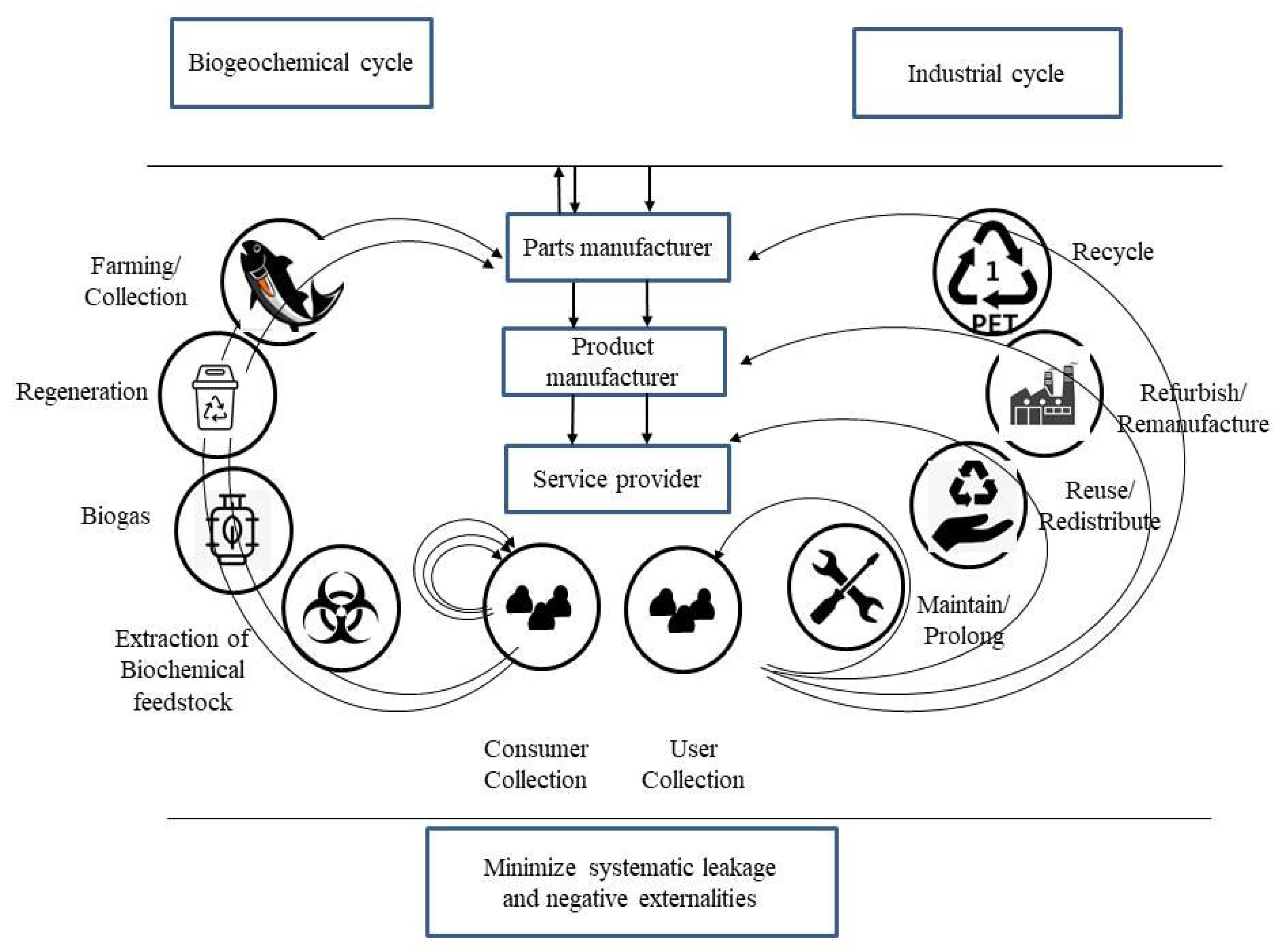
- Product design therefore determines the circularity potential of a product and includes the longevity, reparability, recyclability, proportion of recycled and renewable material in the product, and its suitability for refurbishment or remanufacture;
- In most finished products, the ratio of ETO components is a critical element to increase manufacturer’s profit, .
- Setup cost ();
- Holding cost ();
- Rework costs ();
- Production costs ();
- Case 1: (With I4.0 technology)
- Case 2: (Without I4.0 technology)
- (a)
- If , then the solution which minimizes not only exists but also is unique, and .
- (b)
- If , then optimal value of is . The production system should not be opened.
| Algorithm 1: Optimal solution of inventory problem. |
| 1: STEP 1: Start with and ;
2: STEP 2: Put into Equation (15) to obtain the corresponding value of and then from Equation (16) to calculate 3: STEP 3: If , put into Equation (16) to obtain the corresponding value of , i.e., otherwise, let ; 4: STEP 4: If the difference between and is sufficiently small, set . Otherwise, set , where is any small positive number, and set ; then, go back to STEP 2; 5: STEP 5: Substitute and into Equation (10) to calculate the value of . The objective is to determine the optimal the number of shipments, lot size per shipment and capital expenditure that minimizes the joint total expected cost per unit time of the integrated supply chain. |
4. Application Example
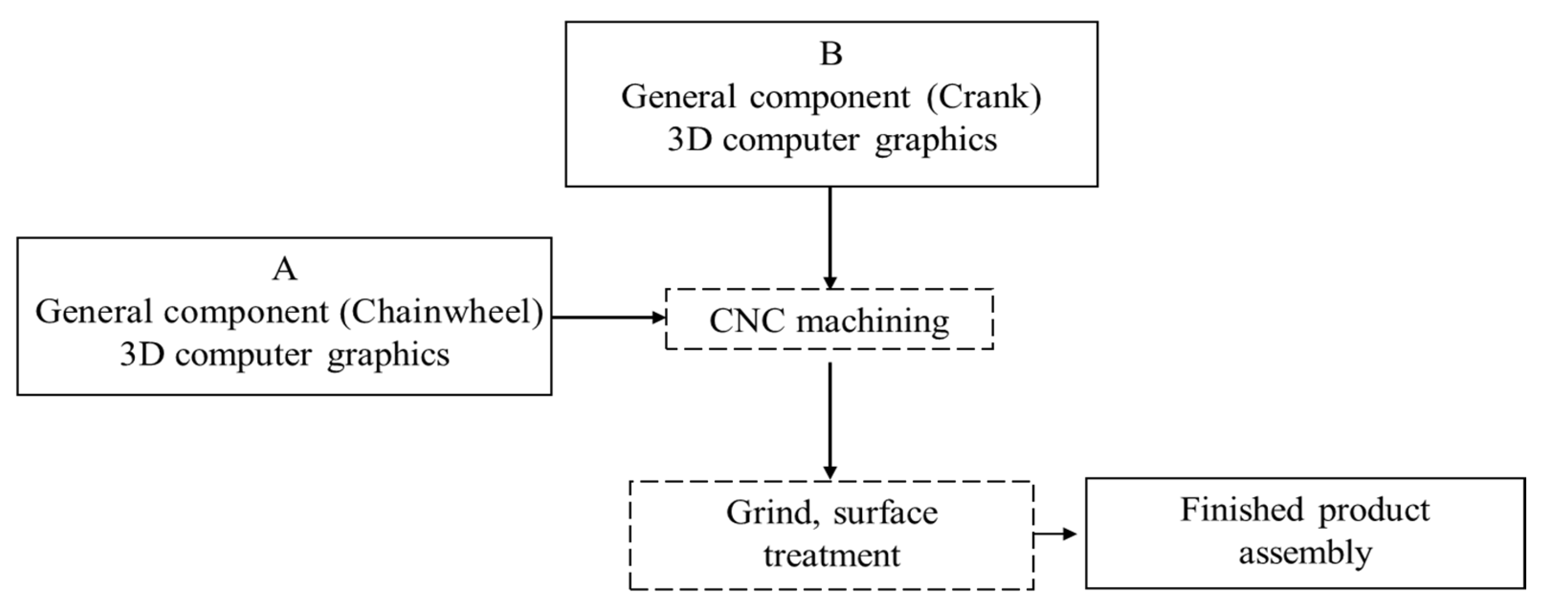
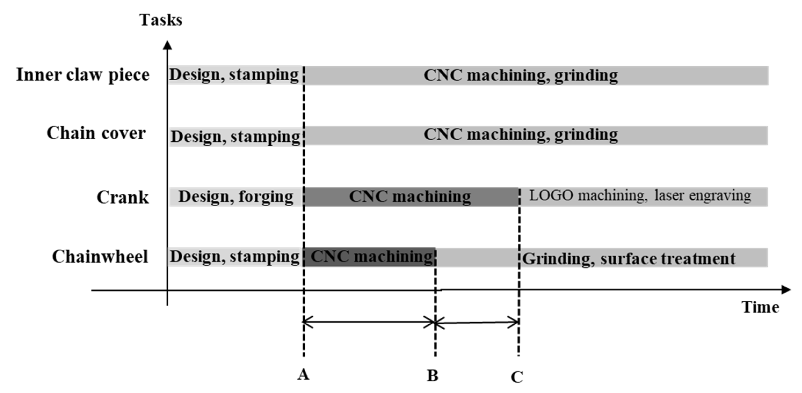
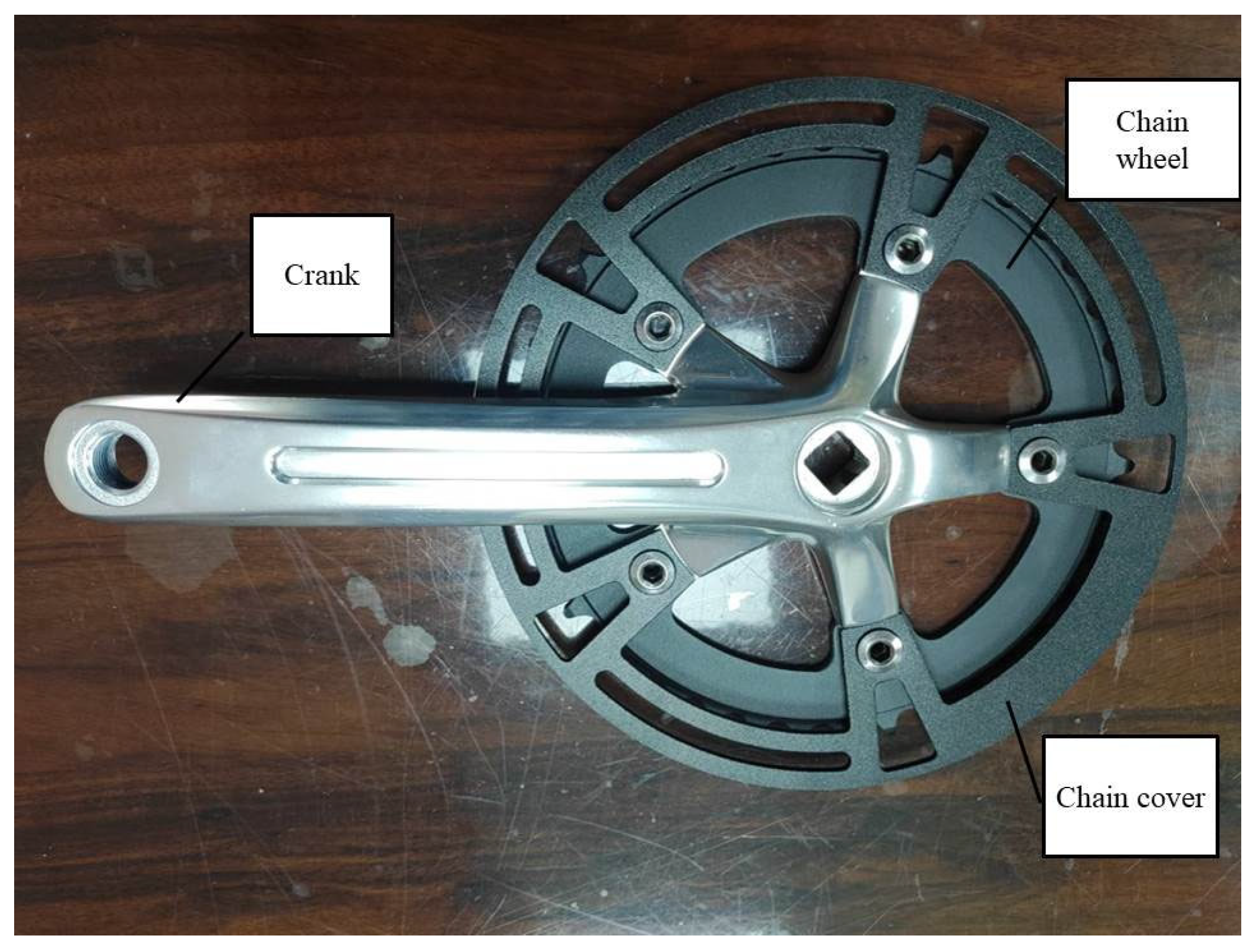
4.1. CE in the Context of a Bike Company
4.2. Numerical Example
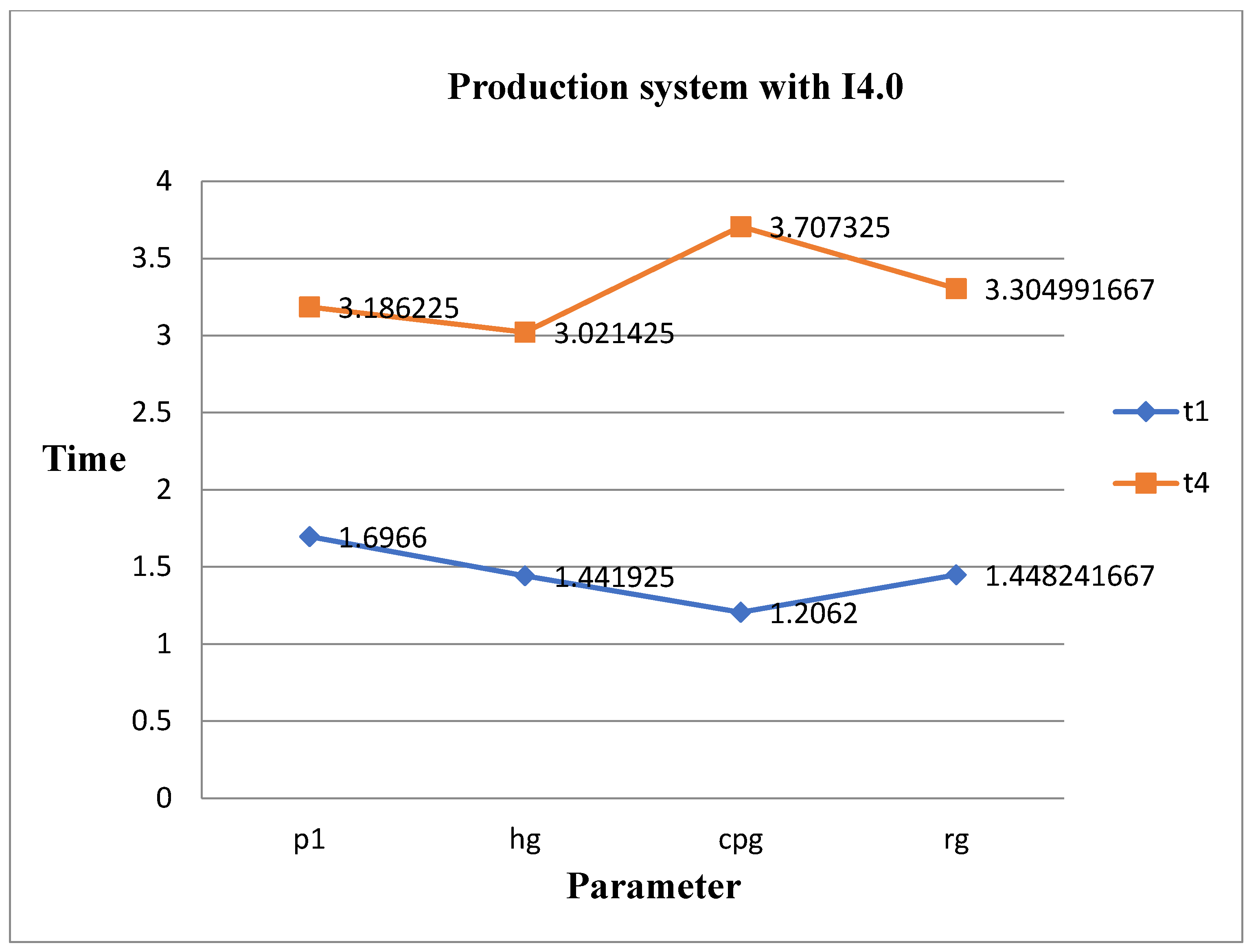
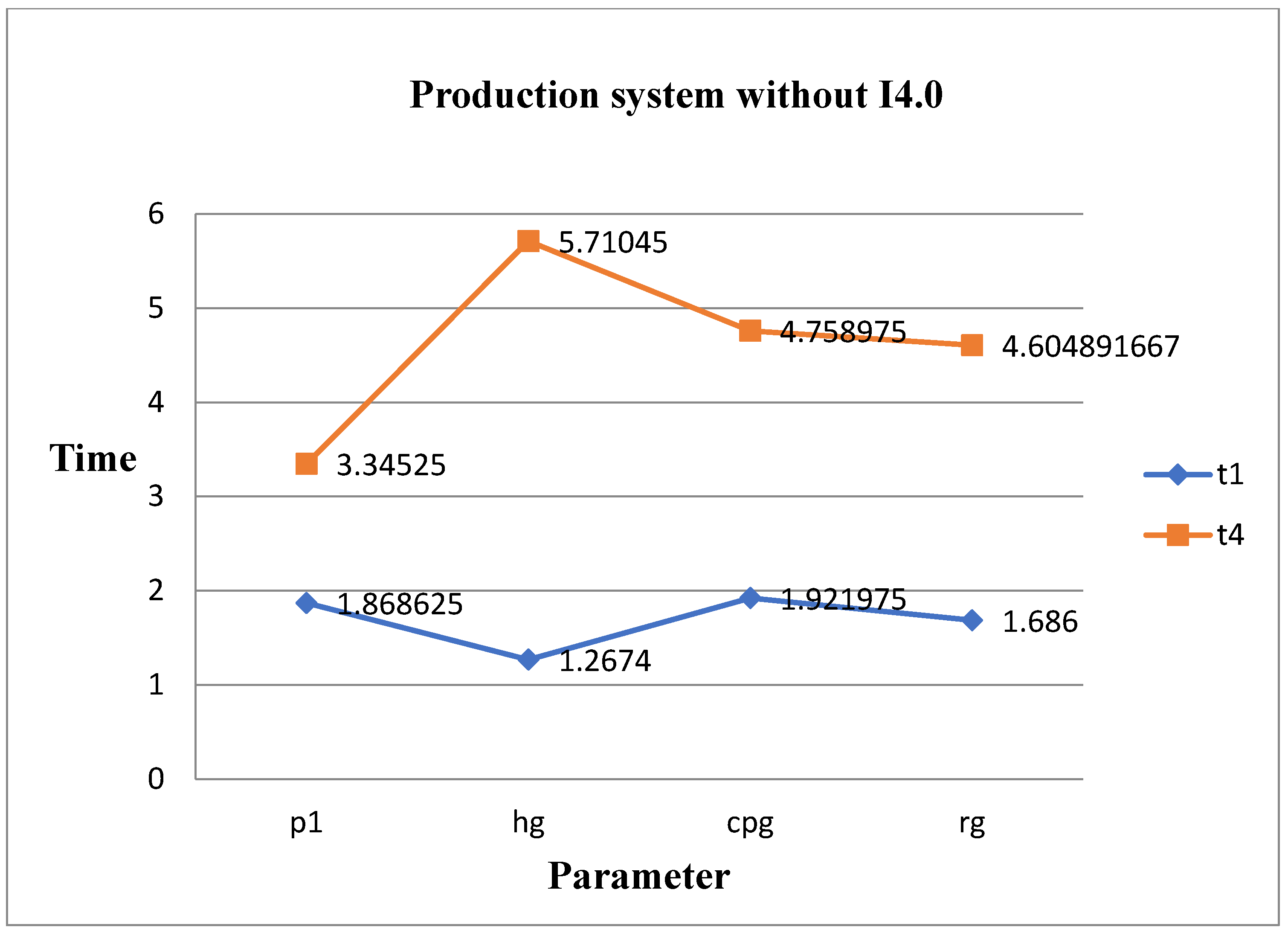
4.3. Sensitivity Analysis
5. Conclusions
Author Contributions
Funding
Institutional Review Board Statement
Informed Consent Statement
Data Availability Statement
Acknowledgments
Conflicts of Interest
Appendix A

| production rate for general component. | |
| demand rate per unit time. | |
| buyer’s ordering cost per order. | |
| design cost for general component per unit time. | |
| design cost for ETO component per unit time. | |
| purchase cost for finished product per unit time. | |
| purchase cost for general component per unit time. | |
| purchase cost for ETO component per unit time. | |
| defective rate for finished product. | |
| defective rate for ETO component. | |
| defective rate for general component. | |
| design fee (installment/payment). | |
| finished product with a ratio of ETO-based components. | |
| percentage for designing ETO-based components. | |
| holding cost for finished products per unit time. | |
| holding cost for general component per unit time. | |
| holding cost for ETO component per unit time. | |
| rework cost for finished products per unit time. | |
| rework cost for general component per unit time. | |
| rework cost for ETO component per unit time. | |
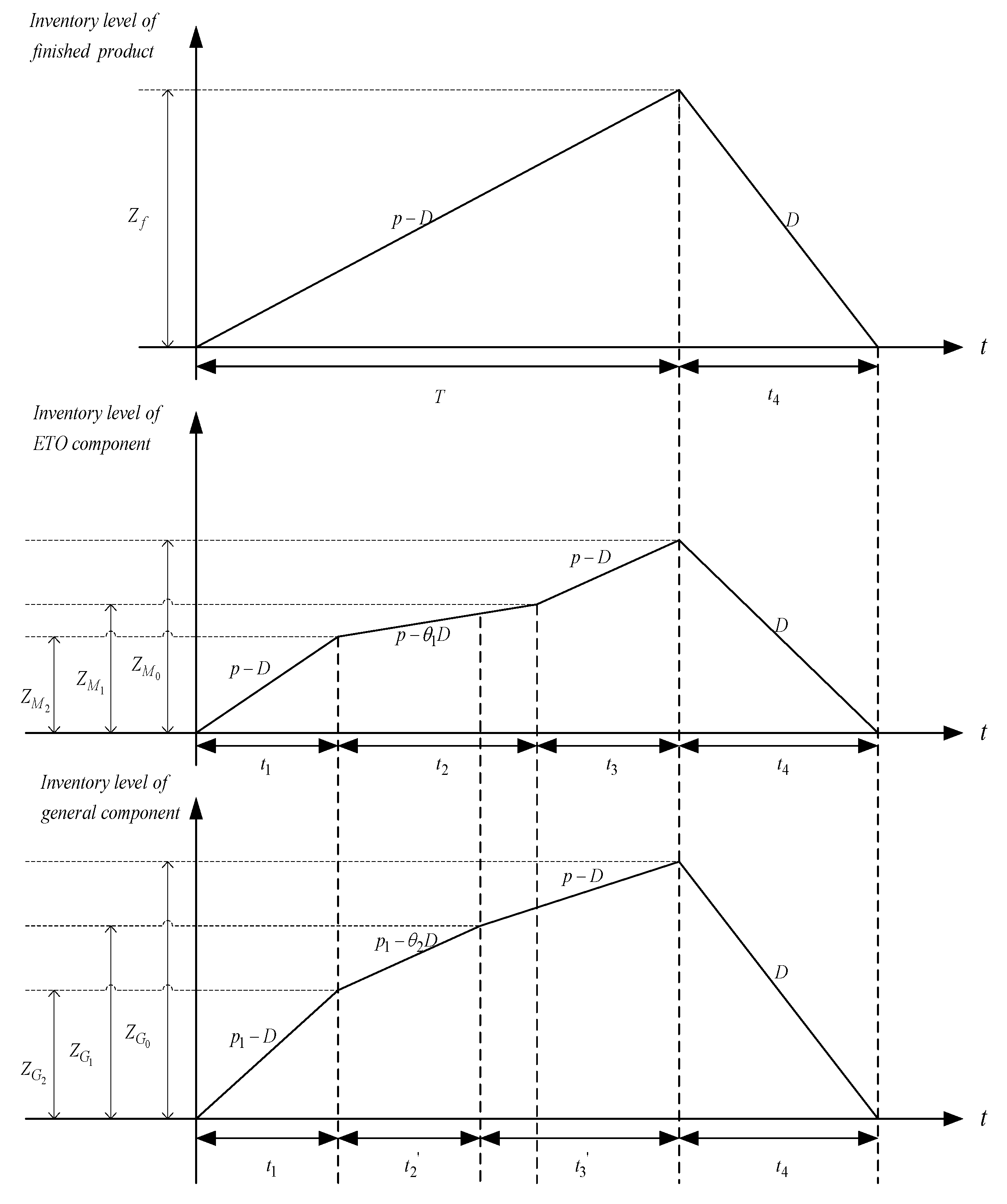
| maximum inventory level of finished products. | |
| maximum inventory level of ETO component can be assembled. | |
| maximum inventory level of general component can be CNC machined. | |
| maximum inventory level of general component can be stamped. | |
| time period prior to begin to CNC machining for ETO components in stage 2. | |
| time period prior to begin to surface finishing for ETO components in stage 2. |
| production rate of ETO components in stage 1. | |
| design time of general components in stage 1. | |
| time period of advertising and sales promotions in stage 2 (the maturity stage). |
Appendix B
- (a)
- From, Equation (16), there exists a unique solution if . Furthermore, we derive the following differential equations and the determinant of the Hessian matrix, det (H) at the stationary point in order to examine the second-order sufficient conditions (SOSC) for a minimum value. Taking the second partial derivatives of with respect to and , respectively, yields.andTherefore, we can determine the nature of stationary point by considering value of Hessian matrix and whether Hessian is negative definite.
- (b)
- From Equation (11), for , we obtain that . This implies that a large value of causes a higher value of . Hence, the minimum value of occurs at the point . It seems reasonable to conclude that the production system will not be opened. This completes the proof. □
References
- Gillan, S.L.; Koch, A.; Starks, L.T. Firms and social responsibility: A review of ESG and CSR research in corporate finance. J. Corp. Financ. 2021, 66, 101889. [Google Scholar] [CrossRef]
- Taft, E.W. The most economical production lot. Iron Age 1918, 101, 1410–1412. [Google Scholar]
- Harris, F.W. How many parts to make at once. Oper. Res. 1990, 38, 947–950. [Google Scholar] [CrossRef]
- Taleizadeh, A.A.; Soleymanfar, V.R.; Govindan, K. Sustainable economic production quantity models for inventory systems with shortage. J. Clean Prod. 2018, 174, 1011–1020. [Google Scholar] [CrossRef]
- Karim, R.; Nakade, K. A literature review on the sustainable EPQ model, focusing on carbon emissions and product recycling. Logistics 2022, 6, 55. [Google Scholar] [CrossRef]
- Arslan, M.C.; Turkay, M. EOQ revisited with sustainability considerations. Found. Comput. Decis. Sci. 2013, 38, 223–249. [Google Scholar] [CrossRef]
- Ganesan, S.; Uthayakumar, R. Optimisation of a sustainable fuzzy EPQ inventory model using sextic equation. Eur. J. Ind. Eng. 2022, 16, 442–478. [Google Scholar] [CrossRef]
- Jiaqi, Z.; Meizhang, H. Product sustainable design information model for remanufacturing. Int. J. Adv. Manuf. Technol. 2022; forthcoming. [Google Scholar] [CrossRef]
- Digiesi, S.; Mossa, G.; Rubino, S. A sustainable EOQ model for repairable spare parts under uncertain demand. IMA J. Manag. Math. 2015, 26, 185–203. [Google Scholar] [CrossRef]
- Ouyang, L.Y.; Yang, C.T.; Kao, A.; Huang, J.Z. Applying game theory to competitive production-inventory models with vendor’s imperfect production processes and the condition of buyer’s exemption from inspection. Adv. Mat. Res. 2015, 1125, 601–607. [Google Scholar] [CrossRef]
- Ouyang, L.Y.; Su, C.H.; Ho, C.H.; Yang, C.T. Optimal ordering policy for an economic order quantity model with inspection errors and inspection improvement investment. Int. J. Inf. Manag. Sci. 2014, 25, 317–330. [Google Scholar]
- Chang, C.T.; Ouyang, L.Y.; Teng, J.T.; Lai, K.K.; Cárdenas-Barrón, L.E. Manufacturer’s pricing and lot-sizing decisions for perishable goods under various payment terms by a discounted cash flow analysis. Int. J. Prod. Econ. 2019, 218, 83–95. [Google Scholar] [CrossRef]
- Su, R.H.; Weng, M.W.; Yang, C.T. Effects of corporate social responsibility activities in a two-stage assembly production system with multiple components and imperfect processes. Eur. J. Oper. Res. 2020, 293, 469–480. [Google Scholar] [CrossRef]
- Chang, H.J.; Su, R.H.; Weng, M.W.; Yang, C.T. An economic manufacturing quantity model for a two-stage assembly system with imperfect processes and variable production rate. Comput. Ind. Eng. 2012, 63, 285–293. [Google Scholar] [CrossRef]
- Lin, H.J. Investing in transportation emission cost reduction on environmentally sustainable EOQ models with partial backordering. J. Appl. Sci. Eng. 2018, 21, 291–303. [Google Scholar]
- Arora, R.; Singh, A.P.; Sharma, R.; Chauhan, A. A remanufacturing inventory model to control the carbon emission using cap-and-trade regulation with the hexagonal fuzzy number. Benchmarking 2022, 29, 2202–2230. [Google Scholar] [CrossRef]
- Khan, M.A.A.; Cárdenas-Barrón, L.E.; Treviño-Garza, G.; Céspedes-Mota, A. Optimal circular economy index policy in a production system with carbon emissions. Expert. Syst. Appl. 2023, 212, 118684. [Google Scholar] [CrossRef]
- Priyan, S.; Mala, P.; Palanivel, M. A cleaner EPQ inventory model involving synchronous and asynchronous rework process with green technology investment. Clean. Logist. Supply Chain 2022, 4, 100056. [Google Scholar] [CrossRef]
- Stindt, D. A generic planning approach for sustainable supply chain management-How to integrate concepts and methods to address the issues of sustainability? J. Clean. Prod. 2017, 153, 146–163. [Google Scholar] [CrossRef]
- Liao, H.; Deng, Q. EES-EOQ model with uncertain acquisition quantity and market demand in dedicated or combined remanufacturing systems. Appl. Math. Model. 2018, 64, 135–167. [Google Scholar] [CrossRef]
- Condeixa, L.D.; Silva, P.; Moah, D.; Farias, B.; Leiras, A. Evaluation cost impacts on reverse logistics using an economic order quantity (EOQ) model with environmental and social considerations. Cent. Eur. J. Oper. Res. 2022, 30, 921–940. [Google Scholar] [CrossRef]
- Su, R.H.; Weng, M.W.; Yang, C.T.; Li, H.T. An imperfect production–inventory model with mixed materials containing scrap returns based on a circular economy. Processes 2021, 9, 1275. [Google Scholar] [CrossRef]
- Suzanne, E.; Absi, N.; Borodin, V. Towards circular economy in production planning: Challenges and opportunities. Eur. J. Oper. Res. 2020, 287, 168–190. [Google Scholar] [CrossRef]
- Ginga, C.P.; Ongpeng, J.M.C.; Daly, M.K.M. Circular economy on construction and demolition waste: A literature review on material recovery and production. Materials 2020, 13, 2970. [Google Scholar] [CrossRef]
- Patil, R.A.; Ghisellini, P.; Ramakrishna, S. Towards Sustainable Business Strategies for a Circular Economy: Environmental, Social and Governance (ESG) Performance and Evaluation. An Introduction to Circular Economy; Springer: Berlin/Heidelberg, Germany, 2021; pp. 527–554. [Google Scholar]
- Theeraworawit, M.; Suriyankietkaew, S.; Hallinger, P. Sustainable supply chain management in a circular economy: A bibliometric review. Sustainability 2022, 14, 9304. [Google Scholar] [CrossRef]
- Rabta, B. An economic order quantity inventory model for a product with a circular economy indicator. Comput. Ind. Eng. 2020, 140, 106215. [Google Scholar] [CrossRef]
- Hegedűs, D.; Longauer, D. Implementation of a circular supply chain model using reusable components in multiple product generations. Heliyon 2023, 9, e15594. [Google Scholar] [CrossRef]
- Doltsinis, S.; Ferreira, P.; Mabkhot, M.M.; Lohse, N. A decision support system for rapid ramp-up of industry 4.0 enabled production systems. Comput. Ind. 2020, 116, 103190. [Google Scholar] [CrossRef]
- Tsao, Y.C.; Lee, P.L.; Liao, L.W.; Zhang, Q.; Vu, T.L.; Tsai, J. Imperfect economic production quantity models under predictive maintenance and reworking. Int. J. Syst. Sci. Oper. Logist. 2020, 7, 347–360. [Google Scholar] [CrossRef]
- Fatimah, Y.; Govindan, A.K.; Murniningsih, R.; Setiawan, A. Industry 4.0 based sustainable circular economy approach for smart waste management system to achieve sustainable development goals: A case study of Indonesia. J. Clean. Prod. 2020, 269, 122–169. [Google Scholar] [CrossRef]
- Fernandes, J.A.L.; Sousa-Filho, J.M.; Viana, F.L.E. Sustainable business models in a challenging context: The amana katu case. Rev. Adm. Contemp. 2021, 25, 1–17. [Google Scholar] [CrossRef]
- Jabbour, C.J.C.; Fiorini, P.D.C.; Ndubisi, N.O.; Queiroz, M.M.; Piato, É.L. Digitally-enabled sustainable supply chains in the 21st century: A review and a research agenda. Sci. Total. Environ. 2020, 725, 138177. [Google Scholar] [CrossRef]
- Julianelli, V.; Caiado, R.G.G.; Scavarda, L.F.; de Cruz, S.P.M.F. Interplay between reverse logistics and circular economy: Critical success factors-based taxonomy and framework. Resour. Conserv. Recycl. 2020, 158, 104–132. [Google Scholar] [CrossRef]
- Queiroz, M.M.; Fosso-Wamba, S.; Machado, M.C.; Telles, R. Smart production systems drivers for business process management improvement: An integrative framework. Bus. Process. Manag. J. 2020, 26, 1075–1092. [Google Scholar] [CrossRef]
- Scarpellini, S.; Valero-Gil, J.; Moneva, J.M.; Andreaus, M. Environmental management capabilities for a “circular eco-innovation”. Bus. Strategy. Environ. 2020, 3, 1850–1864. [Google Scholar] [CrossRef]
- Kristoffersen, E.; Mikalef, P.; Blomsma, F.; Li, J. The effects of business analytics capability on circular economy implementation, resource orchestration capability, and firm performance. Int. J. Prod. Econ. 2021, 239, 108205. [Google Scholar] [CrossRef]
- Sehnem, S.; de Queiroz, A.A.F.S.; Pereira, S.C.F.; dos Santos Correia, G.; Kuzma, E. Circular economy and innovation: A look from the perspective of organizational capabilities. Bus. Strategy Environ. 2021, 31, 236–250. [Google Scholar] [CrossRef]
- Cagno, E.; Neri, A.; Negri, M.; Bassani, C.A.; Lampertico, T. The role of digital technologies in operationalizing the circular economy transition: A systematic literature review. Appl. Sci. 2021, 11, 3328. [Google Scholar] [CrossRef]
- Macioszek, E.; Cieśla, M. External environmental analysis for sustainable bike-sharing system development. Energies 2022, 15, 791. [Google Scholar] [CrossRef]
- Macioszek, E.; Granà, A. The analysis of the factors influencing the severity of bicyclist injury in bicyclist-vehicle crashes. Sustainability 2022, 14, 215. [Google Scholar] [CrossRef]
- Huang, Y.F.; Weng, M.W.; Hoàng, T.T.; Lai, I.S. Circular economy policy of bike industry-exploring the optimal ETO component under imperfect production processes system. In Proceedings of the 2021 IEEE International Conference on Social Sciences and Intelligent Management (SSIM), Taichung, Taiwan, 29–31 August 2021. [Google Scholar] [CrossRef]
- Taiwan Excellence Award. Taiwan Bicycle Industry Growing at Fast Pace. 2022. Available online: https://www.businesswire.com/news/home/20220714005384/en/Taiwanese-Bicycle-Industry-Growing-at-Fast-Pace (accessed on 1 April 2023).
- Maleque, M.A.; Hossain, M.S.; Dyuti, S. Material properties and design aspects of folding bicycle frame. Adv. Mat. Res. 2011, 264, 777–782. [Google Scholar] [CrossRef]
- Gurjanov, A.V.; Zakoldaev, D.A.; Shukalov, A.V.; Zharinov, I.O. Principles of designing cyber-physical system of producing mechanical assembly components at Industry 4.0 enterprise. IOP Conf. Ser. Mater. Sci. Eng. 2018, 327, 022110. [Google Scholar] [CrossRef]
- Dutta, G.; Kumar, R.; Sindhwani, R. Digital transformation priorities of India’s discrete manufacturing SMEs-a conceptual study in perspective of Industry 4.0. Compet. Rev. Int. Bus. J. 2020, 30, 289–314. [Google Scholar] [CrossRef]
- Torn, I.A.R.; Vaneker, T.H.J. Mass personalization with industry 4.0 by SMEs: A concept for collaborative networks. Procedia Manuf. 2019, 28, 135–141. [Google Scholar] [CrossRef]


| References | Major Issues | Other Consideration(s) | ||||||
|---|---|---|---|---|---|---|---|---|
| EPQ/EOQ | Product | Demand | Supply Chain | En | E | S | ||
| Taleizadeh et al. [4] | EPQ | Single | Deterministic | Single | V | V | Single transportation mode, FIFO. | |
| Ouyang et al. [10] | EPQ | Single | Price-quality | Two-echelon | V | Game theory. | ||
| Ouyang et al. [11] | EOQ/EPQ | Single | Deterministic | Single | V | V | Inspection improvement investment. | |
| Chang et al. [14] | EPQ | Single | Deterministic | Single | V | V | V | Discounted cash flow. |
| Arora et al. [16] | EPQ | Single | Deterministic | Single | V | V | Cap-and-trade regulation. | |
| Khan et al. [17] | EPQ | Single | Cicular-index | Two-echelon | V | V | V | Carbon tax, circular economic index. |
| Stindt [19] | SSCM | Single | Deterministic | Two-echelon | V | V | Synthesize concepts and methods. | |
| Liao and Deng [20] | EOQ | Single | Uncertainty | Single | V | V | Carbon footprint. | |
| Condeixa et al. [21] | EOQ | Multiple | Deterministic | Single | V | V | V | Reverse logistics. |
| Su et al. [22] | EPQ | Multiple | Deterministic | Single | V | V | Green manufacturing (GM), scrap returns, CE. | |
| Rabta [27] | EOQ | Single | Linear form | Single | V | Circularity index. | ||
| Hegedűs and Longauer [28] | EOQ/EPQ | Single | Deterministic | Two-echelon | V | CE, sustainability. | ||
| Doltsinis et al. [29] | I4.0. | |||||||
| Tsao et al. [30] | EPQ | Multiple | Deterministic | I4.0, Corrective maintenance. | ||||
| This paper | EPQ | Single | Deterministic | Two-echelon | V | V | CE, I4.0. | |
| Example 1 (Case 1) | |||
| = 12,000 | = $0.5 | = $0.375 | = $0.4 |
| = $0.04 | = $0.03 | = $0.005 | = $10 |
| = $5 | = $7 | = 0.04 | = 0.03 |
| = 0.01 | = 0.2 | = 1 | |
| Example 2 (Case 2) | |||
| = 10,000 | = $0.5 | = $0.375 | = $0.4 |
| = $0.04 | = $0.03 | = $0.005 | = 0.3 |
| = 0.2 | = 0.1 | = 0.04 | = 0.03 |
| = 0.01 | = 0.2 | = 1 | |
| Parameter | Change (%) | Optimal Solutions | |||
|---|---|---|---|---|---|
| 50% | 436.98 | 1.0686 | 3.7668 | 4020.82 | |
| 25% | 419.47 | 1.1776 | 3.1692 | 3916.01 | |
| −25% | 362.76 | 1.8736 | 3.0194 | 2706.39 | |
| −50% | 278.78 | 2.6666 | 2.7895 | 2601.58 | |
| 50% | 337.439 | 1.9686 | 3.3733 | 3903.41 | |
| 25% | 344.952 | 1.8761 | 3.1449 | 3857.31 | |
| −25% | 446.238 | 0.8659 | 3.0315 | 2765.10 | |
| −50% | 451.165 | 0.8567 | 3.0256 | 2719.00 | |
| 50% | 394.441 | 1.1452 | 2.7618 | 3284.07 | |
| 25% | 394.957 | 1.1561 | 2.7758 | 3256.24 | |
| −25% | 399.771 | 1.6601 | 3.8019 | 2972.56 | |
| −50% | 399.592 | 1.6898 | 3.8199 | 2900.73 | |
| 50% | 383.598 | 1.1781 | 3.9862 | 2917.13 | |
| 25% | 386.711 | 1.1949 | 3.3030 | 2972.77 | |
| −25% | 425.238 | 1.6743 | 2.4454 | 3384.04 | |
| −50% | 430.651 | 1.7204 | 2.3511 | 3539.67 | |
| 50% | 402.703 | 1.1912 | 3.3701 | 3817.24 | |
| 25% | 399.703 | 1.2012 | 3.1701 | 3814.22 | |
| −25% | 391.703 | 1.2212 | 2.9701 | 3808.18 | |
| −50% | 382.703 | 1.2312 | 2.8701 | 3805.16 | |
| 50% | 502.322 | 1.2312 | 5.1512 | 2969.65 | |
| 25% | 457.434 | 1.2212 | 4.1232 | 2966.42 | |
| −25% | 348.447 | 1.1912 | 2.9871 | 2960.98 | |
| −50% | 300.512 | 1.1812 | 2.5678 | 2957.75 | |
| 50% | 406.568 | 2.1664 | 3.2438 | 3135.37 | |
| 25% | 401.717 | 1.3311 | 3.2384 | 2973.28 | |
| −25% | 379.631 | 0.9036 | 1.1935 | 2649.12 | |
| −50% | 344.729 | 0.6090 | 1.1775 | 2487.04 | |
| 50% | 401.325 | 1.2071 | 3.9700 | 2963.24 | |
| 25% | 399.172 | 1.2092 | 3.7712 | 2963.24 | |
| −25% | 396.091 | 1.2112 | 2.9189 | 2962.02 | |
| −50% | 392.858 | 1.2134 | 2.8650 | 2961.84 | |
| 50% | 398.501 | 1.2108 | 3.0691 | 2963.24 | |
| 25% | 398.603 | 1.2111 | 3.0698 | 2963.14 | |
| −25% | 398.901 | 1.2115 | 3.0710 | 2963.03 | |
| −50% | 398.921 | 1.2118 | 3.0720 | 2963.02 | |
| 50% | 398.751 | 1.2106 | 3.0722 | 2963.04 | |
| 25% | 398.721 | 1.2107 | 3.0712 | 2963.04 | |
| −25% | 398.681 | 1.2116 | 3.0691 | 2963.03 | |
| −50% | 398.661 | 1.2118 | 3.0682 | 2963.01 | |
| 50% | 399.891 | 1.2108 | 3.0901 | 2963.05 | |
| 25% | 399.822 | 1.2109 | 3.0802 | 2963.05 | |
| −25% | 397.401 | 1.2114 | 3.0603 | 2963.01 | |
| −50% | 396.301 | 1.2115 | 3.0401 | 2962.99 | |
| 50% | 398.901 | 1.2107 | 3.0712 | 2963.12 | |
| 25% | 398.821 | 1.2109 | 3.0708 | 2963.09 | |
| −25% | 398.711 | 1.2115 | 3.0698 | 2963.04 | |
| −50% | 398.612 | 2.2118 | 3.0691 | 2963.01 | |
| 50% | 398.691 | 1.2116 | 3.0691 | 2973.04 | |
| 25% | 398.692 | 1.2114 | 3.0697 | 2963.04 | |
| −25% | 398.705 | 1.2109 | 3.0705 | 2953.04 | |
| −50% | 398.708 | 1.2106 | 3.0709 | 2943.04 | |
| 50% | 402.145 | 1.1812 | 6.1934 | 3213.26 | |
| 25% | 401.178 | 1.1934 | 4.1980 | 3014.16 | |
| −25% | 396.013 | 1.2319 | 2.1982 | 2960.15 | |
| −50% | 392.124 | 1.2681 | 1.7841 | 2958.11 | |
| 50% | 412.013 | 1.2601 | 3.2146 | 5019.21 | |
| 25% | 401.456 | 1.2213 | 3.1561 | 4311.09 | |
| −25% | 381.781 | 1.1927 | 2.9811 | 1865.19 | |
| −50% | 361.890 | 1.1789 | 2.8157 | 1618.01 | |
| Parameter | Change (%) | Optimal Solutions | |||
|---|---|---|---|---|---|
| 50% | 125.399 | 3.0843 | 4.1282 | 6621.91 | |
| 25% | 393.338 | 2.9481 | 3.3552 | 6575.74 | |
| −25% | 516.398 | 0.7995 | 3.0995 | 6483.41 | |
| −50% | 553.813 | 0.6426 | 2.7981 | 6437.24 | |
| 50% | 199.344 | 0.9985 | 5.7014 | 6623.82 | |
| 25% | 298.280 | 1.0294 | 4.1272 | 6576.71 | |
| −25% | 530.233 | 1.1246 | 3.1402 | 6524.14 | |
| −50% | 539.372 | 1.9993 | 3.0511 | 6515.32 | |
| 50% | 157.571 | 1.0023 | 1.4074 | 6786.60 | |
| 25% | 160.434 | 1.0748 | 3.3701 | 6657.23 | |
| −25% | 526.985 | 1.0975 | 4.3503 | 6400.21 | |
| −50% | 541.887 | 1.1898 | 6.1973 | 6398.50 | |
| 50% | 71.7052 | 0.9946 | 1.9803 | 6476.52 | |
| 25% | 191.372 | 1.0172 | 2.3185 | 6503.91 | |
| −25% | 446.400 | 1.0929 | 8.9382 | 6553.54 | |
| −50% | 612.191 | 1.9649 | 9.6048 | 6579.21 | |
| 50% | 119.715 | 1.0010 | 3.1432 | 6532.77 | |
| 25% | 166.646 | 1.0272 | 3.6996 | 6529.47 | |
| −25% | 519.728 | 2.9220 | 4.1268 | 6526.28 | |
| −50% | 529.365 | 3.0534 | 5.0842 | 6524.67 | |
| 50% | 119.714 | 2.9419 | 1.1438 | 6532.98 | |
| 25% | 119.718 | 2.9368 | 1.1395 | 6531.28 | |
| −25% | 585.505 | 0.9148 | 0.3861 | 6527.87 | |
| −50% | 591.946 | 0.8944 | 0.3665 | 6526.16 | |
| 50% | 411.648 | 1.0000 | 8.8623 | 6672.35 | |
| 25% | 507.545 | 1.0269 | 4.4774 | 6600.96 | |
| −25% | 619.926 | 2.2554 | 2.4523 | 6458.18 | |
| −50% | 620.329 | 2.5789 | 1.7692 | 6386.79 | |
| 50% | 119.721 | 2.9318 | 3.1282 | 6529.61 | |
| 25% | 279.927 | 2.0342 | 3.4481 | 6529.59 | |
| −25% | 523.091 | 1.0318 | 4.1386 | 6529.55 | |
| −50% | 591.721 | 0.9317 | 4.3503 | 6529.53 | |
| 50% | 959.383 | 0.9613 | 4.8483 | 6529.66 | |
| 25% | 617.581 | 1.0267 | 4.6210 | 6529.61 | |
| −25% | 217.586 | 1.0433 | 3.4905 | 6529.53 | |
| −50% | 225.004 | 1.0488 | 3.6877 | 6529.49 | |
| 50% | 268.496 | 1.0244 | 3.3183 | 6529.67 | |
| 25% | 351.181 | 1.0264 | 3.3222 | 6529.57 | |
| −25% | 905.177 | 1.0425 | 4.8095 | 6529.47 | |
| −50% | 952.832 | 1.0826 | 4.8479 | 6529.47 | |
| 50% | 419.583 | 1.3165 | 1.8924 | 6529.61 | |
| 25% | 495.711 | 1.2702 | 2.8304 | 6529.59 | |
| −25% | 529.404 | 0.8844 | 4.5494 | 6529.55 | |
| −50% | 628.991 | 0.8845 | 8.4646 | 6529.51 | |
| 50% | 398.901 | 1.2107 | 3.0712 | 2963.12 | |
| 25% | 398.821 | 1.2109 | 3.0708 | 2963.09 | |
| −25% | 398.711 | 1.2115 | 3.0698 | 2963.04 | |
| −50% | 398.612 | 2.2118 | 3.0691 | 2963.01 | |
| 50% | 210.182 | 1.0231 | 3.2298 | 6559.57 | |
| 25% | 363.959 | 1.0268 | 3.7892 | 6549.57 | |
| −25% | 519.721 | 2.9318 | 3.9761 | 6539.57 | |
| −50% | 569.489 | 3.0068 | 3.9911 | 6529.57 | |
| 50% | 436.780 | 1.1715 | 1.2687 | 6466.63 | |
| 25% | 502.420 | 1.0487 | 1.1120 | 6493.74 | |
| −25% | 573.259 | 0.9411 | 0.8959 | 6582.69 | |
| −50% | 646.242 | 0.7510 | 0.7197 | 6678.85 | |
| 50% | 363.959 | 1.0268 | 1.7892 | 6429.59 | |
| 25% | 500.011 | 1.0302 | 2.0055 | 6429.47 | |
| −25% | 530.111 | 1.9592 | 5.6479 | 6429.37 | |
| −50% | 619.721 | 2.9318 | 6.1352 | 6429.29 | |
| Parameter(s) | ||
|---|---|---|
| Customization-based interaction for ETO-based component can be complicated and small batch and multi-species order batch. | Enterprise offers flexibility in modeling ETO-based component, and build at a relatively fast pace, but must also be flexible and account for any design changes a customer may have. | |
| , , | Enterprise works with design for assembly (DFA) methods for different reasons. Some enterprises want to take cost out of their products, some want to make more products in their factories, and some want to simplify the product to increase quality and reliability. | Adding to this environment is the push for mass customization by consumers and purchasers of ETO products, requiring an already difficult process to move faster with a higher degree of customized design. |
| , , | When new activities occur (e.g., due to changes or defects), planned activities need to be replanned, including considering the consequences of such changes or delays for other activities from the customer’s specification. | A large number of defects usually occur in the initial stages of a project and early defect detection will lower the overall cost of the project. |
| , , | Defects, delays, disconnects (DDD) cause rework, repairs, returns (RRR) that consume valuable resources to contain problems, correct deviations, and restore customer relationships. | Liability for personal injuries caused by a product’s defective design can be imposed under several underlying legal theories, among them negligence, breach of warranty, and strict product liability. |
| , , | Products require limited custom design per customer order because they have standard designs that can be altered to fit the customer requirements. Products may even be manufactured using an MTO strategy. | The components also differ in degree of standardization, where some components are standardized and unaltered across many products and others may be changed and redesigned for each customer order. |
Disclaimer/Publisher’s Note: The statements, opinions and data contained in all publications are solely those of the individual author(s) and contributor(s) and not of MDPI and/or the editor(s). MDPI and/or the editor(s) disclaim responsibility for any injury to people or property resulting from any ideas, methods, instructions or products referred to in the content. |
© 2023 by the authors. Licensee MDPI, Basel, Switzerland. This article is an open access article distributed under the terms and conditions of the Creative Commons Attribution (CC BY) license (https://creativecommons.org/licenses/by/4.0/).
Share and Cite
Shen, C.-Y.; Huang, Y.-F.; Weng, M.-W.; Lai, I.-S.; Huang, H.-F. The Role of Industry 4.0 and Circular Economy for Sustainable Operations: The Case of Bike Industry. Appl. Sci. 2023, 13, 5986. https://doi.org/10.3390/app13105986
Shen C-Y, Huang Y-F, Weng M-W, Lai I-S, Huang H-F. The Role of Industry 4.0 and Circular Economy for Sustainable Operations: The Case of Bike Industry. Applied Sciences. 2023; 13(10):5986. https://doi.org/10.3390/app13105986
Chicago/Turabian StyleShen, Chiu-Yen, Yung-Fu Huang, Ming-Wei Weng, I-Sung Lai, and Hung-Fu Huang. 2023. "The Role of Industry 4.0 and Circular Economy for Sustainable Operations: The Case of Bike Industry" Applied Sciences 13, no. 10: 5986. https://doi.org/10.3390/app13105986