Dynamic Modeling and Analysis of a Driving Passenger Vehicle

Abstract

This study presents a dynamic model of a passenger vehicle and analyzes its dynamic characteristics and responses. A dynamic vehicle model with seven degrees of freedom was established to analyze the behavior of a driving vehicle. The vehicle model had three degrees of freedom for the sprung mass’s motion and four degrees for the unsprung masses. For this model, the equations of motion were derived using Lagrange’s equation. To verify the model, the suspension deformations computed using the model were compared with those measured through three actual vehicle driving tests: the slalom, double lane change, and step steer tests. Furthermore, we investigated the effects of suspension stiffness, suspension damping, and anti-roll bar torsional stiffness on the dynamic characteristics and responses of the vehicle model. This study presented a new full-car model that can analyze a turning vehicle’s behavior in response to changes in the steering angle input. The developed dynamic vehicle model may help vehicle designers predict the dynamic responses of a vehicle through simulation without performing a driving test.

1. Introduction

The ride comfort of vehicles has continuously improved in response to the diverse needs of consumers over the years. Previously, in degraded road environments, ride comfort was evaluated according to the behavior of a vehicle traveling on an uneven road surface. However, in recent years, when the road environment has improved, the behavior of the vehicle based on the steering wheel operation of the driver on a uniform road surface has also had a significant influence on the evaluation of riding comfort. To satisfy the riding comfort performance with the conditions mentioned above and consumers’ demand, automobile manufacturers have continuously conducted driving tests using numerous test vehicles from the past and have evaluated and improved ride comfort through the analysis of driving test results. However, the driving test process is time-consuming and expensive and involves the vehicle design stage, developing a prototype, and preparing and performing the test. In addition, variables such as external environmental factors during the driving test and the driver’s driving condition may adversely affect the reliability of the test. Therefore, to address the shortcomings and limitations of these driving tests, various studies are being conducted to establish a vehicle dynamics model and evaluate and improve riding comfort through simulations.

Vehicle dynamics have been studied by several researchers. Genta [1] presented the dynamic modeling of a vehicle and the dynamic behavior of the vehicle in some driving conditions, while Gillespie [2] presented the vehicle dynamics and balanced engineering with practical explanations of the performance of an automotive vehicle. Gillespie and Karamihas [3] examined the factors that must be considered in developing a simplified dynamic model for truck response to road roughness inputs. Meanwhile, the dynamics of tires and suspensions, which are vehicle parts, were also studied. Pacejka and Bakker [4] provided a set of mathematical formulae that accurately describe measured tire behavior and contain physically based formulations to calculate the forces and moments acting from road to tire during longitudinal, lateral, and camber slips. Dixon [5] provided comprehensive coverage of the design, installation, and utilization of a vehicle’s shock absorbers.

Based on the procedures of various driving tests, studies have been conducted to analyze ride comfort through the simulation of vehicle models. Accordingly, some notable studies related to driving tests are summarized. Choi et al. [6] experimentally measured and evaluated the vertical direction (bounce) and front-rear tilting (pitch) behavior of a vehicle body, which occurs predominantly when the vehicle passes through an uneven road surface during the test. Jonsson and Johansson designed a suspension system that can control bounce and pitch behavior to improve riding comfort [7]. On the other hand, the left and right tilting (roll) behavior of the vehicle body while turning on a flat road surface is also very important, considering ride comfort and stability. In this regard, Uys et al. [8] experimentally evaluated the roll behavior caused by changing the steering wheel of a driving vehicle. Additionally, Darling and Hickson [9] developed an anti-roll suspension system that can improve riding comfort by controlling roll behavior. Further, Choi et al. [10] performed an experiment suggesting a method to control the damping characteristics of the suspension. This method takes into account the distinct body bounce, pitch, and roll behaviors, which were previously examined individually in separate studies.

Several studies have been published on the analysis of ride comfort, utilizing simulation techniques that simplify vehicle systems into basic dynamic models These studies predominantly focus on the quarter-car model, which solely considers the vertical behavior of the vehicle body. Sun et al. [11] established a two-degree-of-freedom vehicle model with vertical road surface excitation and derived the equation of motion using the Lagrange equation. Subsequently, the vertical vibration of the vehicle body according to the change in parameters such as mass, stiffness, and damping ratio in the model was analyzed through numerical analysis. Georgiou et al. [12] presented an optimization technique for deriving optimum values of damping and stiffness of suspension for improved ride comfort with vehicle models, including manual and semi-active suspension. Singh et al. [13,14] established a model by additionally considering a seat and a human body in a quarter-car model that depicts only existing vehicles. They proposed a methodology to improve ride comfort through vibration responses from seats or body parts according to vertical road excitation.

After that, the vehicle model was expanded from the existing quarter-car model to the half-car model to consider the tilting behavior of the car body. Some studies that analyzed ride comfort using this model are as follows: Sun et al. [15] derived the equations of motion for a vehicle model with four degrees of freedom that can consider the bounce and pitch of the vehicle body traveling on a rough road. They analyzed various responses in the time and frequency domains for the change in model parameters. Zhu et al. [16] obtained frequency response functions for random road excitation through a vehicle model considering the pneumatically interconnected suspension (PIS) system and compared and analyzed them with the vehicle model without the PIS system. On the other hand, Hudha et al. [17] were interested in the roll behavior of the vehicle body. They established a vehicle model with the effects of the anti-roll bar and the control arm and presented a suspension control system that can control the roll of the vehicle body caused by road excitation. Gosselin-Brisson et al. [18] proposed an active anti-roll bar system that can effectively control the roll motion of the vehicle body caused by lateral acceleration under vehicle turning conditions.

Recent studies analyzed the riding comfort of a full-size car model to better understand the behavior of the actual vehicle. Abu Bakar et al. [19] proposed a full car model with seven degrees of freedom that can analyze ride comfort. To verify the validity of the proposed model, the similarity between the simulation and experimental results was shown in the pitch mode test condition of the vehicle body that occurs when passing through a bump. Palli et al. [20] and Sentilkumar et al. [21] established a full vehicle model with seven degrees of freedom considering active suspension and found that active suspension improves riding comfort by preventing vehicle resonance that may occur due to road excitation. On the other hand, Ghike and Shim [22] proposed a full car model with 14 degrees of freedom that can analyze the rolling behavior of a turning vehicle according to steering conditions. He also showed the limitations of his model and demonstrated its excellence and validity.

On the other hand, vehicle dynamics can be analyzed by using commercial multi-body dynamics software packages such as ANSYS-Motion [23], RecurDyn [24], MSC/Adams [25], and Simpack [26]. These commercial packages provide the advantage of easily constructing detailed vehicle models. However, they require a lot of experience and skill in constructing the model, assigning boundary conditions/constraints, and often requiring long computation times. On the contrary, concentrated mass models are difficult to apply to complex systems. However, it is relatively easy to analyze the influence of various parameters of the model and requires shorter computation times.

With improvements in the road environment and recent developments in the vehicle industry, vehicle consumers are demanding improvements in ride comfort performance according to the driver’s steering conditions rather than solely focusing on ride comfort performance against irregular road surface disturbances. In this regard, various vehicle manufacturers have attempted to analyze and improve ride comfort through driving tests. However, a time-efficient and affordable method is needed for driving tests to quickly respond to consumer demands. Therefore, building a simple mathematical model of a vehicle that can analyze the riding comfort of a vehicle driven by steering input through simulation is desired.

However, most of the previous studies investigated by the authors tend to focus on vehicle models for analyzing ride comfort under disturbance conditions, such as uneven road surfaces or irregularities. In addition, several studies have been published to analyze the behavior of the vehicle body by establishing a vehicle model for turning conditions. However, they have used a method to obtain a response generated by inputting an arbitrary lateral acceleration into the vehicle body. Since lateral acceleration is a variable determined by the change in steering angle input by the driver, it is limited as an actual input condition for a turning vehicle. In summary, the limitation of vehicle models in the previous studies is that they cannot analyze the dynamic responses of a turning vehicle according to the vehicle speed and steering angle controlled by a driver. Therefore, this study introduces a full-car model that can analyze the dynamic behavior of a turning vehicle according to the change in steering angle, which is the driver’s input condition. The new 7-DOF full-car model proposed in this study is valuable in that the simulation and driving test results for various steering conditions have been comparatively verified. The main contribution of this study is to present a full car model encompassing an anti-roll bar that can analyze the dynamic behavior of the variation of the steering angle controlled by a driver.

The remainder of this paper is organized as follows: In Section 2, a dynamic vehicle model that can analyze the behavior of a driving passenger car is developed. A vehicle model with seven degrees of freedom was established, considering the centrifugal force acting on the vehicle during turning and the torsional stiffness of the anti-roll bar. Based on this model, the equations of motion are derived using Lagrange’s equation. In Section 3, the established vehicle model is verified by comparing the vertical suspension deformations computed with the vehicle model with the deformations measured through actual vehicle driving tests. For comparison, three driving tests were performed: the slalom, double lane change, and step steer tests. In Section 4, the natural frequencies and mode shapes of the dynamic vehicle model are computed and analyzed using the developed vehicle model. Furthermore, the effects of changes in the design parameters on the dynamic response of the vehicle model were investigated. The considered design parameters were suspension stiffness, suspension damping, and anti-roll bar torsional stiffness. Finally, conclusions and a summary of this study’s results are presented in Section 5.

2. Dynamic Vehicle Model

In this section, a dynamic model of a vehicle that can analyze the behavior of a driving passenger car is presented. This study assumes that the speed of the vehicle is kept constant, and the driving direction of the vehicle is changed by the steering wheel. Under these assumptions, the vehicle does not accelerate in the longitudinal direction (direction of travel), but only in the lateral direction perpendicular to the traveling direction. This lateral acceleration imparts a centripetal force to the vehicle and maintains it on a turning trajectory.

The centrifugal force acting on the vehicle during turning is given by the following equation:

$$F=m_t\frac{V^2}{R}$$

(1)

where $m_t$ is the total mass of the vehicle, $V$ is the speed of the vehicle, and $R$ is the turning radius. When the vehicle is traveling at a constant speed, as long as the mass $m_t$ and speed $V$ are constant, the centrifugal force $F$ is determined by the turning radius $R$.

The relationship between the turning radius of the vehicle and the steering angle of the steering wheel was analyzed. First, the relationship between the vehicle’s turning radius and the steering angles of the front wheels can be derived from the Ackermann steering geometry [27], as shown in Figure 1. In Figure 1, point $O$ is the instantaneous turning center, $G$ is the center of mass of the vehicle, and $l_1$ and $l_2$ are the distances from the center of mass to the front and rear wheels, respectively. $w$ is the distance between the centers of the left and right wheels, and $L$ is the distance from the front wheel to the rear wheel. As shown in this figure, the position of the turning center $O$ coincides with the intersection of the extension line of the rear axle and the vertical lines inside and outside the front wheels. Accordingly, the steering angle of the inner front wheel, ${\delta }_i$ is formed by the extension line of the rear axle and a line perpendicular to the inner front wheel. Additionally, the steering angle of the outer wheel, ${\delta }_o$ is formed by the extension line and a line perpendicular to the outer front wheel. The distance $R$ from the turning center $O$ to the vehicle center of mass $G$ is called the turning radius, and the distance from the turning center $O$ to the center of the rear axle is expressed as $R_r$.

Thus, if the instantaneous turning center is determined geometrically, the turning radius $R$ can be expressed as the inner and outer front wheel steering angles, ${\delta }_i$ and ${\delta }_o$. The relationship between the steering angles of the inner and outer front wheels, the distance from the turning center to the center of the rear wheel axle, and the distance between the left and right wheels can be expressed by the following equations:

$$\tan {\delta }_i=\frac{L}{R_r-w/2}$$

(2)

$$\tan {\delta }_o=\frac{L}{R_r+w/2}$$

(3)

In general, as the steering angle is not large when the vehicle is traveling, the steering angles ${\delta }_i$ and ${\delta }_o$ are assumed to be small, and the turning radius $R$ is very large compared to the distance w between the centers of the left and right wheels. Therefore, in Equations (2) and (3), $\tan {\delta }_i$ and $\tan {\delta }_o$ can be approximated by ${\delta }_i$ and ${\delta }_o$, the distance from the turning center to the center of the rear wheel axle, $R_r$ can be replaced by the turning radius $R$, and the distance between the left and right wheels $w$ can be neglected. Denoting the average steering angles of the inner and outer front wheels by $\delta$, that is, $\delta =\left({\delta }_i+{\delta }_o\right)/2$, the turning radius of the vehicle is given by:

$$R=\frac{L}{\delta }$$

(4)

This equation implies that the turning radius $R$ is determined by the average steering angle of the front wheels $\delta$ and wheelbase distance $L$.

The centrifugal force applied to a turning vehicle can be obtained by substituting Equation (4) with Equation (1).

$$F=\frac{m_t{V}^2\delta }{L}$$

(5)

The average steering angle of the front wheels is determined by the steering ratio and steering wheel angle, which can be expressed by the following equation [28]:

$${\delta }_s=i_s\delta$$

(6)

where ${\delta }_s$ is the angle of the steering wheel and $i_s$ is the steering ratio of the steering wheel angle to the steering angle of the front wheels. The steering angle ratio $i_s$ is determined by the gear ratio of the steering linkage connecting the steering wheel and the front wheel, which is 15 for the target vehicle of this study. Finally, the centrifugal force applied to a turning vehicle is expressed as follows: vehicle mass $m_t$, vehicle speed $V$, wheelbase distance $L$, steering wheel angle ${\delta }_s$, and steering ratio $i_s$.

$$F=\frac{m_t{V}^2{\delta }_s}{i_{s}L}$$

(7)

Next, a dynamic vehicle model with seven degrees of freedom was established to analyze the behavior of a driving vehicle. As shown in Figure 2, the vehicle was modeled with one sprung mass and four unsprung masses, for a total of five rigid bodies, and the suspension, anti-roll bar, and tires were modeled as springs and dampers. In Figure 2, the vehicle’s forward direction is the negative x-axis direction. In addition, the y- and z-axes are parallel to the left and right directions and the up and down directions of the vehicle, respectively. The sprung mass is the total mass of a vehicle supported by the suspension, which includes the body, frame, engine, transmission, and internal components. The unsprung mass includes wheel axles, wheel bearings, wheel hubs, tires, drive shafts, springs, shock absorbers, and suspension links. The motion of the sprung mass is described by the bounce displacement of the mass center $Z$, the pitch angle $\phi$, and the roll angle $\theta$, while the motions of the unsprung masses are described by the vertical displacements of $z_1$, $z_2$, $z_3$ and $z_4$. In this study, the x-direction motion of the sprung mass is defined as a constant vehicle speed $V$. Since the vibration and yaw motion in the x and y directions are ignored, the motion of the sprung mass is defined by the bounce displacement, pitch angle, and roll angle.

As shown in Figure 2, the sprung mass has a roll motion that rotates about a roll axis parallel to the x-axis at a distance $h=476$ mm vertically from the center of mass [29]. This considers the phenomenon that the lateral centrifugal force acting on the center of mass of the vehicle body located at a distance $h$ from the roll axis generates a roll moment for the vehicle body when the vehicle turns to the right. The position of the roll axis changes with a very complex mechanism depending on the kinematics of the suspension links. However, in this study, the relative position of the roll axis to the body is considered fixed to establish a simple and efficient model. Therefore, the roll moment $M_r$ shown in Figure 2 is expressed as the product of the centrifugal force $F$ applied to the vehicle and the distance $h$ from the roll axis to the mass center, that is, $M_r=Fh$.

The sprung mass has mass $m_s$, mass moment of inertia about the center of mass $I_x$, and mass moment of inertia about the y-axis $I_y$. The mass center of the sprung mass $G$ is located at a distance $l_1=1.07 \mathrm{m}$ from the front of the vehicle, $l_2=1.579 \mathrm{m}$ from the rear, $w_1=0.734 \mathrm{m}$ from the left end of the vehicle, and $w_2=0.824 \mathrm{m}$ from the right end of the vehicle. The front unsprung masses with mass $m_f$ have vertical displacements $z_1$ and $z_2$, while the rear unsprung masses with mass $m_r$ have displacements $z_3$ and $z_4$. However, experimentally obtaining the mass and mass moment of inertia values of various parts to calculate the inertia parameters of the model shown in Figure 2 is a time-consuming and complicated procedure. Therefore, in this study, the inertial values of the sprung and unsprung masses for the dynamic vehicle model were extracted from the 3-D solid model of the vehicle using commercial CAD software. These are the values: $m_s=1568$ kg, $m_f=47$ kg, $m_r=31$ kg, $I_x=719$ kg·m², and $I_y=2495$ kg·m². The products of inertia were neglected in this study because they were relatively small.

The suspension, tire, and anti-roll bar that connect the rigid body and ground defined above were modeled with linear equivalent springs and dampers. The front suspensions vertically connected between the sprung mass and front unsprung masses were modeled with an equivalent stiffness $k_f$ and an equivalent damping coefficient $c_f$. Additionally, the rear suspension vertically connected between the sprung mass and rear unsprung masses was modeled with an equivalent stiffness $k_r$ and equivalent damping coefficient $c_r$. As the tires between the ground and the unsprung masses have very high stiffness, they are modeled with an equivalent stiffness $k_t$ without damping.

On the other hand, anti-roll bars, which help reduce vehicle body roll in fast cornering or on irregular roads, are modeled as torsion springs. The bars are long U-shaped metals with hollow cross sections that join the suspensions on the right and left sides of an axle. They are usually attached to the chassis at two points using rubber bushings. 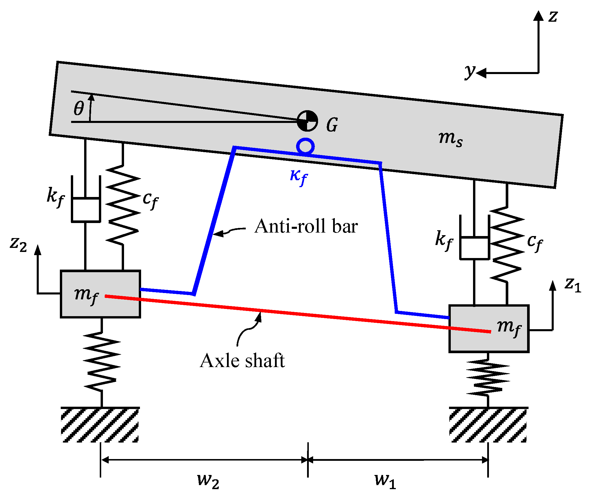The torsional stiffnesses of the front and rear anti-roll bars were assumed to be ${\kappa }_f$ and ${\kappa }_r$, respectively [30]. The twist angles of the anti-roll bars were determined by the angular displacements of the axel shafts relative to the sprung mass. The axle shaft has an angular displacement owing to the difference between the right and left wheels. To help understand this, a dynamic vehicle model viewed from the front is shown in Figure 3 as an example.

As the front left and right unsprung masses have vertical displacements $z_1$ and $z_2$, respectively, the angular displacement of the front axle shaft is computed as ${\tan }^{-1}\left[\left(z_2-z_1\right)/\left(w_1+w_2\right)\right]$. Therefore, the twist angle of the front anti-roll bar ${\varphi }_f$, is given by

$${\varphi }_f={\tan }^{-1}\left(\frac{z_2-z_1}{w_1+w_2}\right)-\theta$$

(8)

Similarly, the twist angle of the rear anti-roll bar can be expressed as

$${\varphi }_r={\tan }^{-1}\left(\frac{z_4-z_3}{w_1+w_2}\right)-\theta$$

(9)

The equivalent stiffness and damping coefficients presented above were calculated using an experimental method. The equivalent stiffness values of the suspensions and tires were obtained through static vertical load-deflection tests [31,32]. Similarly, the equivalent torsional stiffness values of the anti-roll bars were obtained through torsional load-torsion angular deformation tests. The values for the various equivalent stiffness, equivalent torsional stiffness, and damping coefficients obtained by the tests were as follows: $k_f=44,400$ N/m, $k_r=36,000$ N/m, $k_t=255,487$ N/m, ${\kappa }_f=62,085$ N·m/rad, ${\kappa }_r=58,098$ N·m/rad, and $c_f=c_r=5000$ N·s/m.

The equations of motion for the driving vehicle were derived using the following Lagrange equation:

$$\begin{gathered} \frac{\mathrm{d}}{\mathrm{dt}}\left(\frac{\partial T}{\partial {\dot{q}}_k}\right)+\frac{\partial F_d}{\partial {\dot{q}}_k}-\frac{\partial T}{\partial q_k}+\frac{\partial V}{\partial q_k}=Q_k \\ \mathrm{for} k=Z, \theta , \phi , z_1, z_2, z_3, z_4 \end{gathered}$$

(10)

where the superposed dot represents differentiation with respect to time; $q_k$ stands for the seven generalized coordinates; $T$, $V$, $F_d$ and $Q_k$ are the kinetic energy, potential energy, Rayleigh’s dissipation function, and generalized force, respectively. Among the generalized coordinates, the three coordinates ($Z$, $\theta$, and $\phi$) are for the motion of the sprung mass, whereas the four coordinates ($z_1$, $z_2$, $z_3$, $z_4$) are for the motions of the unsprung masses.

First, the kinetic energy of the dynamic vehicle model can be expressed as the following equation:

$$T=\frac{1}{2}{m}_s{\dot{Z}}^2+\frac{1}{2}{I}_x{\dot{\theta }}^2+\frac{1}{2}{I}_y{\dot{\phi }}^2+\frac{1}{2}{m}_f\left({\dot{z}}_1^2+{\dot{z}}_2^2\right)+\frac{1}{2}{m}_r\left({\dot{z}}_3^2+{\dot{z}}_4^2\right)$$

(11)

where the first term is for the translational motion of the sprung mass, the second and third terms are for the rotational motion of the sprung mass, and the fourth and fifth terms are for the translational motions of the unsprung masses.

Next, the potential energy owing to the deformations of the springs and torsional springs in the dynamic vehicle model may be given by

$$V=\frac{1}{2}{k}_t{\displaystyle \sum }_{i=1}^4{z}_i^2+\frac{1}{2}{k}_f\left(d_1^2+d_2^2\right)+\frac{1}{2}{k}_r\left(d_3^2+d_4^2\right)+\frac{1}{2}{\kappa }_f{\varphi }_f^2+\frac{1}{2}{\kappa }_r{\varphi }_r^2$$

(12)

where the first term is the potential energy of the tire, the second and third terms are the potential energies of the suspensions, and the fourth and fifth terms are the potential energies of the anti-roll bars. In the second and third terms, $d_1$, $d_2$, $d_3$, and $d_4$ are the suspension deformations at the left front wheel, right front wheel, left rear wheel, and right rear wheel, respectively.

The suspension deformation at each wheel, $d_i$ for i = 1, 2, 3, 4, is determined by subtracting the displacement of the unsprung mass from the z-directional displacement of the sprung mass at the point corresponding to each suspension. The displacement of the sprung mass at the left–front suspension, ${\mathbf{x}}_1$, displacement at the right–front suspension, ${\mathbf{x}}_2$, displacement at the left–rear suspension, ${\mathbf{x}}_3$, and displacement at the right–rear suspension, ${\mathbf{x}}_4$, can be determined by

$$x_i=x_G+{\mathbf{T}}_{ \phi }{\mathbf{T}}_{ \theta }{\mathbf{P}}_{ i} \mathrm{for} i=1, 2, 3, 4$$

(13)

where $x_G$ is the displacement of the mass center of the sprung mass, $P_i$ is the position vector of the point on the spring mass corresponding to each suspension, and $T_{\theta }$ and $T_{\phi }$ are the rotation matrices about the $x$ and $y$ axes, respectively. The vectors and matrices in Equation (13) are given by

$$x_G=\left\{\begin{array}{c}0\\ 0\\ Z\end{array}\right\}, {\mathbf{P}}_{ 1}=\left\{\begin{array}{c}-l_1\\ -w_1\\ 0\end{array}\right\}, {\mathbf{P}}_{ 2}=\left\{\begin{array}{c}-l_1\\ w_2\\ 0\end{array}\right\}, {\mathbf{P}}_{ 3}=\left\{\begin{array}{c}{l}_2\\ -w_1\\ 0\end{array}\right\}, {\mathbf{P}}_{ 4}=\left\{\begin{array}{c}{l}_2\\ w_2\\ 0\end{array}\right\}$$

(14)

$${\mathbf{T}}_{ \theta }=\left[\begin{array}{ccc}1& 0& 0\\ 0& \cos \theta & \sin \theta \\ 0& -\sin \theta & \cos \theta \end{array}\right], {\mathbf{T}}_{ \phi }=\left[\begin{array}{ccc}\cos \phi & 0& -\sin \phi \\ 0& 1& 0\\ \sin \phi & 0& \cos \phi \end{array}\right]$$

(15)

In other words, the suspension deformations were obtained by subtracting the displacements of the corresponding unsprung mass $z_i$ from the z-directional components of $x_i$. Consequently, the suspension deformations can be expressed as

$$\begin{gathered} d_1=Z-z_1-w_1\sin \theta \cos \phi +l_1\sin \phi , d_2=Z-z_2+w_2\sin \theta \cos \phi +l_1\sin \phi , \\ {d}_3=Z-z_3-w_1\sin \theta \cos \phi -l_2\sin \phi , d_4=Z-z_4+w_2\sin \theta \cos \phi -l_2\sin \phi \end{gathered}$$

(16)

On the other hand, Rayleigh’s dissipation function for the vehicle model can be represented by

$$F_d=\frac{1}{2}{c}_f\left({\dot{d}}_1^2+{\dot{d}}_2^2\right)+\frac{1}{2}{c}_r\left({\dot{d}}_3^2+{\dot{d}}_4^2\right)$$

(17)

where ${\dot{d}}_i$ ($i=1$, $2$, $3$, $4$) are the time derivatives of the suspension deformations given by Equation (16). Finally, the non-conservative generalized forces of Equation (10) are given by

$$Q_{\theta }=M_r, Q_Z=Q_{\phi }=Q_{z_1}=Q_{z_2}=Q_{z_3}=Q_{z_4}=0$$

(18)

As shown in these equations, there are no generalized forces except for $Q_{\theta }$, and this generalized force $Q_{\theta }$ is the roll moment described above.

The equations of motion were obtained by substituting the kinetic energy (Equation (11)), potential energy (Equation (12)), Rayleigh’s dissipation function (Equation (17)), and generalized forces (Equation (18)) into the Lagrange equation (Equation (10)). The derived equations are nonlinear ordinary differential equations for generalized coordinates. Assuming that the roll and pitch angles are small, the nonlinear equation can be linearized. The linearized equations of motion can be written as a matrix–vector equation as follows:

$$\mathbf{M}\ddot{\mathbf{q}}+\mathbf{C}\dot{\mathbf{q}}+\mathbf{Kq}=\mathbf{f}$$

(19)

where the superposed dot represents differentiation with respect to time, $q$ is the displacement vector defined by $\mathrm{q}=\{\theta$, $\phi$, $Z$, $z_1$, $z_2$, $z_3$, ${\left.z_4\right\}}^{\mathrm{T}}$, $M$ is the mass matrix, $C$ is the damping matrix, $K$ is the stiffness matrix, and $f$ is the load vector defined by $\mathrm{f}=\{M_r{, 0, 0, 0, 0, 0, 0\}}^{\mathrm{T}}$.

3. Dynamics Model Verification

To verify the dynamic vehicle model proposed in this study, the vertical suspension deformations computed using the vehicle model were compared with the deformations measured through actual vehicle driving tests. The vehicle for the driving tests was a semi-midsize hatchback-type passenger car with the specifications mentioned above. This vehicle, with one driver on board, was driven at a constant speed of 100 km/h on an outdoor proving ground with a dry and flat road surface. Three types of driving tests were conducted according to ISO standards: the slalom test [33], the double lane change test [34], and the step steer test [35]. These tests are performed for three steering wheel angle variations, the details of which will be discussed later.

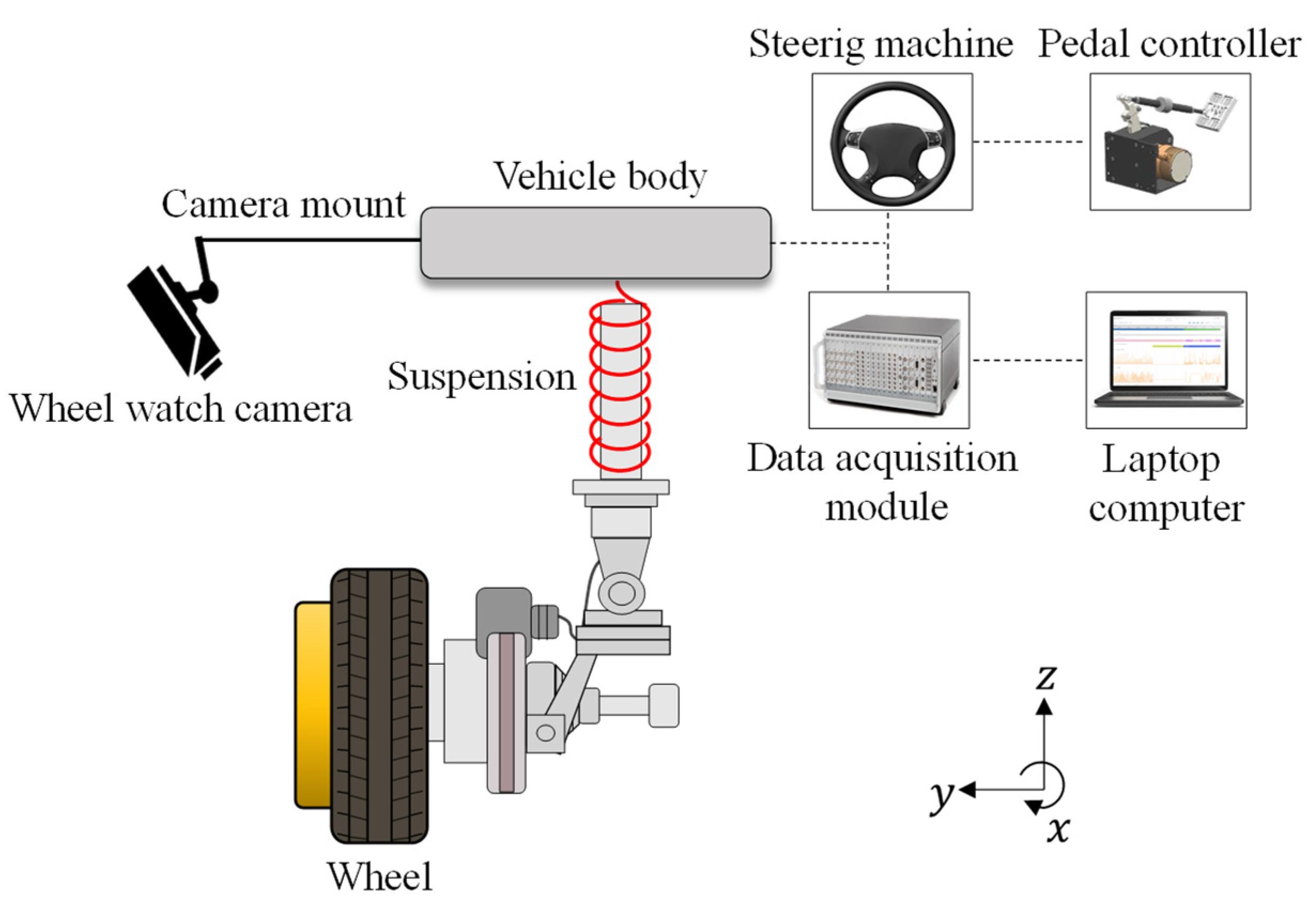
The experimental setup for measuring suspension deformations is shown in Figure 4. The pedal controller was used to maintain the vehicle’s speed at 100 km/h. The steering machine provides steering wheel angle variations for driving tests according to the steering wheel angle pattern entered in advance. Four wheel-watch cameras were installed on the exterior of the vehicle to measure the suspension deformations under the dynamic condition of the vehicle. These cameras were mounted on camera mounts that extended approximately 300 mm outward and transversely from the vehicle body on the tops of the four wheels and measured the relative motions of the wheels in the longitudinal, lateral, and vertical directions with respect to the vehicle body. The data on suspension deformations measured by the cameras were stored in the data acquisition module, and a laptop computer was installed to monitor these data in real-time.

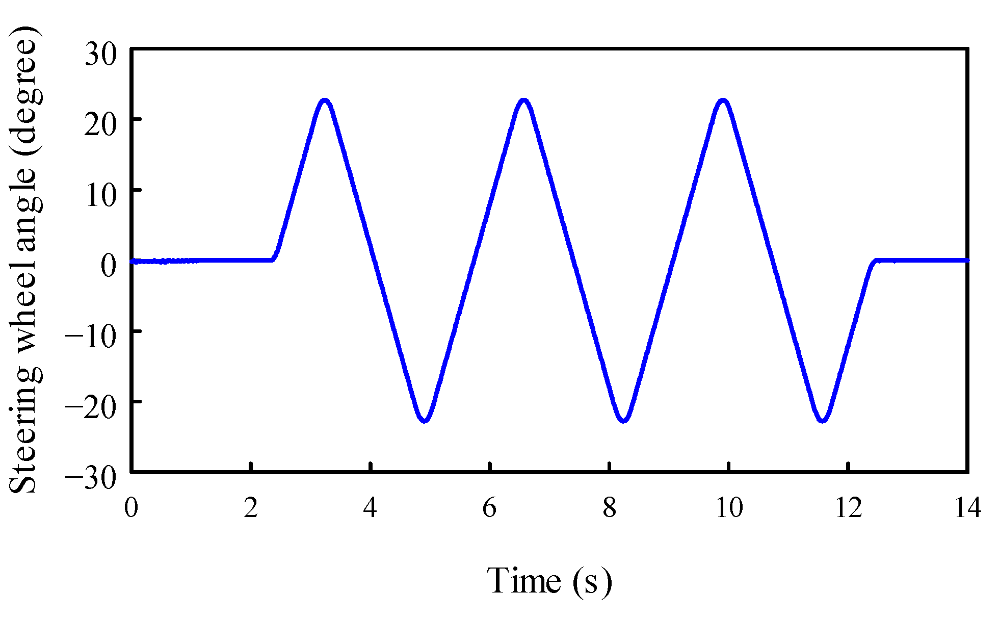
First, the suspension deformations were experimentally measured while performing the slalom test and compared with the deformations from the simulation using the dynamic model established in the previous section. For the slalom test, six cones were installed at equal intervals of 45 m on a flat road, and the test vehicle was driven zigzag between the cones at a constant speed of 100 km/h. The steering wheel angle variation for zigzag driving, as shown in Figure 5, was imposed on the vehicle. Note that the positive direction of the steering wheel angle is clockwise.

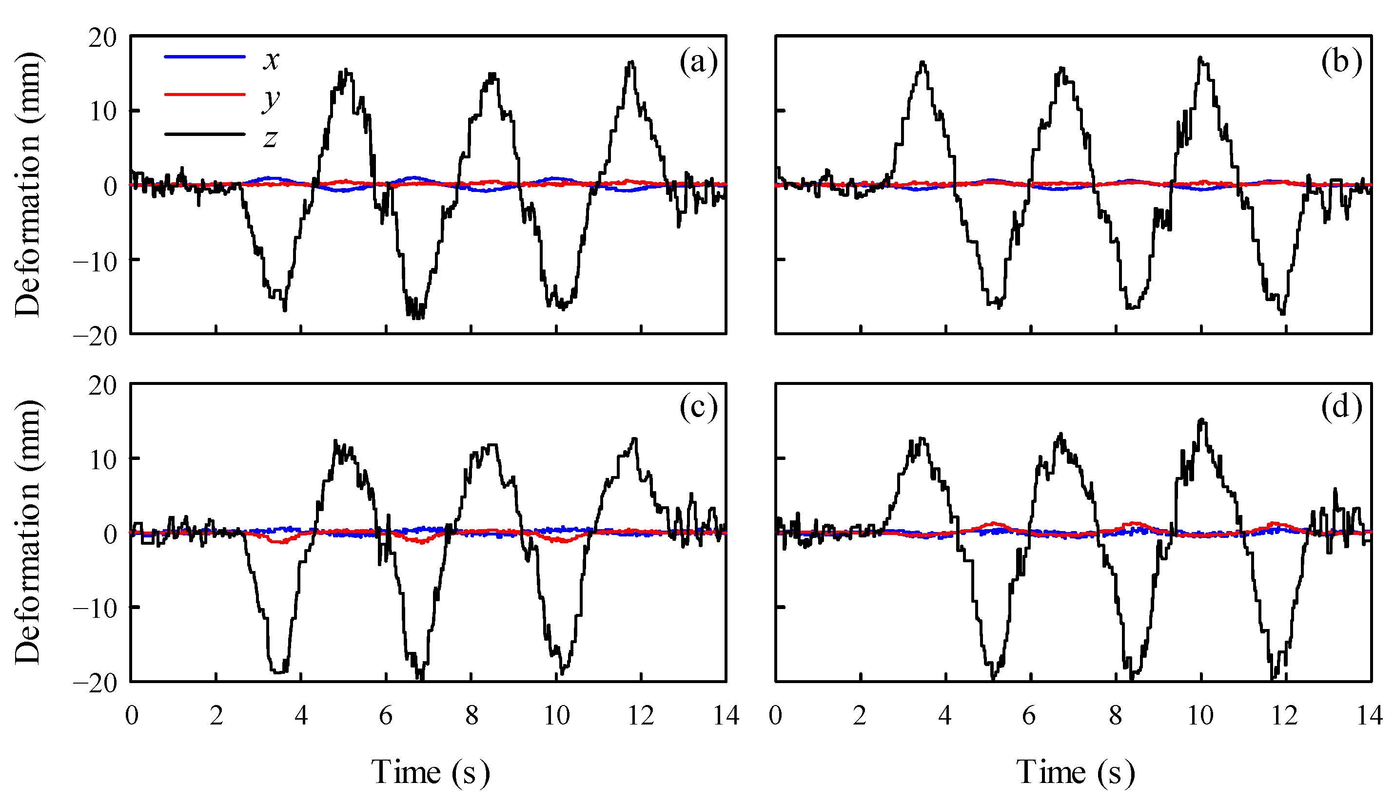
The suspension deformations measured during the slalom test are shown in Figure 6. Figure 6a shows the deformation at the left front wheel. Figure 6b shows the deformation at the right front wheel. Figure 6c shows the deformation at the left rear wheel. Figure 6d shows the deformation at the right rear wheel. In Figure 6, the blue, red, and black lines represent the deformations in the directions of the x, y, and z axes, respectively, which are the forward-rearward, left–right, and down–up directions with respect to the vehicle. The vertical deformations of the left suspensions of the vehicle (Figure 6a,c) have opposite phases to those of the right suspensions (Figure 6b,d). This is because the vehicle body rolls about the x-axis during turning, causing compressive deformation on the left side of the suspension and tensile deformation on the right side. The deformations in the z-direction are much larger than those in the x- and y-directions. This implies that the suspensions, which are connected in a nearly vertical position between the wheels and body, are vertically tensioned or compressed. Therefore, only the z-directional suspension deformations were considered in the comparison between the simulation and experimental results.

Simulations were performed with the dynamic vehicle model expressed as the equations of motion derived in the previous section. After obtaining the roll moment $M_r$ using the centrifugal force computed with the steering wheel angle for the slalom test shown in Figure 5, it was substituted into the equations of motion given by Equation (19). Applying the Newmark time integration method [36] with a time step size of 0.005 s to the equations of motion, the time histories of the bounce displacement ($Z$), pitch angle ($\phi$), roll angle ($\theta$), and vertical displacements of the unsprung masses ($z_1$, $z_2$, $z_3$, $z_4$) were computed. Using these time histories, the vertical suspension deformations at the four wheels were computed from the following linearized deformations:

$$\begin{gathered} d_1=Z-z_1-w_1\theta +l_1\phi , d_2=Z-z_2+w_2\theta +l_1\phi , \\ {d}_3=Z-z_3-w_1\theta -l_2\phi , d_4=Z-z_4+w_2\theta -l_2\phi \end{gathered}$$

(20)

The dynamic responses of the suspension deformations by simulation and experiment during the slalom test for 14 s are shown in Figure 7. Figure 7a represents the left front wheel; Figure 7b corresponds to the right front wheel; Figure 7c illustrates the left rear wheel; and Figure 7d depicts the right rear wheel. In Figure 7, the red and blue solid lines represent the simulated and experimental results, respectively. Figure 7 shows that the overall behaviors of the simulation are very similar to those of the experiment. This implies that the vehicle dynamics model presented in this study can be used to predict the behavior of a vehicle during a slalom test. However, the experimental results for the suspension deformations at all wheels had high-frequency vibrations compared with the simulation results. This is because, unlike the vehicle dynamic model, real vehicles have high-frequency components of vibration in suspension deformations. These high-frequency components are caused by wheel vibrations owing to the uneven road surface and the vibrations of various power transmission system components.

Next, while the steering wheel angle shown in Figure 8 was imposed on the vehicle, the suspension deformations were measured during the double lane change test. These measured deformations were compared with the simulated deformations to validate the vehicle dynamic model. The double-lane change test was performed by maintaining the vehicle speed constant at 100 km/h. Similar to the slalom test, the suspension deformations in the horizontal directions of the vehicle (x and y directions) were very small compared to the deformations in the vertical direction (the z direction). Therefore, the deformations in only the vertical direction were compared between the simulation and the experiment.

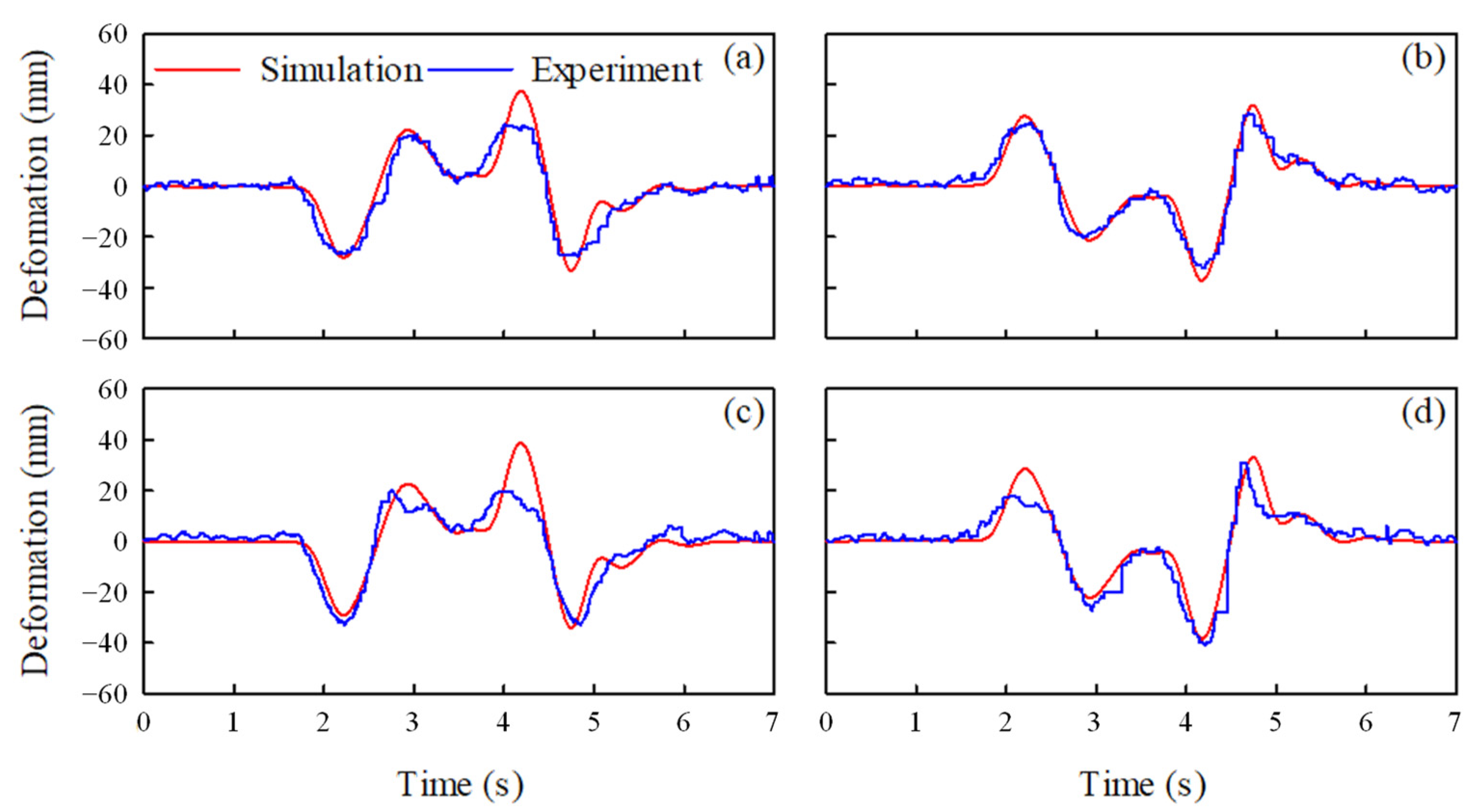
Figure 9 compares the results of the simulation and experiment for suspension deformations during the 7 s double lane change test. The suspension deformations at the four wheels are shown in Figure 9a–d, where the red and blue lines represent the simulation and experiment results, respectively. For the double-lane change test, the suspension deformations obtained by simulation using the vehicle dynamic model presented in this study followed the deformations measured through the experiment. However, slightly larger overshoots are observed in the simulation results compared to the experimental results at approximately 4.09 s in Figure 9a,c and 2.08 s in Figure 9d. This implies that the simplified and linearized vehicle dynamic model proposed in this study does not sufficiently reflect the complex kinematic and nonlinear elements of an actual vehicle. The numerical calculation errors may be attributable to the modeling of the nonlinear suspension system with variable stiffness and damping as a linear system. Nevertheless, the suggested model simulates the overall vehicle behavior relatively well while performing the double-lane change test.

Finally, the validity of the vehicle model was further confirmed through a step steer test. This involved comparing the suspension deformations measured on the actual vehicle in motion with the deformations calculated in the simulation using the presented model. The step steer test, often referred to as the J-turn test, involves applying a fast steering-wheel input to a fixed magnitude of the steering wheel angle while the vehicle moves along a straight path at a constant speed. While maintaining the vehicle speed at 100 km/h, the steering wheel angle, shown in Figure 10, was imposed on the vehicle.

The suspension deformations for the step steer test by simulation and measurement are shown in Figure 11. This figure shows that the suspension deformations obtained by the simulation, indicated by the red line, were in good overall agreement with the deformations measured by the experiment, indicated by the blue line. The high-frequency components in the time responses of suspension deformations, which were shown in the experimental results of the slalom test above, were also observed in the experimental results of the step steer test. Consequently, the simulations using the vehicle dynamic model proposed in this study provide reasonable computations of the suspension deformations for the three tests: the slalom, double lane change, and step steer.

4. Results and Discussion

In this section, not only the natural frequencies and mode shapes of the dynamic vehicle model are analyzed, but the effects of suspension stiffness, suspension damping, and anti-roll bar torsional stiffness on the dynamic response of the vehicle are also analyzed. The natural frequencies, mode-shaped responses, and dynamic responses were computed using MATLAB [37], which is a programming and numeric computing platform.

4.1. Natural Frequencies and Mode Shapes

Considering the natural frequencies and mode shapes of the vehicle model developed in Section 2, the natural frequency and mode shape were computed from the eigenvalue problem obtained by ignoring the damping term on the left and the force term on the right in Equation (19). As the damping properties have little influence on the natural frequencies, the damping term is negligible. Assuming $q=Q{\mathrm{e}}^{\mathrm{j}\omega t}$ where $\mathrm{j}=\sqrt{-1}$, $\omega$ is the natural frequency, and $Q$ is the modal vector, the eigenvalue problem is given by

$$(K-{\omega }^2\mathbf{M})\mathbf{Q}=\mathbf{0}$$

(21)

As the proposed model has seven degrees of freedom, the number of acquired natural frequencies and corresponding mode shapes is seven. The computed natural frequencies are 1.44, 1.62, 1.99, 12.73, 13.78, 15.45, and 16.67 Hz. The obtained mode shapes for these natural frequencies are displayed in Figure 12 and Figure 13, which show the mode shapes for the sprung and unsprung masses, respectively. In these figures, the dashed lines represent the positions where each mass does not move, and the solid lines represent the mode shapes where each mass moves.

The mode shapes of the sprung mass are shown in Figure 12. The bounce mode is for a vertical motion of the sprung mass, the pitch is for a rotation about the $y$ axis, and the roll mode is for a rotation about the $x$ axis. However, because the two modes shown in Figure 12a,b are modes in which bounce and pitch motions are combined, it is difficult to clearly distinguish these two modes as the bounce and pitch modes. In the mode shown in Figure 12a, bounce motion is more dominant than pitch motion. In contrast, the mode shown in Figure 12b has more pitch motion than bounce motion. In this study, the two modes with combined bounce and pitch motions, shown in Figure 12a,b, are called bounce–pitch modes. Comparing Figure 12a,b, the mode in Figure 12c has a distinct roll motion, indicating that it is a roll mode. The natural frequencies for the bounce–pitch modes are 1.44 and 1.62 Hz, and the natural frequency for the roll mode is 1.99 Hz.

The mode shapes of the unsprung masses are displayed in Figure 13, where Figure 13a–d show the in-phase front wheel mode, out-of-phase front wheel mode, in-phase rear wheel mode, and out-of-phase rear wheel mode, respectively. In the in-phase front wheel mode with a natural frequency of 12.73 Hz, the two front wheels vibrate in the same direction, but the rear wheels are motionless (Figure 13a). On the other hand, the out-of-phase front wheel mode with a natural frequency of 13.78 Hz has vibrations of the front wheels in opposite directions and no motion in the rear wheels (Figure 13b). Similarly, in the in-phase rear wheel mode with a natural frequency of 15.42 Hz, the rear wheels vibrate in the same direction (Figure 13c). Additionally, in the out-of-phase rear wheel mode with a natural frequency of 16.67 Hz, the rear wheels vibrate in opposite directions (Figure 13d). Note that the natural frequencies of the vibration modes related to sprung masses are much lower than those of the vibration modes related to unsprung masses.

We analyzed the effects of the vehicle suspension stiffness and anti-roll bar torsional stiffness on the natural frequencies for the sprung and unsprung modes. The natural frequencies for the change in stiffness are shown in Figure 14, Figure 15, Figure 16, Figure 17, Figure 18 and Figure 19, where the abscissa represents the front suspension stiffness and the ordinate represents the natural frequency. The numbers on the abscissa indicate the multiples of the stiffness given in Section 2. For example, “0.1” on the abscissa of Figure 14 means 0.1 times $k_f$, which is the front suspension stiffness of $0.1k_f$. In Figure 14, Figure 15, Figure 16, Figure 17, Figure 18 and Figure 19, the hollow inverted triangles represent the natural frequencies of the two bounce–pitch modes of the sprung mass. These inverted triangles are not connected by lines because the bounce and pitch modes are not clearly distinguished and are mixed, as previously explained. The natural frequencies for the roll mode of the sprung mass are shown as blue triangles connected by solid blue lines. The natural frequencies for the in-phase front wheel mode, out-of-phase front wheel mode, in-phase rear wheel mode, and out-of-phase rear wheel mode are represented by hollow squares with solid lines, hollow circles with red dotted lines, hollow triangles with solid lines, and blue crosses with blue dotted lines, respectively.

First, we consider the effect of suspension stiffness variation on the natural frequencies of the modes. Figure 14 shows the natural frequencies for the values of the front suspension stiffness, $0.01k_f$, $0.1k_f$, $k_f$, $10k_f$, and $100k_f$, where $k_f=44,400$ N/m, as given in Section 2. The dimensions and material properties of the vehicle model, excluding the front suspension stiffness, were the same as those presented in Section 2. As shown in the figure, the natural frequencies of the sprung mass modes were much lower than those of the unsprung mass modes. The natural frequencies for the bounce–pitch modes of the sprung mass are 0.16 and 1.61 Hz for $0.01k_f$, 0.49 and 1.61 Hz for $0.1k_f$, 1.44 and 1.62 Hz for $k_f$, 1.61 and 2.95 Hz for $10k_f$, and 1.62 and 3.51 Hz for $100k_f$. Notably, one of the natural frequencies for the bounce–pitch modes does not change significantly and remains close to 1.61 Hz. Other natural frequencies not close to 1.61 Hz increase to 0.16, 0.49, 1.44, 2.95, and 3.51 Hz as the suspension stiffness increases. As observed in this figure, the natural frequencies for the roll mode of the sprung mass, as well as the in-phase and out-of-phase front wheel modes, increase with the front suspension stiffness. However, the natural frequencies of the in-plane and out-of-plane rear-wheel modes remained constant even as the front suspension stiffness increased. In other words, the front suspension stiffness affects the natural frequencies of the front-wheel modes but not the frequencies of the rear-wheel modes.

The changes in the natural frequencies of the dynamic vehicle model are presented in Figure 15 when the rear suspension stiffness is varied from $0.01k_r$ to $100k_r$ while the front suspension stiffness is fixed at $k_f$. Similar to Figure 14, one of the natural frequencies for the bounce–pitch modes increases and the others remain constant at around 1.45 Hz as the rear suspension stiffness increases. The natural frequency for the roll mode also increased with the rear suspension stiffness. However, when the rear suspension stiffness increases, the natural frequencies of the rear wheel modes increase, while the natural frequencies of the front wheel modes remain constant. Based on the analysis of Figure 14 and Figure 15, it can be inferred that an increase in either the front and rear wheel suspension stiffnesses leads to an increase in the natural frequencies associated with the roll mode, wheel modes, and one of the bounce–pitch modes. However, the frequencies of the other modes remain constant. Figure 16 shows the changes in natural frequencies when the stiffnesses of both the front and rear suspensions increase simultaneously from 0.01 times to 100 times the stiffness values given in Section 2. In this case, as expected, the natural frequencies for all modes for the sprung and unsprung masses increased.

Next, we analyzed the effects of changes in the torsional stiffness of the front anti-roll bar on the natural frequencies of the vehicle model. Using the torsional stiffness of the front anti-roll bar ${\kappa }_f=62,085$ N·m/rad as a reference value, the natural frequencies were computed for five torsional stiffness values of 0.01, 0.1, 1, 10, and 100 times ${\kappa }_f$. The computed results are shown in Figure 17. As shown in this figure, the natural frequency for the roll mode of the sprung mass increases with the torsional stiffness of the front anti-roll bar. However, the natural frequencies for the bounce–pitch modes remain unchanged, regardless of the torsional stiffness. Among the natural frequencies for the modes of unsprung masses, only the natural frequency for the out-of-phase front wheel mode increases with the torsional stiffness, while the natural frequencies of other modes remain unchanged.

Figure 18 shows the change in the natural frequencies of the dynamic vehicle model when the torsional stiffness of the rear anti-roll bar is increased. The natural frequencies were computed while increasing the torsional stiffness of the rear anti-roll bar from $0.01{\kappa }_r$ to $100{\kappa }_r$ with all other dimensions and material properties fixed. The value of ${\kappa }_r$ is 58,098 N·m/rad, as given in Section 2. As shown in Figure 18, the natural frequencies of the sprung mass roll mode and out-of-phase rear wheel mode increased with the torsional stiffness of the rear anti-roll bar. However, this change in torsional stiffness had no effect on the natural frequencies of the other modes. It is observed from Figure 17 and Figure 18 that if only one of the two anti-roll bar torsional stiffnesses increases, the natural frequencies of the roll mode and the corresponding out-of-phase wheel mode increase, while the natural frequencies of the other modes remain unchanged.

Figure 19 shows the changes in natural frequencies of the vehicle model when the torsional stiffnesses of the front and rear anti-roll bars increased simultaneously. The natural frequencies in this figure were computed with values of 0.01, 0.1, 1, 10, and 100 times the values of ${\kappa }_f$ and ${\kappa }_r$ presented in Section 2. As shown in this figure, the natural frequencies of the bounce–pitch modes and in-phase wheel modes remain unchanged even when the torsional stiffness increases. However, the natural frequencies of the roll mode and out-of-phase wheel modes increase with torsional stiffness. Comparing Figure 17, Figure 18 and Figure 19, the result of simultaneously increasing the front and rear torsional stiffnesses (Figure 19) is a combination of the results of increasing the front torsional stiffness (Figure 17) and rear torsional stiffness (Figure 18). Therefore, the natural frequency of the roll mode in Figure 19 is higher than the natural frequencies of the roll modes shown in Figure 17 and Figure 18.

4.2. Dynamic Responses

We analyzed the effects of changes in the design parameters on the dynamic response of the vehicle model. In this study, suspension stiffness, suspension damping, and anti-roll bar torsional stiffness, which are relatively easy to change, were selected as the design parameters related to dynamic responses. The sprung mass, mass moment of inertia for the sprung mass, unsprung mass, and tire stiffness are not considered design parameters because their design changes are difficult. To obtain the dynamic responses of the vehicle model, simulations were performed for the step steer test with the steering wheel angle shown in Figure 10 and a vehicle speed of 100 km/h. The reason for selecting dynamic responses for the step steer test is that the step steer test provides a much harsher driving condition than the slalom and double-lane tests. Therefore, the dynamic responses to the step steer test have been analyzed in many studies [38,39,40]. When the step steer test is performed, the dynamic response to the pitch angle is much smaller than the dynamic response to the bounce displacement and roll angle. Therefore, in this study, the dynamic responses for the bounce and roll, excluding the pitch, are analyzed.

First, the effects of suspension stiffness on the dynamic response of the sprung mass’s bounce and roll were investigated. The dynamic responses of the bounce displacement and roll angle for the step steer test are shown in Figure 20. These responses were computed for the three sets of front and rear suspension stiffnesses: ($0.1k_f$, $0.1k_r$), ($k_f$, $k_r$), and ($10k_f$, $10k_r$), where the values of $k_f$ and $k_r$ are the same as those presented in Section 2.

As shown in Figure 20a, a positive bounce displacement occurs when the steering wheel angle of Figure 10 is given to the vehicle model. As shown in this figure, the bounce displacement is large when the suspension stiffness is low (in the case of $0.1k_f$ and $0.1k_r$) and is small when the stiffness is high (in the case of $10k_f$ and $10k_r$). However, Figure 20b shows that the roll angles obtained by this step steer test have negative values and become larger as the suspension stiffness decreases. The negative roll angle was caused because a positive steering wheel angle moved the left side of the sprung mass down and the right side up, as shown in Figure 11, resulting in a negative roll angle. Notably, the bounce displacement and roll angle, shown as solid black lines, exhibit high-frequency oscillations when the suspension stiffness is large. The high-frequency oscillation period of the bounce displacement was approximately 0.292 s, and the oscillation period of the roll angle was approximately 0.250 s. These periods correspond to frequencies of 3.42 and 4.00 Hz. The natural frequencies of the bounce–pitch modes are 2.93 and 3.46 Hz, and the natural frequency of the roll mode is 3.96 Hz when the front and rear suspension stiffness are $10k_f$ and $10k_r$, respectively. Considering these natural frequencies, the oscillation of 3.42 Hz in the bounce displacement is due to the bounce–pitch mode with 3.46 Hz, while the oscillation of 4.00 Hz in the roll angle is due to the roll mode with 3.96 Hz.

The oscillation amplitudes of the bounce acceleration are shown in Figure 21a. Additionally, the roll angular acceleration shown in Figure 21b increases with suspension stiffness. The oscillation frequencies for these accelerations are the same as those for the displacements in Figure 20. As mentioned above, these oscillations occur due to the natural vibrations of the bounce–pitch and roll modes. The increase in the acceleration values of the bounce and roll may adversely affect the riding comfort and steering stability that passengers can feel.

Next, we analyze the effects of suspension damping on the dynamic responses to the bounce and roll motions of the sprung mass. Based on the damping values $c_f$ and $c_r$ of the front and rear suspensions presented in Section 2, the dynamic responses of the vehicle were calculated for three damping values of 0.5, 1, and 1.5 times these values. Damping values of 0.1, 1, and 10 times $c_f$ and $c_r$ were not used because the vehicle system with $10c_f$ and $10c_r$ showed unrealistically overdamped motion. Figure 22 shows displacements for three damping values of 0.1, 1, and 10 times $c_f$ and $c_r$, demonstrates that the oscillation amplitudes of the bounce displacement and roll angle decrease as damping increases. This phenomenon is also observed in Figure 23, which shows the bounce acceleration and roll angular acceleration. It is widely recognized that suspension damping contributes to reducing the dynamic responses of the vehicle. Therefore, it improves the ride comfort and cornering feel of the vehicle.

Finally, the effects of the torsional stiffness of the anti-roll bar on the dynamic responses to the bounce and roll motions are considered. Based on the torsional stiffness ${\kappa }_f$ and ${\kappa }_r$ of the front and rear anti-roll bars presented in Section 2, simulations for the step steer test were performed for the three torsional stiffness values of 0.1, 1, and 10 times ${\kappa }_f$ and ${\kappa }_r$. The dynamic responses of the bounce displacements and roll angles for these three torsional stiffness values are shown in Figure 24. This figure illustrates that the larger the torsional stiffness, the smaller not only the bounce displacement and roll angle but also their oscillation amplitudes. Figure 25 also shows that the amplitudes of the bounce acceleration and roll angular acceleration decrease as the torsional stiffness increases. Consequently, as shown in Figure 24 and Figure 25, the increase in the torsional stiffness of the anti-roll bar provides a more comfortable driving environment for the driver by reducing the roll and bounce motions.

Automobile manufacturers utilize the Dynamic Kinematics and Compliance (K&C) System to evaluate the ride and handling performance of their vehicles. By analyzing the kinematic characteristics of suspension and the compliance characteristics of springs and bushings, these test devices can help simulate a vehicle’s dynamic state while running on a real road indoors. To achieve this, a dependable and controllable vehicle model is necessary, and the model developed in this study can be applied for this purpose.

5. Summary and Conclusions

This study presents a dynamic vehicle model that can analyze the dynamic behavior of a vehicle without an actual driving test. Considering the centrifugal force acting on the vehicle during turning and the torsional stiffness of the anti-roll bar, a vehicle model with seven degrees of freedom was constructed to investigate the dynamic characteristics and responses to driving conditions. The equations of motion for this vehicle model were derived using Lagrange’s equation. The constructed vehicle model was verified by comparing the suspension deformations computed by the simulations with the deformations measured through actual driving tests. Using this model, the natural frequencies and mode shapes of the vehicles were analyzed. Moreover, the effects of the suspension stiffness and anti-roll bar torsional stiffness on the natural frequencies were also analyzed. In addition, the effects of suspension stiffnesses, suspension damping coefficients, and anti-roll bar torsional stiffnesses on the dynamic responses of the vehicle were also investigated when the vehicle was under the step steer test. The results obtained in this study can be applied not only to internal combustion engine vehicles but also to electric and hybrid vehicles.

The results of analyzing the dynamic characteristics of the driving vehicle using the proposed dynamic model are summarized as follows:

• The natural frequencies of the vibration modes associated with the sprung mass were much lower than those of the modes associated with the unsprung masses.
• When one of the front and rear wheel suspension stiffnesses increases, the natural frequencies for the roll mode, the associated wheel modes, and one of the bounce–pitch modes increase, whereas the frequencies of the other modes remain constant.
• When both the front- and rear-wheel suspension stiffnesses increase simultaneously, the natural frequencies of all modes for the sprung and unsprung masses increase.
• When only one of the two anti-roll bars’ torsional stiffnesses increases, the natural frequencies of the roll mode and the corresponding out-of-phase wheel mode increase, while the natural frequencies of the other modes remain unchanged.
• When the two torsional stiffnesses of the front and rear anti-roll bars increase simultaneously, the natural frequencies of the roll mode and out-of-phase wheel modes increase, while those of the bounce–pitch modes and the in-phase wheel modes remain unchanged.

When performing the step steer test, the analysis results of the effects of design parameters such as suspension stiffness, suspension damping, and anti-roll bar torsional stiffness on the dynamic responses of the vehicle model are as follows:

• The bounce displacement and roll angle decrease with the suspension stiffness.
• When the suspension stiffness is large, the bounce displacement and roll angle have high-frequency oscillations because of the bounce–pitch mode and the roll mode, respectively.
• The oscillation amplitudes in the bounce acceleration and roll angular acceleration increase with the suspension stiffness.
• Suspension damping contributes to reducing the dynamic responses of the vehicle, including both the displacements and accelerations for bounce and roll motions.
• The torsional stiffness of the anti-roll bar reduced both the displacements and accelerations of the bounce and roll motions.

References

1. Genta, G. Motor Vehicle Dynamics: Modeling and Simulation; World Scientific: Singapore, 1997. [Google Scholar]
2. Gillespie, T.D. Fundamentals of Vehicle Dynamics; Society of Automotive Engineers, Inc.: Warrendale, PA, USA, 2000. [Google Scholar]
3. Gillespie, T.D.; Karamihas, S.M. Simplified models for truck dynamic response to road inputs. Int. J. Heavy Veh. Syst. 2000, 7, 52–63. [Google Scholar] [CrossRef]
4. Pacejka, H.B.; Bakker, E. The magic formula tyre model. Veh. Syst. Dyn. 1992, 21, 1–18. [Google Scholar] [CrossRef]
5. Dixon, J.C. The Shock Absorber Handbook; John Wiley & Sons: Hoboken, NJ, USA, 2008. [Google Scholar]
6. Choi, S.B.; Lee, H.K.; Chang, E.G. Field test results of a semi-active ER suspension system associated with skyhook controller. Mechatronics 2001, 11, 345–353. [Google Scholar] [CrossRef]
7. Jonsson, P.; Johansson, O. Prediction of vehicle discomfort from transient vibrations. J. Sound Vib. 2005, 282, 1043–1064. [Google Scholar] [CrossRef]
8. Uys, P.E.; Els, P.S.; Thoresson, M.J. Criteria for handling measurement. J. Terramech. 2006, 43, 43–67. [Google Scholar] [CrossRef]
9. Darling, J.; Hickson, L.R. An Experimental Study of a Prototype Active Anti-Roll Suspension System. Veh. Syst. Dyn. 1998, 29, 309–329. [Google Scholar] [CrossRef]
10. Choi, S.B.; Han, Y.M.; Song, H.J.; Sohn, J.W.; Choi, H.J. Field test on vibration control of vehicle suspension system featuring ER shock absorbers. J. Intell. Mater. Syst. Struct. 2007, 18, 1169–1174. [Google Scholar] [CrossRef]
11. Sun, T.; Zhang, Y.; Barak, P. Quarter Vehicle Ride Model. SAE Pap. Ser. 2002, 1, 1581. [Google Scholar]
12. Georgiou, G.; Verros, G.; Natsiavas, S. Multi-objective optimization of quarter-car models with a passive or semi-active suspension system. Veh. Syst. Dyn. 2007, 45, 77–92. [Google Scholar] [CrossRef]
13. Singh, D.; Aggarwal, M.L. Passenger seat vibration control of a semi-active quarter car system with hybrid Fuzzy-PID approach. Int. J. Dyn. Control. 2015, 5, 287–296. [Google Scholar] [CrossRef]
14. Singh, D. Ride comfort analysis of passenger body biodynamics in active quarter car model using adaptive neuro-fuzzy inference system based super twisting sliding mode control. J. Vib. Control. 2019, 25, 1866–1882. [Google Scholar] [CrossRef]
15. Sun, T.; Zhang, Y.; Barak, P. 4-DOF Vehicle Ride Model. SAE Pap. Ser. 2002, 1, 1580. [Google Scholar]
16. Zhu, H.; Yang, J.; Zhang, Y. Modeling and optimization for pneumatically pitch-interconnected suspension of a vehicle. J. Sound Vib. 2018, 432, 290–309. [Google Scholar] [CrossRef]
17. Hudha, K.; Jamaludding, H.; Samin, P.M.; Rahman, R.A. Semi Active Roll Control Suspension (SARCS) System on a New Modified Half Car Model. SAE Pap. Ser. 2003, 1, 2274. [Google Scholar]
18. Gosselin-Brisson, S.; Bouazara, M.; Richard, M.J. Design of an active anti-roll bar for off-road vehicles. Shock Vib. 2019, 16, 155–174. [Google Scholar] [CrossRef]
19. Abu Barak, S.A.; Samin, P.M.; Azhar, A.A. Modelling and Validation of Vehicle Ride Comfort Model. Appl. Mech. Mater. 2014, 554, 515–519. [Google Scholar] [CrossRef]
20. Palli, S.; Sharma, R.C.; Rao, P.P.D. Dynamic Behaviour of a 7 DoF Passenger Car Model. Int. J. Veh. Struct. Syst. 2017, 9, 57–63. [Google Scholar]
21. Senthilkumar, P.; Sivakumar, K.; Kanagarajan, R.; Kuberan, S. Fuzzy Control of Active Suspension System using Full Car Model. Mechanika 2018, 24, 240–247. [Google Scholar] [CrossRef]
22. Ghike, C.; Shim, T. 14 Degree-of-Freedom Vehicle Model for Roll Dynamics Study. SAE Pap. Ser. 2006, 1, 1277. [Google Scholar]
23. ANSYS-Motion 2019; ANSYS Inc.: Canonsburg, PA, USA, 2019.
24. RecurDyne 8.3; RecurDyne, Inc.: Palo Alto, CA, USA, 2020.
25. MSC/Adams 2019; MSC Software Corporation: Santa Ana, CA, USA, 2019.
26. Simpack 9.9; MSC Software Corporation: Santa Ana, CA, USA, 2019.
27. Julio-Rodríguez, J.d.C.; Santana-Díaz, A.; Ramirez-Mendoza, R.A. Individual Drive-Wheel Energy Management for Rear-Traction Electric Vehicles with In-Wheel Motors. Appl. Sci. 2021, 11, 4679. [Google Scholar] [CrossRef]
28. Trzesniowski, M. Steering Kinematics; Harrer, M., Pfeffer, P., Eds.; Springer International Publishing: Cham, Switzerland, 2017; pp. 398–402. [Google Scholar]
29. Cong, S.; Shangbin, S.; Zan, L. Vehicle roll stability analysis considering lateral-load transfer rate. In Proceedings of the International Conference on Transportation Information and Safety (ICTIS) 2015, Wuhan, China, 25–28 June 2015; pp. 398–402. [Google Scholar]
30. Yoon, D.S.; Kim, G.W.; Choi, S.B. Response time of magnetorheological dampers to current inputs in a semi-active suspension system: Modeling, control and sensitivity analysis. Mech. Syst. Signal Proc. 2021, 146, 106999. [Google Scholar] [CrossRef]
31. Lajqi, S.; Gugler, J.; Lajqi, N.; Shala, A.; Likaj, R. Possible experimental method to determine the suspension parameters in a simplified model of a passenger car. Int. J. Automot. Technol. 2012, 13, 615–621. [Google Scholar] [CrossRef]
32. Taylor, R.; Bashford, L.; Schrock, M. Methods for measuring vertical tire stiffness. Trans. ASAE 2000, 43, 1415–1419. [Google Scholar] [CrossRef]
33. ISO 13674-1:2010; Road Vehicles—Test Method for the Quantification of on-Centre Handling—Part 1: Weave Test. International Organisation for Standardization (ISO): Geneva, Switzerland, 2010.
34. ISO 3888-1:2018; Passenger Cars—Test Track for a Severe Lane-Change Manoeuvre—Part 1: Double Lane-Change. International Organisation for Standardization (ISO): Geneva, Switzerland, 2018.
35. ISO 7401:2003; Road Vehicles—Lateral transient response test methods-Open-loop test methods. International Organisation for Standardization (ISO): Geneva, Switzerland, 2003.
36. Newmark, N.M. A method of computation for structural dynamics. J. Engrg. Mech. Div. 1959, 85, 67–94. [Google Scholar] [CrossRef]
37. MATLAB R2020a; MathWorks: Natick, MA, USA, 2020.
38. Sorniotti, A.; D’Alfio, N. Vehicle Dynamics Simulation to Develop an Active Roll Control System. In SAE Technical Paper; No. 2007-01-0828; SAE International: Warrendale, PA, USA, 2007. [Google Scholar]
39. Zhang, J.; Wang, M. Integrated Adaptive Steering Stability Control for Ground Vehicle with Actuator Saturations. Appl. Sci. 2022, 12, 8502. [Google Scholar] [CrossRef]
40. Chen, H.; Gong, M.-D.; Zhao, D.-X.; Liu, W.-B.; Jia, G.-Y. Coordination Control of Multi-Axis Steering and Active Suspension System for High-Mobility Emergency Rescue Vehicles. Mathematics 2022, 10, 3562. [Google Scholar] [CrossRef]
Figure 1. Ackermann steering geometry for the front steer angles of the inner and outer wheels.
Applsci 13 05903 g001
Figure 2. Dynamic model of a vehicle with seven degrees of freedom.
Applsci 13 05903 g002
Figure 3. Front view of the dynamic model of the vehicle.
Applsci 13 05903 g003
Figure 4. Schematic diagram for the experimental setup for measuring suspension deformations.
Applsci 13 05903 g004
Figure 5. Time variation of the steering wheel angle for the slalom test.
Applsci 13 05903 g005
Figure 6. Suspension deformations measured during the slalom test: (a) at the left front wheel; (b) at the right front wheel; (c) at the left rear wheel; and (d) at the right rear wheel.
Applsci 13 05903 g006
Figure 7. Comparison of the vertical suspension deformations during the slalom test between the simulation and experiment: (a) at the left front wheel; (b) at the right front wheel; (c) at the left rear wheel; and (d) at the right rear wheel.
Applsci 13 05903 g007
Figure 8. Time variation of the steering wheel angle for the double lane change test.
Applsci 13 05903 g008
Figure 9. Comparison of the vertical suspension deformations during the double lane change test between the simulation and experiment: (a) at the left front wheel; (b) at the right front wheel; (c) at the left rear wheel; and (d) at the right rear wheel.
Applsci 13 05903 g009
Figure 10. Time variation of the steering wheel angle for the step steer test.
Applsci 13 05903 g010
Figure 11. Comparison of the vertical suspension deformations during the step steer test between the simulation and experiment: (a) at the left front wheel; (b) at the right front wheel; (c) at the left rear wheel; and (d) at the right rear wheel.
Applsci 13 05903 g011
Figure 12. Mode shapes of the sprung mass: (a) the bounce–pitch mode with the natural frequency of 1.44 Hz; (b) the bounce–pitch mode with the natural frequency of 1.62 Hz; and (c) the roll mode with the natural frequency of 1.99 Hz.
Applsci 13 05903 g012
Figure 13. Mode shapes of the unsprung mass: (a) the in-phase front wheel mode (12.73 Hz); (b) the out-of-phase front wheel mode (13.78 Hz); (c) the in-phase rear wheel mode (15.45 Hz); and (d) the out-of-phase rear wheel mode.
Applsci 13 05903 g013
Figure 14. Natural frequencies for the variation of the front suspension stiffness.
Applsci 13 05903 g014
Figure 15. Natural frequencies for the variation of the rear suspension stiffness.
Applsci 13 05903 g015
Figure 16. Natural frequencies when the front and rear suspension stiffnesses change simultaneously.
Applsci 13 05903 g016
Figure 17. Natural frequencies for the variation of the torsional stiffness of the front anti-roll bar.
Applsci 13 05903 g017
Figure 18. Natural frequencies for the variation of the torsional stiffness of the rear anti-roll bar.
Applsci 13 05903 g018
Figure 19. Natural frequencies when the torsional stiffnesses of the front and rear anti-roll bars change simultaneously.
Applsci 13 05903 g019
Figure 20. Dynamic responses of the displacements for three values of the suspension stiffness: (a) the bounce and (b) the roll.
Applsci 13 05903 g020
Figure 21. Dynamic responses of the accelerations for three values of the suspension stiffness: (a) the bounce and (b) the roll.
Applsci 13 05903 g021
Figure 22. Dynamic responses of the displacements for three values of the suspension damping: (a) the bounce and (b) the roll.
Applsci 13 05903 g022
Figure 23. Dynamic responses of the accelerations for three values of the suspension damping: (a) the bounce and (b) the roll.
Applsci 13 05903 g023
Figure 24. Dynamic responses of the displacements for three values of the torsional stiffness of the anti-roll bar: (a) the bounce and (b) the roll.
Applsci 13 05903 g024
Figure 25. Dynamic responses of the accelerations for three values of the torsional stiffness of the anti-roll bar: (a) the bounce and (b) the roll.
Applsci 13 05903 g025
Disclaimer/Publisher’s Note: The statements, opinions and data contained in all publications are solely those of the individual author(s) and contributor(s) and not of MDPI and/or the editor(s). MDPI and/or the editor(s) disclaim responsibility for any injury to people or property resulting from any ideas, methods, instructions or products referred to in the content.