Integrated Image Processing Toolset for Tracking Direction of Metal Grain Deformation

Abstract

Grain boundaries (GBs), which are among the mechanical properties of a material, are a microstructural aspect that contributes to the overall behavior of metal. A deep understanding of the behavior of the GBs’ deformation, dislocation, and fracture will encourage the rapid development of new materials and lead to the better operation and maintenance of materials during their designed lifetimes. In this study, an integrated image processing toolset is proposed to provide an expeditious approach to extracting GBs, tracking their location, and identifying their internal deformation. This toolset consists of three integrated algorithms: image stitching, grain matching, and boundary extraction. The algorithms are designed to simultaneously integrate high and low spatial resolution images for gathering high-precision boundary coordinates and effectively reconstructing a view of the entire material surface for the tracing of the grain location. This significantly reduces the time needed to acquire the dataset owing to the ability of the low spatial resolution lens to capture wider areas as the base image. The high spatial resolution lens compensates for any weakness of the base image by capturing views of specific sections, thereby increasing the observation flexibility. One application successfully described in this paper is tracking the direction of the metal grain deformation in global coordinates by stacking a specific grain before and after the deformation. This allows observers to calculate the direction of the grain deformation by comparing the overlapping areas after the material experiences a load. Ultimately, this toolset is expected to lead to further applications in terms of observing fascinating phenomena in materials science and engineering.

1. Introduction

Rapid developments in construction, future power generation, and transportation technology demand better materials to improve the integrity and safety of engineering systems [1]. In this regard, the metallography approach has helped researchers understand a material’s behavior such as the composition, amorphization, work hardening, heat treatment, and fracture toughness [2,3,4,5,6] from a microstructural point of view [2,3]. Understanding these microstructural aspects of a material’s behavior can be beneficial for preventing the material fracture caused by fatigue, creep, and an external force impact [7,8]. Tracking changes in the microstructure, including the grain boundary (GB) deformation, dislocation, and structural evolution, is essential because these problems contribute to the overall behavior of the metal [9,10,11,12,13]. In addition, it has been found experimentally that a significant reduction in the grain size is associated with a lower material durability and damage resistance [14,15]. Therefore, an accurate and automatic method for tracking the collective microstructural changes that occur as a result of various external force impacts can substantially facilitate microstructural analysis and modeling, thus shortening the time to the development of new materials and leading to the better operation and maintenance of such materials during their service life [16,17,18].

The microstructure of a metal consists of aggregates of grains that have diverse crystallographic lattice orientations with respect to their nearest neighboring grains [19] and unique bimodal histogram distributions. The past several years have witnessed rapid progress in investigating GB-mediated deformation using a variety of in situ and ex situ experimental techniques [20,21,22,23]. One rapid approach to extracting the metal GBs is accomplished via image processing and optical measurements. The edge-detection method is used to extract the GBs by detecting meaningful discontinuities in the pixel intensity values [24]. Several edge-detection methods have been proposed in the literature, but they are generally grouped into Gradient and Laplacian approaches [25,26,27]. These edge-detection approaches provide various levels of sophistication and computational efficiency by reducing the amount of data required and filtering out the useless features while preserving information regarding the significant structural properties of the GBs [28]. Implementing image binarization before the edge-detection algorithm provides a robust tracking ability with low storage requirements and straightforward processing compared to tracking discontinuous values on gray-level images [29,30]. Many researchers agree that the combination of image pre-processing approaches and image binarization enhances the clarity of an image, thus providing flexible methods for extracting the GBs [26]. Figure 1 shows a comparison of the edge detection on gray-level and binary images using gradient and Laplacian filters. Image binarization is an image transformation algorithm used to transform a grayscale image into a bi-level intensity image by converting any existing gradation [26]. Although binary images consist of significantly fewer intensity parameters than their counterparts, such as grayscale and sRGB images, they are more effective in terms of conceiving the shape and size of the object with significantly fewer computational processes, which is very beneficial for object recognition [31]. The algorithm separates the 0–255 image pixel intensity into a dual collective pixel intensity representing black and white colors. Image binarization works in a manner similar to that of a filter by transforming the unsuitable intensity matrix value of the pixel using a specific threshold separator [32]. The main focus of researchers is thus to improve the accuracy and reliability of the threshold separator, thus reducing the structural degradation of the image’s parts [26,27]. Experiments have shown that a uniform threshold value for the entire image dataset makes the extraction process suboptimal, owing to the changes in lamination and the poor image quality, especially at the edges [30,32]. In the case of extracting a metallographic image of a metal polycrystalline, the careless implementation of a threshold separator can eliminate the essential features of the grain, thus reducing the extraction accuracy of the GB. Unfortunately, the toolsets for automatically adjusting the thresholding are lacking, making the extraction process of GB unreliable.

In addition to extracting the GBs, the initial and final positions of the metal grain after the deformation must be recognized to track the grain deformation. This is essential because it has been found experimentally that, owing to the high spatial resolution of the optical microscopy used during the data acquisition, any positional error potentially reduces the precision of the final desired result [33]. Several methods have been proposed to address these issues. For example, Iwaszenko et al. (2013) proposed a GB segmentation technique for the polycrystalline images acquired under ambient light conditions with small inconsistencies in the light source reflectance [34]. The combination of an sRGB-to-gray-level image converter and a Gaussian filter (σ = 30) was utilized to increase the dataset clarity, after which an expert manually drew the boundaries of the grain on each ground-truth. This method successfully solves typical optical micrograph problems, including the lack of optical contrast, which occurs when adjusting the random parameter to achieve a clear grain image. Unfortunately, manually segmenting and stitching the grain section images requires a significant amount of time, and it is strongly dependent on the concentration of the expert. In the case of GB segmentation, Panda et al. (2019) proposed a deep-learning approach for segmenting plain microstructure images using generative adversarial networks (GANs) [35]. The dataset was prepared using an image binarization process with a global threshold (50–110) depending on the original image’s intensity. The proposed model can efficiently detect very thin edges in the vicinity of other thin edges. Again, it was found that global thresholding must be addressed to prevent erosion followed by dilation, which causes edge uniformity [36]. In addition, manual stitching can be improved by utilizing an image-stitching algorithm to improve the join quality with a quantifiable performance. The image-stitching algorithm is performed by using feature detectors (FDs) [37], which track the key points in two or more frames and match pixels based on their value and physical proximity [38,39,40,41,42,43]. Achievements in GB tracking are progressing rapidly for in situ atomic-resolution experiments [44]. Despite the extensive implementation of image-processing algorithms for grain boundary tracking, several issues regarding the user flexibility and training time remain unresolved [45]. Still, it has been found that the application of FDs to image processing using a binary image gave a faster tracking performance while using fewer computational resources [46,47]. This is essential because similarity tracking, segmenting, and stitching high spatial resolution images require efficient FDs to significantly reduce the training time.

From the above discussion, two issues need to be addressed: (1) improving the threshold separator for the image binarization process and (2) developing an integrated and flexible image-processing method for tracking the metal grain deformation. The development of a threshold adjustment tool set that allows observers to adapt threshold separators using the unique properties of each polycrystalline image is currently unavailable. Although it can be intuitively understood that setting the threshold using these unique properties would be more accurate than equalizing all the parameters, the key question is what properties represent the uniqueness of each polycrystalline image? In addition, which physical property would give not only a more robust model to track the deformation of metal grains but also a less computational load? Therefore, algorithms to solve these questions could provide an integrated image-processing approach to characterize the deformation trends and physical changes in metal grains with a high-fidelity representation of the direction of the metal grain deformation, thus making it possible to secure the safety and reliability of structures by tracking microstructural changes [9,10,11,12,13].

In this paper, three integrated image-processing algorithms, namely image stitching, grain tracking, and boundary extraction, are proposed. The idea is to integrate a sectional view of a specific grain image, which is used to extract the GBs, with an image of the entire material surface. This approach utilizes two different scope lenses to achieve an observation efficiency. The 50-scope lens exploited all the surfaces of the specimen, capturing the grain location coordinates. Section-view images were taken using a 200-scope lens to produce a clear grain image, thus increasing the accuracy and reliability of the GB extraction. The results showed that the capture time and volume of the data were reduced by up to 1/16 compared with the use of the 200-scope lens alone. Furthermore, image-stitching and grain-matching algorithms are proposed to track the grain location to complement the image features of the 50-scope and 200-scope datasets. The novelty of this study is the unique implementation of image binarization based on the histogram thresholding techniques that extract the grain properties based on the adaptive Gaussian distribution approach. This algorithm executes the binarization process by tracking the bimodal histogram distribution, which represents the uniqueness of each polycrystalline image. Interestingly, extraction flexibility can be achieved by arranging the standard deviation of the unique histogram properties of each polycrystalline image using a statistical level of confidence, which is very convenient to implement. In addition, a unique data acquisition process that combines two different scope lenses can increase the flexibility of GB deformation analysis by providing tools that can extract the grain at a specific location.

2. Data Acquisition Procedures

In this study, two variations of the specimen were utilized for the experiment, namely raw and weld specimens. A metallographic observation, including processes to prepare the specimen such as cutting, mounting, grinding, polishing, and etching based on ASTM E3-11, was used to acquire the dataset [48]. The experiment was conducted using a 9 × 25 × 25 mm (width × length × height) specimen made from structural carbon steel (ASTM A36) (Figure 2). The specimen was mounted on phenolic mounting resin that was 35 mm in diameter and 27 mm in height. The specimen was then subjected to medium and fine wet-grinding processes using silicon carbide grinding paper in successive steps: P200, P400, P800, P1200, and P2000 (with ultrasonic distilled water cleaning between each step). An automatic rotation grinding machine was used to maintain a constant pressure and angle at each stage. Wet grinding was utilized in this study to avoid potential side effects owing to frictional heating, such as melting, tempering, and grain transformation. Finally, fine polishing was performed for 20 s using a polycrystalline diamond paste with a grid size of 1 μm. The preparation was completed by chemically etching the specimen for 5 s in 6 g of nitric acid (concentration of 4.41%) diluted with 30 g of ethanol, followed by cleaning with distilled water using an ultrasonic cleaner for 30 s and ethanol cleaning for 10 s. The etchant process was repeated four times to obtain a clear grain image upon a microscopic examination.

Microscopic examination was performed using the optical microscopy method with two scope lens variations, i.e., 50- and 200-scope lenses with spatial resolutions of 370 and 92.5 nm, respectively. The microscope was paired with two external devices: a 12MP CMOS camera with a 1.7-in. sensor size and a 3-axis stage motor to control the specimen movement. The 50-scope lens was used to inspect all the surfaces of the specimen consisting of 19-by-10 images. The stage motion was controlled using the stage motor, with the imaging intervals of 14 and 10 mm in the x and y directions, respectively, covering up to 312.4 mm² of the surface area. Similarly, the 200-scope lens was used to inspect 190 locations with a random start point inside the range covered by the 50-scope lens image. The imaging intervals were 3.6 mm and 2.7 mm in the x and y directions, respectively, covering up to 19.5 mm² of the surface area. Using this approach, the time required to examine the specimen was considerably reduced, with a high flexibility in tracking specific target locations as the analysis required high spatial resolution images to track the microscopic deformation of the grain. If micrographs covering an area of 312.4 mm² were obtained using the 200-scope lens, up to 3.040 images would have been required to cover the entire surface area. However, in this study, the objective of the tracking of the exact location of a specific grain while capturing the entire area of the specimen was achieved with only 190 images. Thus, integrating low- and high-scope lens images facilitated extracting the grain location while flexibly picking a specific target to analyze the deformation. Metallographic observations and assessments were performed to visualize and analyze the grain geometry during the 4-point bending test (δ = 0.2 mm), as shown in Figure 3. This experiment was prepared using a 150 × 9 × 49 mm (width × length × height) specimen made from structural carbon steel (ASTM A36) subjected to the same metallographic treatment steps as previously described: grinding, polishing, etching, and a microscopic examination. The observation was conducted on compressive, tensile, and a combination of compressive and tensile stress areas. This dataset contained the deformation of metal grains owing to external forces, thereby indicating the performance when analyzing the direction of the grain deformation.

3. Integrated Image Processing Toolset

As discussed in Section 1, rapid metallographic approaches based on edge detection and image binarization have been used to study a wide variety of problems [2,3,4,5,6,7,8,12,13,14,15]. The creation of image-processing algorithms with various levels of sophistication and computational efficiency has been extensively addressed with the introduction of several novel FD methods [38,39,40,41,42,43]. Three integrated algorithms were utilized in this study: a grain-stitching algorithm based on binary logic matching, grain matching analysis using fast normalized cross-correlation as the FD, and boundary tracing using the Moore–Neighbor tracing algorithm. The uniqueness of the method is described step-by-step below.

3.1. Microscope Image-Stitching Algorithm

In the stitching process, multiple images were captured using a 50-scope lens and stitched together to create a single image that includes all the areas of the specimen. This allowed us to track the location of one specific grain by tracing the pixel similarity between the 50-scope and 200-scope images. In this study, the microscope image-stitching algorithm was designed based on the image pre-processing, image registration, and image stacking. One of the unique features of the proposed image-stitching algorithm is the use of an FD that utilizes the normal cross-correlation on the edge of the metallographic image based on binary logic matching (BLM), which promises a faster image registration process. This approach improves the conventional feature-point matching methods, which are computationally expensive [47]. Figure 4 shows the detailed steps and an illustration of the image-stitching algorithm.

In this study, the image binarization process was conducted to reduce the computation load from 256 intensity values of 8-bit data into logical 1-bit data. However, directly extracting the gray-level image into a binary image can potentially reduce the performance of the binary extraction process, causing an erosion of the features [30,32]. As discussed in Section 1, a combination of the image pre-processing and image binarization enhances the image’s clarity, providing a robust binary image [26]. Therefore, the contrast-limited adaptive histogram equalization (CLAHE) algorithm developed by Yadav et al. (2014) was used to increase the image’s sharpness and clarity by adjusting the contrast of the image (Figure 4) [49,50]. In the CLAHE algorithm, histogram equalization is used to measure the intensity level of each pixel. It then increases the contrast level to address excessive shadows (Appendix A).

Furthermore, the bi-level information $B\left(x,y\right)$ extracted from the gray-level images involves a threshold separator ($T$). Similar to a filter, a threshold separator distinguishes between the bright and dark areas based on meaningful discontinuities in the gray-level intensity on the histogram $h_v\left(x,y\right)$. This process is mathematically expressed as follows:

$$B\left(x,y\right)=\left\{\begin{array}{c}1 \mathrm{if} h_v\left(x,y\right)\ge T\\ .\\ 0 \mathrm{if} h_v\left(x,y\right)<T\end{array}\right.$$

(1)

To investigate the uniqueness of each polycrystalline image, 20 histogram analyses using variations in the ratio of the target image to the disturbance (TtD) were conducted. It was found that a bimodal distribution appeared for all the variations. Interestingly, the curvature of the histogram intensity increased with increasing the TtD ratio in the bright area, whereas the opposite occurred in the dark area. This indicates that the grain area can be precisely extracted by setting the threshold value at the starting point of the curve. The question then becomes how to utilize this uniqueness and decide the initial point that properly separates the grain region from its background. To understand this distribution, the Gaussian distribution (GD) is plotted on the bright-area distribution of the histogram graph following the uniqueness of each pixel intensity (Figures S1–S5). To determine the threshold value, an uncertainty evaluation was performed at a coverage factor ($k_p$) of three standard deviations ($3\sigma$), which statistically represents a level of confidence of 99.7% of the grain areas (Appendix B). Then, this method is called the Gaussian dynamic histogram brightness transformation (GD-HBT). Thereafter, the threshold can be calculated as the threshold separator as follows:

$$T=\mu \pm \left(k_p · \sigma \right)$$

(2)

To stitch a metallographic image, an FD algorithm is required to trace the similarity of the images that become the overlapping points. As mentioned at the beginning of this section, the proposed image-stitching algorithm was correlated with the image features using BLM as the FD. The idea was to use a one-line pixel from the edge of the reference image [A] as the filter to find the similarity on the target image [B] by tracing each pixel, thus shaping correlation maps that could be used to determine the overlapping. To compute the similarity value, the BLM algorithm is proposed as a quantitative logic approach for correlating the two binary inputs. BLM is mathematically defined as follows:

$$\left[A\to B\right]={\displaystyle \sum }_{iy=1}^{n{C}_y}{\displaystyle \sum }_{ix=1}^{n{C}_x}{A}_{\left(ix,iy\right)}{}^{B_{\left(ix,iy\right)}}\times B_{\left(ix,iy\right)}{}^{A_{\left(ix,iy\right)}}$$

(3)

where $n{C}_x$ and $n{C}_y$ are the number of filter steps assessed in the x and y directions, respectively. BLM is proposed to provide a continuous calculation during the tracing process that can measure the level of similarity between the two sets of binary features from a binarized metallographic image. Until now, the limitation of BLM is that it is only applicable for measuring the similarity level based on the binary input. However, it does not rule out the possibility of further applications where the BLM algorithm can be used to solve other problems corresponding to the gray-level and sRGB images. Figure 5 shows the heatmap of the operation using BLM on sequence numbers from 0 to 1 with an interval of 0.2 and its visualization in computing the pixel similarity.

Finally, to complete the image-stitching process, an image-stacking algorithm was utilized. In this process, the maximum value on the correlation map gathered from the image registration process is found and used as the anchor point (Figure S6). The stacking position $\left[x y\right]$ is then determined with respect to the size of the image ($imPx$) and the overlap point ($\Delta$) is indicated by the anchor point. The image-positioning coordinates are computed as follows:

$$\left[x y\right]={\displaystyle \sum }_{i=1}^{n\_Im}imP{x}_{\left[x,y\left(i-1\right)\right]}-\left({\Delta }_{x\left[\left(1:i-1\right)\right]}\right)+\left({\Delta }_{y\left[\left(1:i-1\right)\right]}\right)$$

(4)

The detailed algorithm for microscope image stitching based on the BLM is given in Algorithm 1. The iterative loop in the matching process is terminated only when an ambiguous correlation value appears or when the maximum iteration number is reached, which means that the algorithm successfully traced the similarity value from all of the images and stored it as correlation maps.

3.2. Fast Normalized Cross-Correlation Algorithm for Grain Matching

To track the grain location, this image processing toolset integrates a fast normalized cross-correlation (f-NCC) algorithm [51,52], which is widely used for feature tracking in computer vision. Here, it is used to trace the feature information of the grain location from the stitched 50-scope images. Similar to the proposed image-stitching algorithm, the idea of this algorithm is to cross and match the 200-scope and stitched 50-scope images in the x and y axes, creating a correlation map to determine the grain location. An f-NCC algorithm is an ideal approach for a feature detection that emphasizes the matching quality computation efficiency compared to several algorithms commonly used in academia and the industry because of its advantages of a matching accuracy, adaptability, and resistance to the linear transformation of the gray value by preserving the calculated NCC value [51,52,53]. The implementation of cross-correlation for template matching was facilitated by the squares’ Euclidean distance to interpret the similarity between the image and the feature, which is defined mathematically as follows [51]:

$$d_{f,t}^2\left(u,v\right)={\displaystyle \sum }_{x,y}{\left[f\left(x,y\right)-t\left(x-u,y-v\right)\right]}^2$$

(5)

where $f\left(x,y\right)$ is the sum of the images in the x and y directions under the window containing image feature $t$ at specific positions $u$ and $v$. In the form of the expansion of d²,

$$d_{f,t}^2\left(u,v\right)={\displaystyle \sum }_{x,y}\left[f^2\left(x,y\right)-2f\left(x,y\right)t\left(x-u,y-v\right)+t^2\left(x-u,y-v\right)\right]$$

(6)

the terms ${\displaystyle \sum }_{x,y}{f}^2\left(x,y\right)$ and ${\displaystyle \sum }_{x,y}{t}^2\left(x-u,y-v\right)$ are approximately constant; therefore, the similarity score $corr\left(u,v\right)$ between the image and the feature can be computed as follows:

$$corr\left(u,v\right)={\displaystyle \sum }_{x,y}f\left(x,y\right)-t\left(x-u,y-v\right)$$

(7)

However, directly calculating the similarity score using Equation (7) for the image matching led to several problems. In the experiment, it was found that an ambiguous matching score between an exactly matching region and a blank bright area appeared during the computation, which disturbed the final results [54]. In addition, the dependent size of the feature and the invariant issue of the changes in image amplitude caused by lighting conditions [51] must be addressed in the case of implementing cross-correlation for tracing the 200-scope feature location on the stitched 50-scope template image. Therefore, the normalized cross-correlation coefficient was used at each feature point to overcome these problems using the variance of the zero-mean image $f\left(x,y\right)-{\overline{f}}_{u,v}$ and template $t\left(x-u,y-v\right)-\overline{t}$ functions, which are defined mathematically as follows:

$$\gamma \left(u,v\right)=\frac{{{\displaystyle \sum }}_{x,y}{\left[f\left(x,y\right)-{\overline{f}}_{u,v}\right]}^1· {\left[t\left(x-u,y-v\right)-{\overline{t}}_{,,}\right]}^1}{\sqrt{{{\displaystyle \sum }}_{x,y}{\left[f\left(x,y\right)-{\overline{f}}_{u,v}\right]}^2·{{\displaystyle \sum }}_{x,y}{\left[t\left(x-u,y-v\right)-{\overline{t}}_{,,}\right]}^2}}$$

(8)

where ${\overline{f}}_{u,v}$ and ${\overline{t}}_{″}$ denote the mean value of the image and the feature template, respectively, within the area of template $t$ shifted to ($u,v$). Finally, to address the problem of ambiguous correlation scores and feature invariants, $\gamma \left(u,v\right)$ was evaluated independent of the changes in the brightness and contrast. However, it is widely recognized that the size of the sliding neighborhood windows directly affects the computational complexity of the traditional NCC [54,55,56]. The careless selection of small windows might increase the computational efficiency but also degrade the effectiveness of detection. Similarly, selecting a large window size requires a complex computational process. To address this problem, the sum table of the image function constructed by Lewis (2003) was recursively used to address these challenges [51]. The main idea was to precompute the integrals of the image function $f\left(x,y\right)$ and the squared image function $f^2\left(x,y\right)$ for each image, shaping a sum table to calculate the square variance of the zero-mean image function ${\left[f\left(x,y\right)-{\overline{f}}_{u,v}\right]}^2$ at each feature point ($u,v$), which is defined mathematically as follows [54]:

$${\displaystyle \sum }_x{\displaystyle \sum }_y {\left[f\left(x,y\right)-{\overline{f}}_{u,v}\right]}^2={\displaystyle \sum }_x{\displaystyle \sum }_y f^2\left(x,y\right)-\frac{1}{N_x{N}_y} {\left({\displaystyle \sum }_x{\displaystyle \sum }_y f\left(x,y\right)\right)}^2$$

(9)

This approach allows for highly efficient computation loads owing to a normalized cross-correlation coefficient calculated using a lower order of magnitude via template approximation. Figure 6 shows the implementation of the f-NCC algorithm for tracing the feature information of the grain location by matching the 200-scope image onto the stitched 50-scope template image.

3.3. Grain Boundary Extraction Algorithm Based on Moore–Neighbor

The last task was to extract the grain boundary, which would be used to observe the grain deformation. The displacement information on the boundary point was utilized as the input information for analyzing the geometric deformation of the grain and for predicting the force direction. To provide a tracking flexibility, the built-in image labeler application in MATLAB was utilized. This allowed us to track a specific grain and extract the boundary for a further analysis. The application functions as a labeling toolset to draw a bounding box on a specific grain target. The export information contains the bounding box coordinates corresponding to a specific image file, including the GB location $GB\left(x,y\right)$.

To extract the boundary, the Moore–Neighbor tracing mechanism was integrated into the toolset. This algorithm performs continuous pixel-by-pixel tracing on binary images until specific commands are satisfied. The binarization process using GD-HBT was used to support the edge-detection algorithm. The Moore–Neighbor tracing algorithm, which was updated using Jacob’s stopping criteria, was used to trace the boundary location [57,58,59]. Identical to the implementation of 8-connected pixels in computer graphics (Figure 7), the Moore–Neighbor tracing algorithm consists of a set of eight pixels that share a vertex or edge with the starting pixel $P$. These neighboring pixels ($P1:P8$), located in $P\left(x\pm 1,y\pm 1\right)$, determine the trajectory, either clockwise or counterclockwise, of pixel P, which serves as a sensor. Every time pixel P hits a black {1} pixel declared as a grain boundary, a sequence signal $B\left(b_1,b_2,b_3,\dots ,b_k\right)$ is stored to shape the contour map of the grain boundary. This process is repeated until pixel P returns to a predetermined initial location. Because the loop terminated when pixel P returned to the initial position, mistaken results appeared owing to a discontinuity of the target shape, which caused pixel P to return to the initial position before successfully tracing all the grain regions. To address this weakness, Jacob’s stopping creation was utilized by modifying the termination command, which stopped tracing if pixel P returned to the initial position in the same manner as the initial visits. This improvement significantly improved the Moore–Neighbor algorithm, providing a robust contour extraction algorithm for the tracking of the grain boundary.

4. Experimental Results

All the computation processes were performed using MATLAB R2021a software and several built-in program extensions, including a ground-truth labeler, image labeler, and image-processing toolbox to support the computation and testing processes. All of the training, testing, and analysis processes were performed using a Dell ALIENWARE PC with an Intel^® Core™ i9-9900HQ 3.6 GHz of CPU and 32 GB of RAM. The testing process was started by evaluating the proposed GD-HBT algorithm ($k_p=3$) using a confusion matrix of the prediction and ground-truth models, which were developed manually using a ground-truth labeler (Figure 8). In total, eight performance evaluation metrics were analyzed: the extraction accuracy using binarization accuracy, F1 score, area-under-curve (AUC), negative rate matric (NRM), prediction balanced error rate (BER), peak signal-to-noise ratio (PSNR), distance reciprocal distortion (DRD), and misclassification penalty metric (MPM). Two variations of the dataset were performed: direct binarization on the raw image dataset and a dataset with CLAHE pre-processing. The analysis also included three existing image binarization algorithms: Otsu’s method [60], adaptive thresholding [61], and global thresholding. It was found that GD-HBT achieved promising results by improving all of the evaluation matrix scores compared with the existing algorithm. In addition to the accuracy, the harmonic mean of the model’s sensitivity and specificity elucidated a convincing trend to validate the overall performance of the algorithm (

Table 1. Comparison of binarization performance using eight evaluation metrics on raw and weld datasets.

Dataset	Pre- Processing	Thresholding	Performance Evaluation Metrics
			Accuracy	F1-Score	AUC	NRM	BER	PNSR	DRD	MPM
Raw Specimen	CLAHE	GD-HBT	0.977	0.985	0.986	0.014	1.432	16.381	7.298	0.002
		Otsu’s	0.964	0.903	0.911	0.089	8.9	14.459	12.183	0.001
		Adaptive	0.964	0.901	0.909	0.091	9.067	14.38	12.524	0.001
		Global	0.974	0.932	0.936	0.064	6.395	15.826	8.075	0.001
	Original	GD-HBT	0.972	0.983	0.983	0.017	1.717	15.591	9.185	0.003
		Otsu’s	0.936	0.806	0.837	0.163	16.281	11.908	25.292	0.004
		Adaptive	0.93	0.785	0.823	0.177	17.735	11.542	27.945	0.005
		Global	0.956	0.876	0.889	0.111	11.068	13.547	15.929	0.002
Weld Specimen	CLAHE	GD-HBT	0.94	0.953	0.955	0.045	4.488	12.221	7.009	0.007
		Otsu’s	0.924	0.875	0.888	0.112	11.24	11.163	9.342	0.003
		Adaptive	0.899	0.825	0.85	0.15	14.981	9.956	13.472	0.006
		Global	0.938	0.902	0.91	0.09	8.985	12.094	7.031	0.002
	Original	GD-HBT	0.951	0.926	0.93	0.07	6.979	13.133	5.079	0.001
		Otsu’s	0.853	0.721	0.781	0.219	21.926	8.34	21.443	0.013
		Adaptive	0.794	0.553	0.69	0.31	30.954	6.863	32.117	0.024
		Global	0.873	0.769	0.811	0.189	18.879	8.977	17.886	0.009

). When dealing with smaller grain sizes on the weld dataset, the GD-HBT performance was relatively stable by maintaining the ratio of NRM, BER, DRD, and MPM at relatively optimum scores. This is essential because stitching processes using BLM can be improved along with the binarization performance. A robust binarization algorithm provides a valid feature input that potentially elevates the stitching accuracy. In terms of pre-processing, image binarization using CLAHE was found to perform better across all types of thresholding methods. This is the same trend as discussed in Section 1, where the image binarization preceded by pre-processing promotes a relatively higher extraction performance by enhancing the image’s clarity [26]. A comparison of the binarization image results and confusion matrix analysis of each method can be found in Figures S7–S9.

Several positive experimental results were obtained by successfully stitching the micrograph image from raw and weld specimens. The algorithm stitched 190 images, with the required times of 204 and 213 min on the raw and weld datasets ($n{C}_y=500$), respectively (Figure 9). Additionally, the algorithm exhibited promising computational speeds of 67.44 ± 0.51 s/iteration and 70.34 ± 0.58 s/iteration on the raw and weld datasets, respectively, and there was no indication of a performance drop during training because a constant variance was maintained with a deviation of less than 0.60 s [46,47]. Qualitatively, the final stitched image appeared to yield promising results by recognizing the grain pattern. The connection of each image at the edge indicated an appropriate overlap point, reflecting the performance of the BLM algorithm as the kernel. The shape of the entire stitched image described the original condition of the specimen by retaining the actual size of the specimen as qualitative evidence of the algorithm’s performance. The results were especially clear for the weld dataset, where the distinction of the grain variation on the base and weld area was visibly stitched (see Figure 9b). The welding pattern was easily recognized, and by zooming in on the transition area of the original grain and welded grain, the overlapping point was visible with the expected trend. To support these initial observations, a quantitative evaluation was conducted: a feature correlation heatmap and linear regression analysis.

The feature correlation heatmap was plotted based on the maximum correlation value, which was determined as the anchor point. Analyzing the model’s performance using a correlation heatmap allowed us to understand the behavior of the algorithm. Feature correlation indicates the confidence level of the algorithm for each overlapping point. As shown in Figure 10, the image-stitching algorithm based on BLM exhibited satisfying confidence values of 0.953 ± 0.013 and 0.913 ± 0.061 for the raw and weld datasets, respectively. However, on the weld dataset, there was a significant reduction in the correlation value from iterations 175 to 180. From Figure 10b, it appears that ambiguous results were obtained in the region without grains, which was the mounting region. In this case, the mounting area was extracted without any unique features (blank spots). This condition could not provide a sufficient trigger for the algorithm to determine an anchor point. Thus, the confidence value indicates that the algorithm found an unclear area, which may signal the need for human involvement. To prevent this, observer must ensure that each image dataset contains a grain area. The experiments revealed that the ratio of the grain TtD of the mounting area that can be solved using the BLM algorithm was up to 15%. It improved by up to 10% on the weld dataset with a smaller grain size, which explains why the presence of more unique features on a dataset is expected to give a better probability of detection during the stitching process.

To create a credible ground-truth dataset, the validation images were captured at each overlapping point between the four edges of the image (Figure S10). Validation images are used to determine and validate the similarity of the grain shape trends of each ground-truth. This method successfully generated a proper and credible model containing the x and y coordinates of the ground-truth model as the input value for linear regression analysis to test the predicted anchor point model. To make a generalized assessment, the 200-scope raw and weld datasets were included in this analysis. Thereafter, the predicted and ground-truth models were plotted using linear regression analysis based on the least-squares methods. The model’s bias and variance were assessed using four performance metric analyses: the coefficient of determination (R²), root mean square error (RMSE), mean absolute error (MAE), and residual value. As shown in Figure 11, the performance of the stitching algorithm using BLM exhibited encouraging results, and the regression model showed satisfying trends, with insignificant bias and variance and a relatively low variability in producing consistent predictions on four different dataset variations. The results indicate a good performance with a relatively high coefficient of determination that can be generalized for predicting the reliability of the future trends of the model. These results are supported by robust model’s performance, which is indicated by the evaluation metrics. It was found that the RMSE of the stitching algorithm using BLM remained relatively low. From the eight models trained during the assessment, the highest and lowest RMSE values recorded by the model were 2.74 and 0.67 pixels on the 200-scope (y-axis) raw specimen and 50-scope (y-axis) weld specimen models, respectively. This is proportionately low compared to the input feature, which had $1.2\times {10}^6$ pixels on each image. The MAE performance exhibited maximum and minimum values of 1.95 and 0.42 pixels, respectively, with the same trend as the RMSE values.

Globally, by analyzing models based on specimens, interesting results were obtained. The weld specimens tended to have a lower model bias and maintained an insignificant variability. This is reflected in the overall matrix, which indicated an escalating trend in the performance of the welding specimens. When these results were correlated with the previous analysis of the feature correlation heatmap, identical tendencies were recognized. As explained for the feature correlation maps, a smaller grain size, which explains the uniqueness of the feature input, tends to yield a better probability of detection. These results support the hypothesis that a higher detection probability provides a meaningful possibility for an algorithm to perform an accurate stitching process.

Algorithm testing was continued by evaluating the performance of the grain image-matching algorithm based on f-NCC. In general, the algorithm showed promising results by successfully tracing the location of 200-scope images on stitched 50-scope images. The results exhibited equivalent grain shapes, qualitatively demonstrating the performance of the algorithm. To assess this results, image-intensity stacking analysis was performed (Figure 12). The idea was to stack the divergence of the image-intensity value from the base image (stitched 50-scope) to the target image (200-scope image) and vice versa to indicate missing parts in the image and allow us to assess the variety of intensity values in a more structural manner. The results showed that there was an excessive intensity leakage of the stitched 50-scope images, shown by the green channel, which dominated the intensity of the 200-scope image on the red channel. The reason was that on the same image scale and location, the 50-scope lens captured foggy and blurry images, causing the image to lose details of the grain, such as the holes and edges, and to provide overly intense values on the scratch and grain background. By stacking the divergence of the image-intensity values, the results remain clear. In a structural manner, the red and green channels exhibited identical trends at the grain boundary locations. It indicates that the algorithm successfully addressed the uncertainty of the intensity of the image and found the best matching location for the target images by addressing the problems of an invariant and dependent feature size [53,55]. To reinforce the image-intensity stacking analysis, five open-source FD methods, known as the local interest points, were utilized to support the analysis: Binary Robust Invariant Scalable Keypoints (BRISK) [42], the Harris–Stephens algorithm (HARIS) [62], Maximally Stable Extremal Regions (MSER) [63], Oriented FAST and Rotated BRIEF (ORB) [64], and Speeded Up Robust Features (SURF) [65]. The idea was to extract the image features to compare the image-matching performance (Figures S11–S15). The linear regression model analysis was utilized to analyze the shifting value of the feature coordinates to better explain the global performance of image-matching algorithms. From the 760 images on each dataset assessed in this analysis, up to 3.5 × 10⁵ feature points were successfully extracted for the input parameters.

The results found that the matching performance exhibited consistency and a homogeneous performance on each FD in terms of the robustness, visual quality, and a metric parameter (

Table 2. Comparison of the image-matching performance using linear regression model analysis from five FD methods on raw and weld datasets: BRISK, HARIS, MSER, ORB, and SURF.

Dataset	Parameter	Feature Detector
		BRISK	HARIS	MSER	ORB	SURF
Raw Specimen	R2	0.999	0.999	0.999	0.999	0.999
	RSME	1.433	2.626	1.908	1.279	1.631
	MAE	1.071	1.82	1.409	0.636	1.232
	SE	0.105	0.181	0.115	0.089	0.103
	t-Statistic	7.495	5.69	7.606	9.981	9.575
	p-Value	<<0.0001	<<0.0001	<<0.0001	<<0.0001	<<0.0001
	Avg_Residual	0.00 ± 0.981	0.0 ± 0.996	0.00 ± 1.007	0.00 ± 0.997	0.00 ± 0.986
Weld Specimen	R2	0.999	0.999	0.999	0.999	0.999
	RSME	1.247	2.365	1.636	1.675	1.421
	MAE	0.972	1.475	1.245	1.245	1.078
	SE	0.088	0.145	0.097	0.099	0.087
	t-Statistic	5.045	7.71	5.982	6.391	8.04
	p-Value	<<0.0001	0.016	<<0.0001	<<0.0001	<<0.0001
	Avg_Residual	0.00 ± 0.987	0.00 ± 0.994	0.00 ± 0.998	0.00 ± 0.999	0.00 ± 1.002

). The algorithm successfully maintained the RMSE for less than three pixels and MAE for less than two pixels, with an exceptional coefficient of determination that was close to one in both the raw and weld specimens. There was no indication of a performance drop because the average residual remained close to zero. The results are also supported by the SE, t-statistic, and p-value values recorded during the testing, which were identical for each FD. This is essential, owing to the fact that the deformation of the metal grain is on the microscopic scale. A fundamental error in determining the global location will cause extensive issues in the in situ assessment of the grain deformation. This encouraging result supports the image-intensity stacking analysis corresponding to the structure locations.

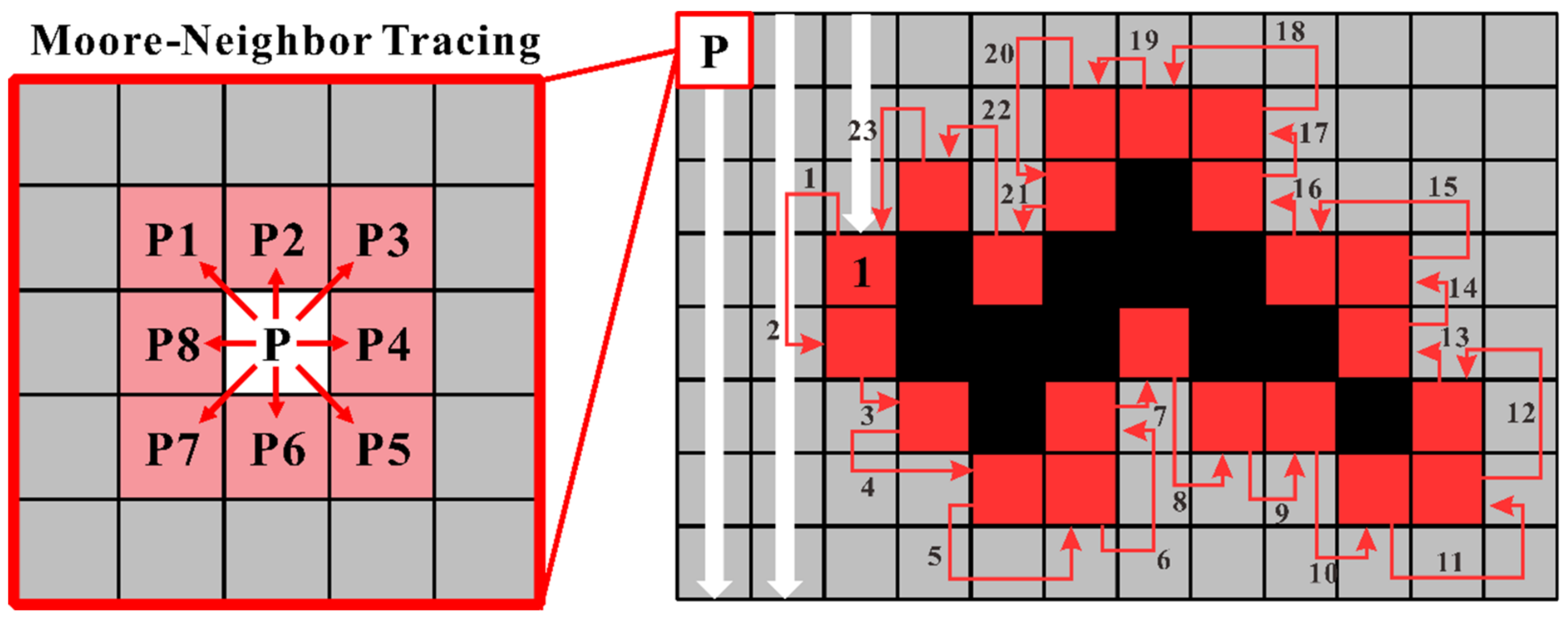
Finally, the performance of the boundary tracing algorithm is assessed. As shown in Figure 13, the proposed method successfully traced the grain boundary from a binary image. This algorithm can effectively distinguish between the grain, grain boundary, and background. The reconstruction ability of the tracing algorithm is related to the performance of the binarization process since the algorithm works based on the binary logic step to determine whether there is an absolute discontinuity in the binary value. Furthermore, the boundary coordinates of the specific grains were extracted from the results and integrated with the coordinate values obtained from image stitching and matching. From these steps, we recorded the location of the grain on the global coordinates (Figure 13c). This approach can be widely utilized for the observation of metal grains, such as the analysis of the geometry, grain area, and deformation.

5. Application for Tracking the Direction of Metal Grain Deformation

Once the proposed algorithms are integrated, the observer can extract the boundary of a specific grain target and trace its location on global coordinates. This allows for a further analysis to understand the metal grain deformation. One the application proposed in this study is integrated processing for tracking the direction of the grain deformation, which works based on the understanding that the area inside the GB on the equiaxed structure will expand owing to the plastic force [66]. In addition, the elastic force also will cause a transverse elongation and axial compression on the GB with respect to the Poisson ratio. Furthermore, the GB of the specific grain targets is extracted on the initial condition and after experiencing loads and then being stacked on the global coordinates. To track the shifting value of the grain deformation in detail, a basic unit in the finite-element analysis (FEA) was initiated to generate the quadratic mesh elements on the GB poly shapes with the same element size limits (Figure 14a,b). The shifting of the mesh element coordinates before and after the deformation was the input for calculating the direction of grain deformation. Unfortunately, the direct integration of the elements led to ambiguous results owing to the unbalanced number of nodes. Because of the deformed geometry, the GB area after the deformation was somewhat expanded, thus increasing the number of elements in the mesh. Thus, the corresponding nodes before and after the deformation were sequentially traced using the minimum variance value of the coordinate shift, which synchronized the mesh element on the GB area and matched the corresponding nodes. Finally, the deformation direction was arranged using a quiver plot on the Cartesian coordinates according to the shifting value of the optimized nodes (Figure 14c). To amplify the directional signals, the O-grid generalization method was applied to the results (Figure 14d). This technique was chosen because of the difference in the concentrations of the nodes near the GB and at the center of the grain. The O-grid technique works by calculating the average direction trend based on four corresponding grid areas near the starting point and amplifying the minority nodes to make them uniform.

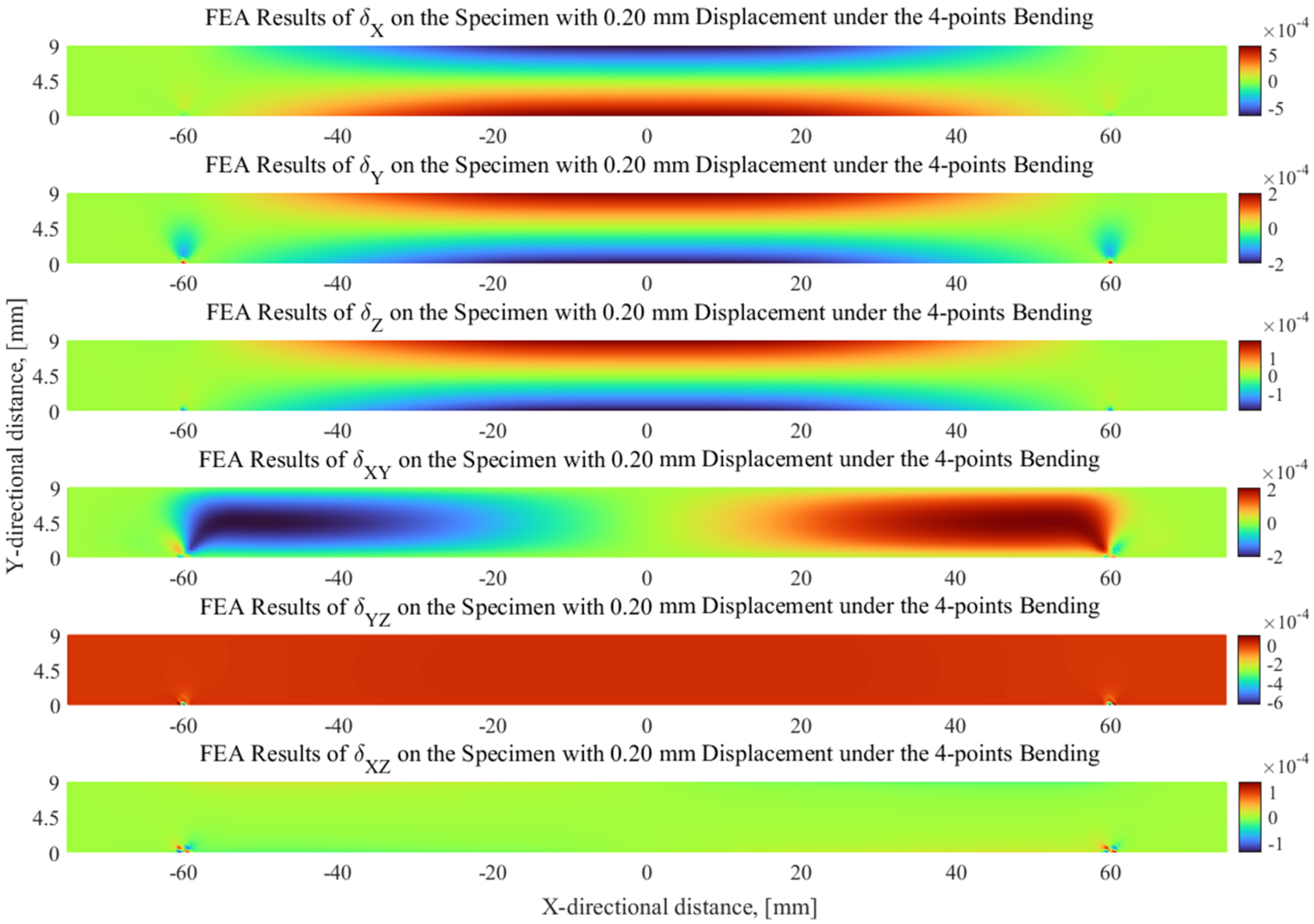
As an example of the implementation, FEA analysis was performed for a comparison, including deflection in the x (${\delta }_x$), y (${\delta }_y$), and z (${\delta }_z$) directions and the shear deflection in the xy (${\delta }_{XY}$), yz (${\delta }_{YZ}$), and xz (${\delta }_{XZ}$) directions (Figure 15). The strain vector at three specific locations, i.e., the compressive (A), combination (B), and tensile (C) stress areas, was assessed using a four-point bending test (Figure 16). After applying a deflection of 0.2 mm to the system according to the FEA analysis, uniform deformations of 0.511 μm, 0.013 nm, and 0.511 μm were expected to occur in regions A, B, and C, respectively. However, in the grain-level assessment using the proposed algorithm, the deformation did not occur in a uniform direction. As shown in Figure 16a, in the specific analysis in location A, where a compressive deformation of 0.511 μm was expected to occur owing to the compressive stress, there was an internal compression with the maximum magnitude of 0.433 μm. Likewise, at location B, where a deformation of 0.013 nm was expected owing to the compressive and tensile stresses, the compression and local shear stress of 0.154 μm was observed at the top and 0.077 μm at the bottom, as shown in Figure 16b. At location C, as shown in Figure 16c, where a deformation of approximately 0.511 μm was expected owing to the tensile stress, the local shear stress on the grain of 0.232 μm at the top and 0.310 μm at the bottom was clearly observed. It is related to the normal and shear stress on a boundary in a homogeneous body corresponding to the boundary orientation [67]. This result implies that the deformation analysis obtained by the numerical–analytical approach of the stress–strain on specific structures is very difficult to apply at the grain level (Figure 17). However, the experimental approach to the stress–strain in a specific region using a metallographic observation can effectively provide a high spatial resolution for tracing the microscopic deformation at the grain level. Thus, it is suggested that the algorithm proposed in this study is a tool to quantitatively measure the micro-deformation at the metal grain level (Figures S16–S18).

6. Conclusions

The main idea in this paper is to integrate a specific section view of the grain target with a view of the entire material surface for the tracking of the direction of the metal grain deformation. Several positive results were obtained in this study by successfully preventing performance drops during simultaneous training processes. GD-HBT successfully binarized gray-level metal grain images using a dynamic Gaussian threshold separator. When comparing with those of three existing binarization algorithms, it was shown that GD-HBT outperformed the existing algorithms. This intuitively explains why using the unique properties of each polycrystalline image as the threshold for image binarization reduced the structural degradation of the grain parts. Similarly, the proposed image-stitching algorithm based on BLM successfully reconstructed the view of the entire material surface. The connection of each image at the edge provided an appropriate overlap point as qualitative and quantitative evidence with homoscedasticity was performance on all datasets. The grain-matching algorithm testing using open-source FDs yielded positive results with a relatively low bias and variance. The results are also supported by the SE, t-statistic, and p-value values recorded during the testing, which were identical for each FD. Finally, the boundary extraction successfully traced the grain boundary from a binary image. This algorithm effectively distinguished between the grain, grain boundary, and background.

Despite the impressive toolset performance, the tracing, tracking, and reconstruction capabilities of the algorithms are not limitless. Ambiguous experimental results were found from the datasets with a significant ratio of the grain targets to the disturbance (the mounting area). Because the algorithm was designed based on binary matching to provide a fast feature detection, the mounting area was extracted without any unique features (blank spots), and thus this area did not provide a sufficient trigger for the algorithm to determine an anchor point. Additionally, considering that binarization is the most important process for achieving a high-precision grain boundary extraction, adjustments should always be made to improve GD-HBT as a binarization tool. The careless implementation of the thresholding values amplifies the possibility of a feature loss during the extraction.

Finally, the integrated algorithm was utilized as a tool to quantitatively measure micro-deformation at the metal grain level. This provided an effective method for calculating the direction of the grain deformation by comparing the overlapping area when the material experienced a load. The grain-level assessment using the proposed algorithm found that the microscopic deformation on the grain did not occur in a uniform direction. The are several magnitude deformation variations on the compressive stress area and a local shear stress appears inside the grain on the tensile and combination stress area. It is related to the normal and shear stress on a boundary in a homogeneous body corresponding to the boundary orientation, which is lacking in structural simulation, using FEA to achieve a grain-level assessment.

Ultimately, future research directions include improving image pre-processing to enhance the performance of the integrated toolsets, such as reducing the extraction error and feature loss while avoiding overfitting of the models. In addition, the improvement in matching the shifted quadratic mesh elements before and after the deformation to correlate the corresponding nodes can lead to a sophisticated stress–strain heatmap on the grain level, which is lacking in the literature. This improvement is expected to support further creative applications that require expeditious toolsets to observe fascinating phenomena in material science and engineering.

References

1. Knezevic, M.; Drach, B.; Ardeljan, M.; Beyerlein, I.J. Three Dimensional Predictions of Grain Scale Plasticity and Grain Boundaries Using Crystal Plasticity Finite Element Models. Comput. Methods Appl. Mech. Eng. 2014, 277, 239–259. [Google Scholar] [CrossRef]
2. Song, B.; Wen, S.; Yan, C.; Wei, Q.; Shi, Y. Materials characterization. In Selective Laser Melting for Metal and Metal Matrix Composites; Academic Press: Cambridge, MA, USA, 2021; pp. 231–247. [Google Scholar] [CrossRef]
3. Kumar, C.; Paul, C.P.; Das, M.; Bindra, K.S. Fiber Laser Welding of Ti-6Al-4V alloy. In Advanced Welding and Deforming; Elsevier: Amsterdam, The Netherlands, 2021; pp. 23–66. [Google Scholar] [CrossRef]
4. Di Gianfrancesco, A. Technologies for chemical analyses, microstructural and inspection investigations. In Materials for Ultra-Supercritical and Advanced Ultra-Supercritical Power Plants; Woodhead Publishing: Philadelphia, PA, USA, 2017; pp. 197–245. [Google Scholar] [CrossRef]
5. Radford, D.W. 3.13 Application of high temperature polymer matrix composites to engine intake valves. In Comprehensive Composite Materials II; Elsevier: Amsterdam, The Netherlands, 2018; pp. 312–349. [Google Scholar] [CrossRef]
6. El-Eskandarany, M.S. Mechanically induced solid-state amorphization. In Mechanical Alloying; William Andrew Publishing: Norwich, NY, USA, 2020; pp. 335–416. [Google Scholar] [CrossRef]
7. Dutta, B.; Babu, S.; Jared, B. Design for metal additive manufacturing. In Science, Technology and Applications of Metals in Additive Manufacturing; Elsevier: Amsterdam, The Netherlands, 2019; pp. 193–244. [Google Scholar] [CrossRef]
8. Sankaran, K.K.; Mishra, R.S. Titanium alloys. In Metallurgy and Design of Alloys with Hierarchical Microstructures; Elsevier: Amsterdam, The Netherlands, 2017; pp. 177–288. [Google Scholar] [CrossRef]
9. Mercier, J.P.; Zambelli, G.; Kurz, W. Microstructures. In Introduction to Materials Science; Elsevier: Amsterdam, The Netherlands, 2002; pp. 239–259. [Google Scholar] [CrossRef]
10. Dutta, B. Directed Energy Deposition (DED) technology. In Encyclopedia of Materials: Metals and Alloys; Elsevier: Amsterdam, The Netherlands, 2022; pp. 66–84. [Google Scholar] [CrossRef]
11. Panemangalore, D.B.; Shabadi, R. Microstructural aspects of metal-matrix composites. In Encyclopedia of Materials: Composites; Elsevier: Amsterdam, The Netherlands, 2021; pp. 274–297. [Google Scholar] [CrossRef]
12. Yuan, H.; Barbieri, D.; Luo, X.; van Blitterswijk, C.A.; de Bruijn, J.D. 1.14 Calcium phosphates and bone induction. In Comprehensive Biomaterials II; Elsevier: Amsterdam, The Netherlands, 2017; pp. 333–349. [Google Scholar] [CrossRef]
13. Chatterjee, S.; Mahapatra, S.S.; Behera, A. NiTi joining with other metallic materials. In Nickel-Titanium Smart Hybrid Materials: From Micro- to Nano-Structured Alloys for Emerging Applications; Elsevier: Amsterdam, The Netherlands, 2022; pp. 379–398. [Google Scholar] [CrossRef]
14. Chang, C.S.; He, J.L.; Lin, Z.P. The Grain Size Effect on the Empirically Determined Erosion Resistance of CVD-ZnS. Wear 2003, 255, 115–120. [Google Scholar] [CrossRef]
15. Opiela, M.; Fojt-Dymara, G.; Grajcar, A.; Borek, W. Effect of Grain Size on the Microstructure and Strain Hardening Behavior of Solution Heat-Treated Low-C High-Mn Steel. Materials 2020, 13, 1489. [Google Scholar] [CrossRef] [PubMed] [Green Version]
16. Wang, S.; Waggoner, J.; Simmons, J. Graph-Cut Methods for Grain Boundary Segmentation. JOM 2011, 63, 49–51. [Google Scholar] [CrossRef]
17. Sabzi, A.K.; Hasanzadeh, R.P.R.; Chegini, A.H.N. An Image-Based Object Tracking Technique for Identification of Moving Sediment Grains on Bed Deposits. KSCE J. Civ. Eng. 2018, 22, 1170–1178. [Google Scholar] [CrossRef]
18. Han, S.-M.; Lee, S.-M.; Kang, S.-J.L. Phase transformation and microstructure development in silicon nitride based materials. In Advanced Materials ’93; Elsevier: Amsterdam, The Netherlands, 1994; pp. 851–856. [Google Scholar] [CrossRef]
19. Fuchs Structure of Metals. Crystallographic Methods, Principles, and Data. Mater. Corros. 1954, 5, 37. [Google Scholar] [CrossRef]
20. Shan, Z.; Stach, E.A.; Wiezorek, J.M.K.; Knapp, J.A.; Follstaedt, D.M.; Mao, S.X. Grain Boundary-Mediated Plasticity in Nanocrystalline Nickel. Science 2004, 305, 654–657. [Google Scholar] [CrossRef]
21. Rupert, T.J.; Gianola, D.S.; Gan, Y.; Hemker, K.J. Experimental Observations of Stress-Driven Grain Boundary Migration. Science 2009, 326, 1686–1690. [Google Scholar] [CrossRef] [Green Version]
22. Gu, X.W.; Loynachan, C.N.; Wu, Z.; Zhang, Y.-W.; Srolovitz, D.J.; Greer, J.R. Size-Dependent Deformation of Nanocrystalline Pt Nanopillars. Nano Lett. 2012, 12, 6385–6392. [Google Scholar] [CrossRef]
23. Hu, J.; Shi, Y.N.; Sauvage, X.; Sha, G.; Lu, K. Grain Boundary Stability Governs Hardening and Softening in Extremely Fine Nanograined Metals. Science 2017, 355, 1292–1296. [Google Scholar] [CrossRef]
24. Wagdy, M.; Faye, I.; Rohaya, D. Document Image Binarization Using Retinex and Global Thresholding. ELCVIA Electron. Lett. Comput. Vis. Image Anal. 2015, 14, 61–73. [Google Scholar] [CrossRef]
25. Vikram Mutneja, D. Methods of Image Edge Detection: A Review. J. Electr. Electron. Syst. 2015, 4, 5. [Google Scholar] [CrossRef] [Green Version]
26. Mustafa, W.A.; Abdul Kader, M.M.M. Binarization of Document Images: A Comprehensive Review. J. Phys. Conf. Ser. 2018, 1019, 012023. [Google Scholar] [CrossRef] [Green Version]
27. Mlsna, P.A.; Rodríguez, J.J. Gradient and laplacian edge detection. In Handbook of Image and Video Processing; Elsevier: Amsterdam, The Netherlands, 2005; pp. 535–553. [Google Scholar]
28. Jing, J.; Liu, S.; Wang, G.; Zhang, W.; Sun, C. Recent Advances on Image Edge Detection: A Comprehensive Review. Neurocomputing 2022, 503, 259–271. [Google Scholar] [CrossRef]
29. Gonzalez, R.C.; Woods, R.E. Digital Image Processing, 3rd ed.; Prentice-Hall, Inc.: Hoboken, NJ, USA, 2006; ISBN 013168728X. [Google Scholar]
30. Sauvola, J.; Pietikäinen, M. Adaptive Document Image Binarization. Pattern Recognit. 2000, 33, 225–236. [Google Scholar] [CrossRef] [Green Version]
31. Davies, E.R. Binary shape analysis. In Computer Vision; Academic Press: Cambridge, MA, USA, 2018; pp. 203–238. [Google Scholar] [CrossRef]
32. Dharmawan, I.D.M.O.; Lee, J.; Sim, S. Defect Shape Classification Using Transfer Learning in Deep Convolutional Neural Network on Magneto-Optical Nondestructive Inspection. Appl. Sci. 2022, 12, 7613. [Google Scholar] [CrossRef]
33. Lee, J.; Berkache, A.; Wang, D.; Hwang, Y.-H. Three-Dimensional Imaging of Metallic Grain by Stacking the Microscopic Images. Appl. Sci. 2021, 11, 7787. [Google Scholar] [CrossRef]
34. Iwaszenko, S.; Smoliński, A. Texture Features for Bulk Rock Material Grain Boundary Segmentation. J. King Saud Univ. Eng. Sci. 2021, 33, 95–103. [Google Scholar] [CrossRef]
35. Panda, A.; Naskar, R.; Pal, S. Deep Learning Approach for Segmentation of Plain Carbon Steel Microstructure Images. IET Image Process. 2019, 13, 1516–1524. [Google Scholar] [CrossRef]
36. Haralick, R.M.; Sternberg, S.R.; Zhuang, X. Image Analysis Using Mathematical Morphology. IEEE Trans. Pattern Anal. Mach. Intell. 1987, PAMI-9, 532–550. [Google Scholar] [CrossRef]
37. Razavian, R.S.; Greenberg, S.; McPhee, J. Biomechanics Imaging and Analysis. In Encyclopedia of Biomedical Engineering; Elsevier: Amsterdam, The Netherlands, 2019; Volume 1–3, pp. 488–500. [Google Scholar] [CrossRef]
38. Lowe, D.G. Object Recognition from Local Scale-Invariant Features. In Proceedings of the Seventh IEEE International Conference on Computer Vision, Kerkyra, Greece, 20–27 September 1999; Volume 2, pp. 1150–1157. [Google Scholar]
39. Bay, H.; Ess, A.; Tuytelaars, T.; van Gool, L. Speeded-Up Robust Features (SURF). Comput. Vis. Image Underst. 2008, 110, 346–359. [Google Scholar] [CrossRef]
40. Rosten, E.; Drummond, T. Machine Learning for High-Speed Corner Detection. Comput. Vis. 2006, 3951, 430–443. [Google Scholar]
41. Calonder, M.; Lepetit, V.; Strecha, C.; Fua, P. BRIEF: Binary Robust Independent Elementary Features. In Proceedings of the 11th European Conference on Computer Vision, Heraklion, Greece, 5–11 September 2010; pp. 778–792. [Google Scholar]
42. Leutenegger, S.; Chli, M.; Siegwart, R.Y. BRISK: Binary Robust Invariant Scalable Keypoints. In Proceedings of the 2011 International Conference on Computer Vision, Barcelona, Spain, 6–13 November 2011; pp. 2548–2555. [Google Scholar]
43. Alahi, A.; Ortiz, R.; Vandergheynst, P. FREAK: Fast Retina Keypoint. In Proceedings of the 2012 IEEE Conference on Computer Vision and Pattern Recognition, Providence, RI, USA, 16–21 June 2012; pp. 510–517. [Google Scholar]
44. Wang, L.; Zhang, Y.; Zeng, Z.; Zhou, H.; He, J.; Liu, P.; Chen, M.; Han, J.; Srolovitz, D.J.; Teng, J.; et al. Tracking the Sliding of Grain Boundaries at the Atomic Scale. Science 2022, 375, 1261–1265. [Google Scholar] [CrossRef] [PubMed]
45. Dufaux, F. Grand Challenges in Image Processing. Front. Signal Process. 2021, 1, 675547. [Google Scholar] [CrossRef]
46. Chen, L.; Rottensteiner, F.; Heipke, C. Feature Detection and Description for Image Matching: From Hand-Crafted Design to Deep Learning. Geo-Spat. Inf. Sci. 2021, 24, 58–74. [Google Scholar] [CrossRef]
47. Ueda, J.; Schultz, J.A.; Asada, H.H. Application of cellular actuators. In Cellular Actuators; Butterworth-Heinemann: Oxford, UK, 2017; pp. 213–276. [Google Scholar] [CrossRef]
48. ASTM International. ASTM E3-11: Standard Guide for Preparation of Metallographic Specimens; McCall, J.L., Mueller, W.M., Eds.; Springer: Boston, MA, USA, 2012. [Google Scholar]
49. Yadav, G.; Maheshwari, S.; Agarwal, A. Contrast Limited Adaptive Histogram Equalization Based Enhancement for Real Time Video System. In Proceedings of the 2014 International Conference on Advances in Computing, Communications and Informatics (ICACCI), Delhi, India, 24–27 September 2014; pp. 2392–2397. [Google Scholar]
50. Kuran, U.; Kuran, E.C. Parameter Selection for CLAHE Using Multi-Objective Cuckoo Search Algorithm for Image Contrast Enhancement. Intell. Syst. Appl. 2021, 12, 200051. [Google Scholar] [CrossRef]
51. Lewis, J.P. Fast Normalized Cross-Correlation. Vis. Interfaces 1995, 120–123. [Google Scholar]
52. Haralick, R.M.; Shapiro, L.G. Computer and Robot Vision, 1st ed.; Addison-Wesley Longman Publishing Co., Inc.: Boston, MA, USA, 1992; ISBN 0201569434. [Google Scholar]
53. Cui, Z.; Qi, W.; Liu, Y. A Fast Image Template Matching Algorithm Based on Normalized Cross Correlation. J. Phys. Conf. Ser. 2020, 1693, 012163. [Google Scholar] [CrossRef]
54. Briechle, K.; Hanebeck, U.D. Template matching using fast normalized cross correlation. In Proceedings of the Aerospace/Defense Sensing, Simulation, and Controls Conference, Orlando, FL, USA, 16–20 April 2001; pp. 95–102. [Google Scholar] [CrossRef]
55. Tsai, D.-M.; Lin, C.-T. Fast Normalized Cross Correlation for Defect Detection. Pattern Recognit. Lett. 2003, 24, 2625–2631. [Google Scholar] [CrossRef]
56. Yoo, J.-C.; Han, T.H. Fast Normalized Cross-Correlation. Circuits Syst. Signal Process. 2009, 28, 819–843. [Google Scholar] [CrossRef]
57. Reddy, P.R.; Amarnadh, V.; Bhaskar, M. Evaluation of Stopping Criterion in Contour Tracing Algorithms. (IJCSIT) Int. J. Comput. Sci. Inf. Technol. 2012, 3, 3888–3894. [Google Scholar]
58. Bayar, G. Increasing Measurement Accuracy of a Chickpea Pile Weight Estimation Tool Using Moore-Neighbor Tracing Algorithm in Sphericity Calculation. J. Food Meas. Charact. 2021, 15, 296–308. [Google Scholar] [CrossRef]
59. Sharma, P.; Diwakar, M.; Lal, N. Edge Detection Using Moore Neighborhood. Int. J. Comput. Appl. 2013, 61, 26–30. [Google Scholar] [CrossRef]
60. Otsu, N. A Threshold Selection Method from Gray-Level Histograms. IEEE Trans. Syst. Man. Cybern. 1979, 9, 62–66. [Google Scholar] [CrossRef] [Green Version]
61. Bradley, D.; Roth, G. Adaptive Thresholding Using the Integral Image. J. Graph. Tools 2007, 12, 13–21. [Google Scholar] [CrossRef]
62. Harris, C.; Stephens, M. A Combined Corner and Edge Detector. In Proceedings of the 4th Alvey Vision Conference, Manchester, UK, 31 August–2 September 1988; pp. 23.1–23.6. [Google Scholar]
63. Obdržálek, D.; Basovník, S.; Mach, L.; Mikulík, A. Detecting Scene Elements Using Maximally Stable Colour Regions. In Proceedings of the Research and Education in Robotics—EUROBOT 2009 International Conference, La Ferté-Bernard, France, 21–23 May 2009; Springer: Berlin/Heidelberg, Germany, 2010; pp. 107–115. [Google Scholar]
64. Rublee, E.; Rabaud, V.; Konolige, K.; Bradski, G. ORB: An Efficient Alternative to SIFT or SURF. In Proceedings of the 2011 International Conference on Computer Vision, Barcelona, Spain, 6–13 November 2011; pp. 2564–2571. [Google Scholar]
65. Bay, H.; Tuytelaars, T.; van Gool, L. SURF: Speeded Up Robust Features. In Proceedings of the 9th European Conference on Computer Vision, Graz, Austria, 7–13 May 2006; pp. 404–417. [Google Scholar]
66. Bate, P.S.; Hutchinson, W.B. Grain Boundary Area and Deformation. Scr. Mater 2005, 52, 199–203. [Google Scholar] [CrossRef]
67. Beere, W.; Rutter, E.H. Stresses and Deformation at Grain Boundaries [and Discussion]. Philos. Trans. R. Soc. London. Ser. A Math. Phys. Sci. 1978, 288, 177–196. [Google Scholar]
68. JCGM 100:2008; Evaluation of Measurement Data-Guide to the Expression of Uncertainty in Measurement. ISO: Geneva, Switzerland, 2008.
Figure 1. Comparison of edge detection algorithm using gradient and Laplacian filter: (a) gray-level and (b) binary images.
Applsci 13 00045 g001
Figure 2. Experimental setup for data acquisition process and geometric analysis of grain boundary using integrated image processing toolsets: (a) optical microscopy setup, (b) mounted specimen, and (c) X-Y-Z stage motor controller based on LabVIEW, (d) microscope user interface, (e) experimental flow chart.
Applsci 13 00045 g002
Figure 3. Experimental setup of 4-point bending test: (a) geometric view and (b) top view. The observation was conducted in compressive, tensile, and a combination of compressive and tensile stress areas.
Applsci 13 00045 g003
Figure 4. Flow chart of microscope image-stitching algorithm: image binarization using Gaussian dynamic histogram brightness transformation (GD-HBT), image binary logic matching, and data stacking.
Applsci 13 00045 g004
Figure 5. Heatmap analysis of BLM algorithm and its visualization for computing pixel similarity.
Applsci 13 00045 g005
Figure 6. Fast normalized cross-correlation (f-NCC) algorithm for grain matching: (a) reference image: stitched 50-scope, (b) target image: 200-scope, (c) normalized cross-correlation analysis, (d) plot of target image location on the reference image, (e) surface plot of correlation map, and (f) stacking analysis of 200-scope image (bright) on stitched 50-scope image (dark).
Applsci 13 00045 g006
Figure 7. Visualization of implementation of Moore–Neighbor tracing algorithm with modification of the tracing termination using Jacob’s stopping criteria for grain boundary extraction.
Applsci 13 00045 g007
Figure 8. Confusion matrix analysis of GD-HBT algorithm on image binarization performance.
Applsci 13 00045 g008
Figure 9. The final results of the 50-scope stitched image and analysis of training time: (a) raw and (b) weld specimens.
Applsci 13 00045 g009
Figure 10. Heatmap analysis of confidence value on 50-scope datasets: (a) raw and (b) weld specimens.
Applsci 13 00045 g010
Figure 11. Linear regression model analysis based on least-squares methods for assessing the model performance and behavior.
Applsci 13 00045 g011
Figure 12. Linear regression model analysis based on least-squares methods for assessing the model performance and behavior.
Applsci 13 00045 g012
Figure 13. Grain boundary extraction processes: (a) target grain labelling using built-it MATLAB apps “Image Labeler”, (b) extraction results using Moore–Neighbor tracing algorithm with updated Jacob’s stopping criteria, (c) plot of specific grain on global location coordinate by integrating the stitched image, matching, and boundary coordinate.
Applsci 13 00045 g013
Figure 14. Implementation of the integrated toolsets for extracting the direction of grain deformation: (a) geometric meshing analysis on grain before deformation, (b) geometric meshing analysis on grain after deformation, (c) quiver plot of direction of metal grain deformation, and (d) O-grid generalization method to amplify the trend of direction signal.
Applsci 13 00045 g014
Figure 15. The results of numerical approach using FEA on structural simulation of 4-point bending test including deflection components in the x ( δ x , y ( δ x ), and z ( δ x ) directions and shear deflection in the xy ( δ X Y ), yz ( δ Y Z ), and xz ( δ X Z ) directions.
Applsci 13 00045 g015
Figure 16. The grain-level analysis of deformation direction for understanding the internal deformation trends on the grain area: (a) compressive stress area, (b) compressive and tensile stress area, and (c) tensile stress area.
Applsci 13 00045 g016
Figure 17. Vector plot of FEA of deflection components in the x ( δ x ) vs. y ( δ y ), on structural simulation of 4-point bending test.
Applsci 13 00045 g017