Article

Research on Yaw Stability Control Method of Liquid Tank Semi-Trailer on Low-Adhesion Road under Turning Condition

School of Mechanical and Electronical Engineering, Wuhan University of Technology, Wuhan 430070, China
*
Author to whom correspondence should be addressed.
Appl. Sci. 2023, 13(1), 39; https://doi.org/10.3390/app13010039
Submission received: 25 November 2022 / Revised: 16 December 2022 / Accepted: 16 December 2022 / Published: 21 December 2022

Abstract

:
To ensure that a liquid tank semi-trailer has good yaw stability and path-following performance on low-adhesion roads under turning conditions, a multi-object PID differential braking-control method is proposed, which takes the tractor yaw rate, semi-trailer yaw rate, and articulation angle as the control parameters. According to the principle of equivalence, the trammel pendulum (TP) model is used to simulate the liquid sloshing effect in the liquid tank, and the Fluent software is used to identify the key parameters of the trammel pendulum model and verify the correctness of its simulation effect. Then, a co-simulation model is built based on TruckSim and MATLAB/Simulink. Based on the simplified six degrees of freedom model and the co-simulation model of a liquid tank semi-trailer, a multi-object PID differential braking-control method is designed, and the vehicle state responses with and without control are compared when it is turning on a low-adhesion road. The simulation results show that the proposed multi-object PID differential braking-control method can effectively improve the yaw stability and path-following performance of the liquid tank semi-trailer when turning on a low-adhesion road.

1. Introduction

With its large transportation capacity and low transportation cost, the liquid tank semi-trailer has become the main vehicle for transporting liquid chemical products. Compared with ordinary freight cars, liquid tank semi-trailers not only have the characteristics of a high center of mass position and large cargo weight but also are more prone to instability than ordinary semi-trailers, because of the coupling relationship between the lateral sloshing of the liquid in the tank and the tank body [1].
The dangerous working conditions of liquid tank semi-trailers are mainly divided into yaw instability and roll instability. When a vehicle is running on a low-adhesion road, due to the small adhesion between the tires and the road, the lateral force of the tires is easy to become saturated, which leads to the occurrence of yaw instability; when driving on a high adhesion road, a vehicle is prone to roll instability [2]. At present, most scholars’ research mainly focuses on the influencing factors and improved methods of the roll stability of liquid tank semi-trailers. Li, X. [3] established a dynamic model of a liquid tank vehicle based on the trammel pendulum (TP) model and analyzed the influence of the liquid filling ratio and other influencing factors on the driving stability of the liquid tank vehicle. Peng, G. [4] established a volume of fluid (VOF) multi-phase flow model and a standard k-ε turbulence model to study the effects of transportation conditions, such as the liquid-filling ratio, the elliptical ratio of the tank section, and the number of baffles, on the vehicle’s roll stability. Saeedi, M.A. [5] improved the roll stability of a liquid-carrying articulated vehicle based on the proposed two control methods to avoid rollover, shimmy, and folding accidents.
These studies analyzed the influencing factors of the roll stability of a liquid tank semi-trailer on a good road and provided the corresponding improvement methods, but there were few studies on the yaw stability of vehicles turning on low-adhesion roads. In addition, most research on the path-following problem concentrates on the field of intelligent vehicles [6], while little research focuses on the field of heavy semi-trailers or liquid tank semi-trailers. Therefore, this paper studies the yaw stability and path-following performance of liquid tank semi-trailers when turning on low-adhesion roads.
To study the yaw stability control method of liquid tank semi-trailers when driving on low-adhesion roads under turning conditions, it is necessary to study the liquid sloshing law in the tank. At present, the main research methods of liquid sloshing are hydrodynamics, the quasi-static model, the equivalent mechanical model, etc. [7]. With the ability to describe the large amplitude of liquid sloshing and the convenience of being coupled with the vehicle dynamic model, the equivalent mechanical model is widely used in practical engineering.
The most commonly used equivalent mechanical models mainly include the spring-mass model, the simple pendulum model, and the TP model [8]. However, the spring-mass model is only suitable for small amplitude shaking; for the simple pendulum model, the motion track of it is a circular arc, which is only suitable for describing the liquid sloshing effect in a cylindrical tank but not for an elliptical cylinder tank. To solve this problem, Salem [9] studied the liquid impact in the horizontal elliptical cylinder tank and proposed the TP model, which is suitable for simulating the liquid sloshing effect in the elliptical cylinder tank.
In terms of vehicle yaw stability control methods, there are mainly active steering, active suspension, differential braking, etc. [10]. Among these methods, the actuator of active steering is complex and costly, the damping adjustment range of active suspension is small, and the suspension adjustment time is too long. Differential braking generates the additional yaw moment by controlling the braking force of different wheels; since the hardware cost is low, it has been widely used [11].
In terms of control algorithms, the main methods include fuzzy PID control, optimal control, MPC control, sliding mode control, and other control algorithms [12]. Easy to use and not requiring a specific mathematical model to be obtained, the fuzzy PID control method is suitable for such highly nonlinear models as liquid tank semi-trailers.
In Section 2, according to the principle of equivalence, the TP model is taken to simulate the liquid sloshing effect in the liquid tank, and the Fluent software is used to verify the effectiveness. In Section 3, a simplified six degrees of freedom model of a liquid tank semi-trailer is built and verified based on TruckSim and MATLAB/Simulink; the control parameters and expected values are selected and determined. In Section 4, a multi-object PID differential braking-control method is designed; the calculation and distribution of the additional yaw moment are determined; and the wheel-slip-rate control method is introduced. In Section 5, the double-lane change and the step-steering-angle input working conditions are chosen to verify the effectiveness of the proposed method in improving the yaw stability and path-following performance of the liquid tank semi-trailer when running on a low-adhesion road; the robustness of the proposed method is also discussed and verified when the input disturbance pulses are included and the control parameters are changed.

2. Equivalent Model of Liquid Sloshing for the Liquid Tank Semi-Trailer and the Establishment of Its Co-Simulation Analysis Model

2.1. Equivalent Model of Liquid Sloshing for the Liquid Tank Semi-Trailer

The schematic diagram of the TP model is shown in Figure 1, and its symbols are explained in Table 1.
For the TP model, the liquid in the tank is divided into the sloshing part and the static part. The movement of the sloshing part is equivalent to the swing of the pendulum ball. The motion track is circular or elliptical and is similar to the tank section profile, which meets the following requirements:
l a l b = l a c g l b c g = l a p l b p = ζ
Based on Lagrange mechanics, the motion equation of the pendulum ball in the accelerated translational tank can be derived as follows [13]:
γ ¨ ( l a p 2 sin 2 γ + l b p 2 cos 2 γ ) + 1 2 γ ˙ 2 ( l a p 2 l b p 2 ) ( sin 2 γ g l b p cos γ a y l a p sin γ ) = 0
The lateral sloshing force F W on the tank caused by liquid sloshing is
F w = m p ( a y l a p γ ¨ sin γ l a p γ ˙ 2 cos γ ) + m s a y
The sloshing torque M w around the lowest point of the tank caused by liquid sloshing is
M w = m s a y l b s + m p | l a p cos γ l b l b p sin γ a y l a p ( γ ¨ sin γ + γ ˙ 2 cos γ ) l b p ( γ ˙ 2 sin γ γ ¨ cos γ ) + g |
The TP model parameters shall be determined using the parameter identification method. According to the equivalence principle of dynamic similarity, kinematic similarity, and geometric similarity [14], the simulation results of an elliptical cylinder tank under step excitation of unit lateral acceleration are simulated by fluid numerical simulation using the Fluent software for parameter identification, and the TP model parameters are obtained as shown in Table 1.

2.2. Verification of Equivalent Model of Liquid Sloshing for the Liquid Tank Semi-Trailer

To verify the accuracy of the TP model in simulating the liquid sloshing effect of the tank when subjected to lateral excitation, a typical liquid tank is selected, and its basic parameters are shown in Table 1. The time-varying lateral acceleration a y applied on the tank body is
a y = 0.2 g sin ( 0.4 t )
The Fluent software and the TP model are, respectively, used to simulate the sloshing force and torque generated by the liquid sloshing in the tank. The results are shown in Figure 2a,b.
It can be seen from Figure 2a,b that the magnitude and frequency of liquid sloshing force and torque obtained by the Fluent software and the TP model maintain good consistency, indicating that the TP model can simulate the liquid sloshing effect when the liquid in the tank is subjected to time-varying lateral excitation.

2.3. Co-Simulation Analysis Model of Liquid Sloshing Characteristics for the Liquid Tank Semi-Trailer

Considering the danger of the real vehicle test, a co-simulation model of the liquid tank semi-trailer is established based on TruckSim and MATLAB/Simulink, as shown in Figure 3. In this model, the lateral acceleration of the TruckSim model is input into the liquid sloshing model, and the liquid sloshing model outputs the force and torque generated by liquid sloshing to the TruckSim model [15].
As a famous simulation analysis software for commercial vehicles, TruckSim provides a data communication interface with MATLAB/Simulink. When the simulation test is carried out under different working conditions, it is only necessary to set the relevant structural parameters and driving conditions of the vehicle in TruckSim, set the input parameters and output parameters, and then generate the corresponding S function for Simulink to call to achieve the data communication between the two.
The TruckSim input/output setting module is shown in Figure 4, in which the input setting module’s Import Channel is the force and torque generated by liquid shaking, and the output setting module’s Output Channel is the lateral acceleration of the liquid tank semi-trailer.
For the TP model, it is written in the MATLAB function module in Simulink, which uses the ode45 function to solve the simulation test in real time, so the calculation step size should be consistent with that of TruckSim.

3. Simplified Six Degrees of Freedom Model and Control Parameters of the Liquid Tank Semi-Trailer for Yaw Stability Control

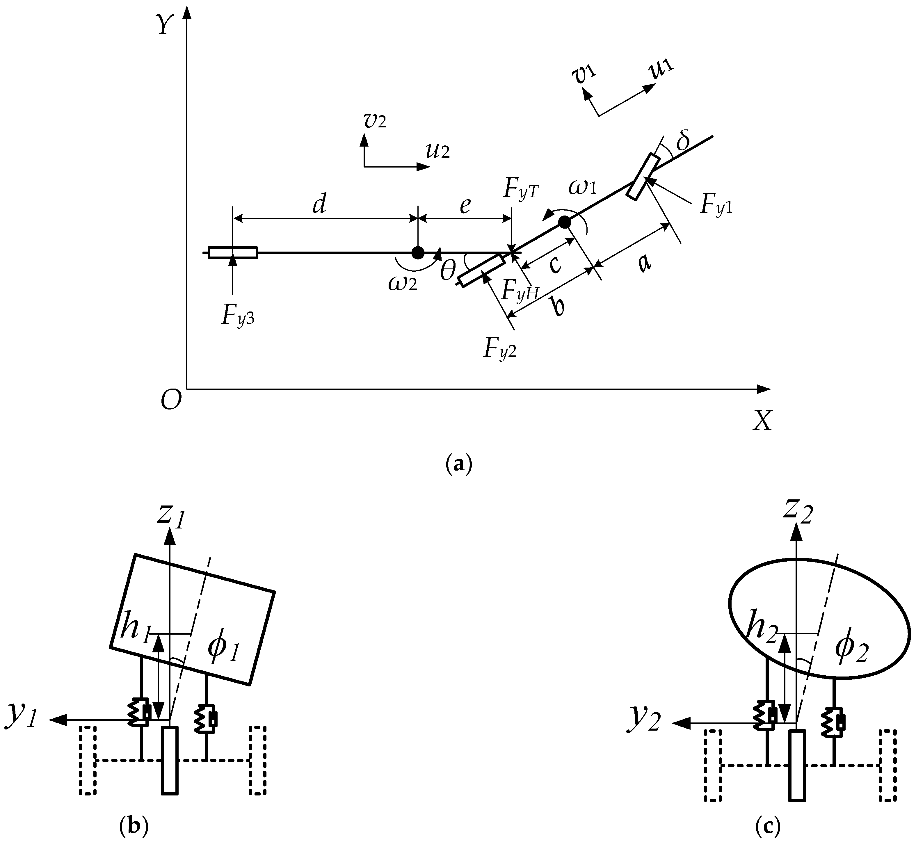
3.1. Simplified Six Degrees of Freedom Model of the Liquid Tank Semi-Trailer for Yaw Stability Control

In this paper, a six-axle liquid tank semi-trailer is selected for research. The schematic diagram of the single-track model of the vehicle is shown in Figure 5. Figure 5a shows the XOY plane layout of the selected vehicle, Figure 5b,c explain the roll motion between the sprung mass and the chassis when the vehicle is turning on a road. The origin point of the tractor and semi-trailer are, respectively, the intersection of the centroid cross section and its roll axis. The X-axis points to the front of the vehicle, the Y-axis points to the left of the driver, and the Z-axis points to the top of the vehicle.
According to the definition in Figure 5, considering the lateral, yaw, and roll motions of the tractor and semi-trailer, the differential motion equations of the two are listed as follows.
For the lateral motion of the tractor:
m 1 u 1 ( β ˙ 1 + ψ ˙ 1 ) m 1 s h 1 ϕ ¨ 1 = F y 1 cos δ + F y 2 + F y H
where m 1 is the mass of the tractor, kg ; m 1 s is the sprung mass of the tractor, kg ; u 1 is the longitudinal velocity of the tractor, m / s ; β 1 is the sideslip angle of the tractor’s center of mass, rad ; ψ ˙ 1 is the yaw rate of the tractor, rad / s ; ϕ ¨ 1 is the tractor roll angular acceleration, rad / s 2 ; F y i is the lateral force of wheel i ( i = 1 ,   2 ,   3 ) , N; F y H is the lateral force at the articulated point, N ; δ is the steering wheel angle, rad ; and h 1 is the distance from the tractor centroid to its roll axis, m .
For the yaw motion of the tractor:
I 1 z z ψ ¨ 1 I 1 x z ϕ ¨ 1 = F y 1 a cos δ F y 2 F y H c
where I 1 z z is the moment of inertia of the tractor around the Z axis, kg · m 2 ; I 1 x z is the centroid yaw-roll inertia product of the tractor, kg · m 2 ; a is the distance from the front axle of the tractor to its centroid, m ; and c is the distance from the tractor centroid to the articulated point, m .
For the roll motion of the tractor:
( I 1 x x + m 1 s h 1 2 ) ϕ ¨ 1 I 1 x z ψ ¨ 1 = m 1 s g h 1 sin ϕ 1 m 1 s + u 1 ( ( β ˙ 1 + ψ ˙ 1 ) h 1 ϕ ¨ 1 ) h 1 k r 1 ϕ 1 c 1 ϕ ˙ 1 + k 12 ( ϕ 2 ϕ 1 ) F y H h 1 c
where I 1 x x is the moment of inertia of the tractor around the X-axis, kg · m 2 ; h 1 c is the distance from the articulation point to the tractor roll axis, m; k r 1 is the roll stiffness of the tractor, N · m / rad ; c 1 is the roll damping of the tractor, N · m · s / rad ; k 12 is the coupling roll stiffness of the fifth wheel, N · m / rad .
For the lateral motion of the semi-trailer:
m 2 u 2 ( β ˙ 2 + ψ ˙ 2 ) m 2 s h 2 ϕ ¨ 2 = F y T + F y 3
where: m 2 is the mass of the semi-trailer, kg ; m 2 s is the sprung mass of the semi-trailer, kg ; u 2 is the longitudinal velocity of the semi-trailer, m / s ; β 2 is the sideslip angle of the semi-trailer, rad ; ψ ˙ 2 is the yaw rate of the semi-trailer, rad / s ; ϕ ¨ 2 is the roll angular acceleration of semi-trailer, rad / s 2 ; F y T is the lateral force at the articulated point, N; and h 2 is the distance from the centroid of the semi-trailer to its roll axis, m.
For the yaw motion of the semi-trailer:
I 2 z z ψ ¨ 2 I 2 x z ϕ ¨ 2 = F y T e F y 3 d
where I 2 z z is the moment of inertia of the semi-trailer around the Z axis, kg · m 2 ; I 2 x z is the centroid yaw-roll inertia product of the semi-trailer, kg · m 2 ; d is the distance from the axle of the semi-trailer to its center of mass, m; and e is the distance from the centroid of the semi-trailer to the articulated point, m.
For the semi-trailer roll movement:
( I 2 xx + m 2 s h 2 2 ) ϕ ¨ 2 I 2 x z ψ ¨ 2 = m 2 s g h 2 sin ϕ 2 + m 2 s ( u 2 ( β ˙ 2 + ψ ˙ 2 ) h 2 ϕ ¨ 2 ) h 2 + F y T h 2 c c 2 ϕ ˙ 2 k r 2 ϕ 2 k 12 ( ϕ 2 ϕ 1 )
where I 2 x x is the moment of inertia of the semi-trailer around the X-axis, kg · m 2 ; h 2 c is the distance from the articulated point to the roll axis of the semi-trailer, m ; k r 2 is the semi-trailer roll stiffness, N · m / rad ; and c 2 is semi-trailer roll damping, N · m · s / rad .
The constraint equation at the fifth wheel is as follows:
{ F y T = F y H cos θ θ ˙ = ψ ˙ 2 ψ ˙ 1 β 2 = β 1 h 1 c u 1 ϕ ˙ 1 + h 2 c u 2 ϕ ˙ 2 c u 1 ψ ˙ 1 e u 2 ψ ˙ 2 θ
The linear tire model is adopted for vehicle tires as follows:
{ F y 1 = k 1 α 1 = k 1 ( β 1 + a ψ ˙ 1 u δ ) F y 2 = k 2 α 2 = k 2 ( β 1 b ψ ˙ 1 u ) F y 3 = k 3 α 3 = k 3 ( β 2 d ψ ˙ 2 u )
where θ is the articulated angle, rad ; k i is the lateral stiffness of wheel i ( i = 1 ,   2 ,   3 ) , N / rad ; and α i is the side slip angle of wheel i, rad .
Combining Equations (6)–(13) and eliminating the fifth wheel force F y H , a simplified dynamic model of the liquid tank semi-trailer is obtained as follows:
M X ˙ = N X + K U
where X is the state variable, and X = [ β 1   ψ ˙ 1   ϕ 1   ϕ ˙ 1   ϕ 2   ϕ ˙ 2   θ ˙   θ ] T ; U is the input, and U = δ ;
Matrix M =
( c m 1 u 1 I 1 zz 0 I 1 xz c h 1 m 1 s 0 0 0 0 ( h 1 c m 1 h 1 m 1 s ) u 1 I 1 xz 0 m 1 s ( 2 h 1 2 h 1 c h 1 ) + I 1 xx 0 0 0 0 m 1 u 1 + m 2 u 2 e m 2 c m 2 u 2 u 1 0 h 1 m 1 s h 1 c m 2 u 2 u 1 0 h 2 c m 2 h 2 m 2 s e m 2 0 e m 2 u 2 I 2 zz + e 2 m 2 + c e m 2 u 2 u 1 0 e h 1 c m 2 u 2 u 1 0 e ( h 2 m 2 s h 2 c m 2 ) I 2 xz m 2 e 2 + I 2 zz 0 ( h 2 c m 2 h 2 m 2 s ) u 2 e ( h 2 m 2 s h 2 c m 2 ) I 2 xz + c ( h 2 m 2 s h 2 c m 2 ) u 2 u 1 0 h 1 c ( h 2 m 2 s h 2 c m 2 ) u 2 u 1 0 2 m 2 s ( h 2 h 2 c ) + m 2 h 2 c 2 + I 2 xx e ( h 2 m 2 s h 2 c m 2 ) I 2 xz 0 0 0 1 0 0 0 0 0 0 0 0 0 1 0 0 0 0 0 0 0 0 0 0 1 )
Matrix N =
( ( a + c ) k 1 ( b c ) k 2 ( a 2 + a c ) k 1 + ( b 2 b c ) k 2 u 1 c m 1 u 1 0 0 0 0 0 0 h 1 c ( k 1 + k 2 ) ( h 1 m 1 s h 1 c m 1 ) u 1 + ( a k 1 b k 2 ) h 1 c u 1 g h 1 m 1 s k r 1 k 12 c r 1 k 12 0 0 0 k 1 + k 2 + k 3 a k 1 b k 2 c k 3 u 1 m 2 u 2 m 1 u 1 ( d + e ) k 3 u 2 0 h 1 c k 3 u 1 0 h 2 c k 3 u 2 ( d + e ) k 3 u 2 k 3 d k 3 e k 3 ( d + e ) 2 k 3 u 2 + e m 2 u 2 + c ( d + e ) k 3 u 1 0 ( d + e ) h 1 c k 3 u 1 0 ( d + e ) h 2 c k 3 u 2 ( d + e ) 2 k 3 u 2 ( d + e ) k 3 h 2 c k 3 ( h 2 m 2 s h 2 c m 2 ) u 2 c h 2 c k 3 u 1 ( d + e ) h 2 c k 3 u 2 k 12 h 1 c h 2 c k 3 u 1 g h 2 m 2 s k r 2 k 12 h 2 c 2 k 3 u 2 c r 2 ( d + e ) h 2 c k 3 u 2 h 2 c k 3 0 0 0 1 0 0 0 0 0 0 0 0 0 1 0 0 0 0 0 0 0 0 1 0 )
Matrix K = [ ( a + c ) k 1 h 1 c k 1 k 1   0   0   0 ] T .

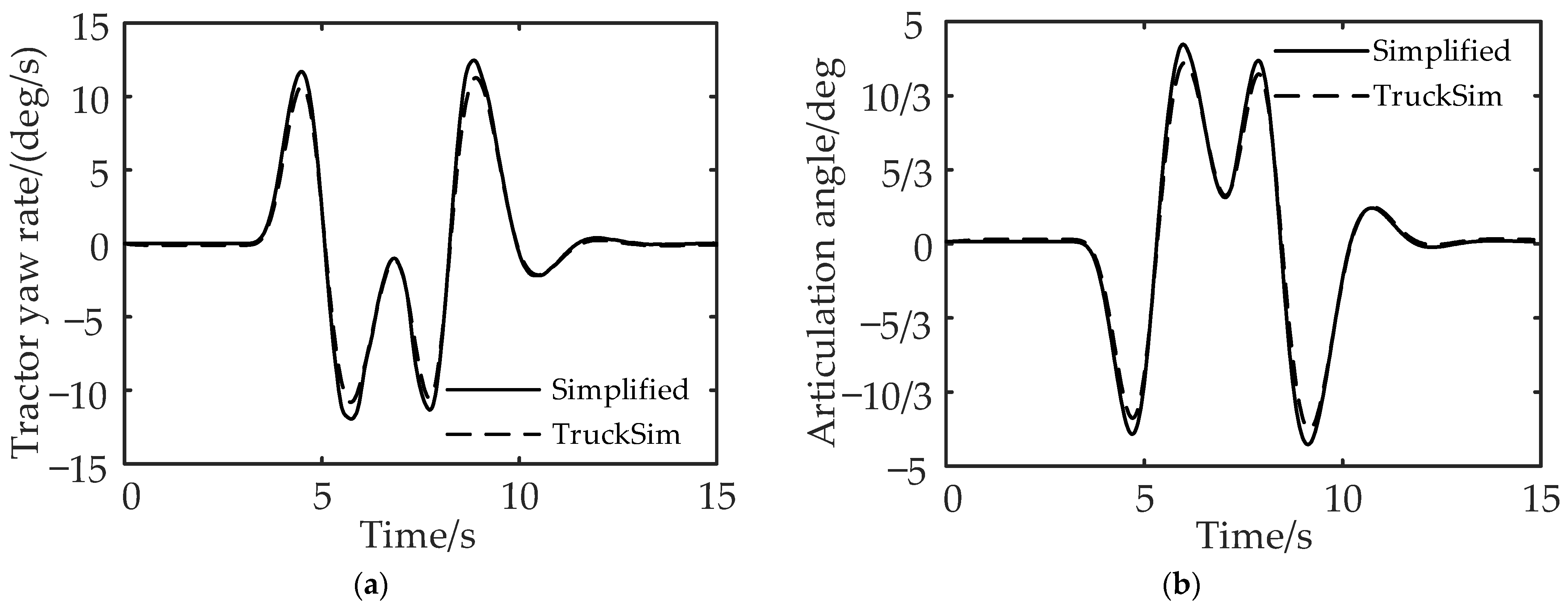
3.2. Verification of Simplified Six Degrees of Freedom Model of the Liquid Tank Semi-Trailer for Yaw Stability Control

To verify the accuracy of the simplified model for the liquid tank semi-trailer, the state responses of the simplified model and the TruckSim vehicle model under the double-lane shifting condition are compared. The initial vehicle speed is set to 80 km/h, the ground adhesion coefficient is 0.4, and the basic vehicle parameters are shown in Table 2.
It can be seen from Figure 6a,b that the established simplified six degrees of freedom model of the liquid tank semi-trailer can reflect the vehicle state and can be used for the development of the yaw stability control method of the liquid tank semitrailer.

3.3. Selection of Control Parameters for Yaw Stability Control of the Liquid Tank Semi-Trailer

In terms of the selection of the control parameters, the yaw rate, the sideslip angle of the centroid, and the lateral acceleration are generally taken for stability control [16]. When these variables are used for the control, the vehicle’s yaw stability will be greatly improved, but the driving path deviation would be produced compared with the path under steady-state driving. The magnitude of the articulated angle of the liquid tank semi-trailer directly reflects the steering characteristics and driving path of the liquid tank semi-trailer. The deviation of the driving path indicates the path-following ability of the semi-trailer to the tractor [17]. The greater the deviation is, the worse the path-following performance would be. Therefore, if the articulation angle can be adjusted to that of the steady state, while maintaining the stability of the vehicle’s yaw rate, the vehicle would have both good yaw stability and good path-following performance.
Therefore, the tractor yaw rate, the semi-trailer yaw rate, and the articulation angle are selected as the control parameters.

3.4. Determination of Expected Values for Yaw Stability Control Parameters of the Liquid Tank Semi-Trailer

When implementing the control method, it is necessary to obtain the vehicle state value when the vehicle is running stably, that is, the expected value of the vehicle state response. Take the derivative value of each state variable in the six degrees of freedom model of the liquid tank semi-trailer in Section 2.1 as zero, to obtain the vehicle linear reference model required by the control system, that is β 1 ˙ = ψ ¨ 1 = ϕ ˙ 1 = ϕ ¨ 1 = ϕ ˙ 2 = ϕ ¨ 2 = θ ˙ = 0 . Then, the expected value of each state variable under a stable state can be determined as X d :
{ X d = [ β 1 d   ψ ˙ 1 d   ϕ 1 d   ϕ 2 d   θ d ] T 0 = N d X d + K d U d
where U d is the system input, U d = δ ; K d is a 5 × 1 dimensional matrix, K d = [ ( a + c ) k 1 h 1 c k 1 k 1   0   0   0 ] T ; and N d is a 5 × 5 dimensional matrix.
N d = [ ( a + c ) k 1 + ( c b ) k 2 N d 12 0 0 0 ( k 1 + k 2 ) h 1 c N d 22 N d 23 k 12 0 k 1 + k 2 + k 3 N d 32 0 0 k 3 ( d + e ) k 3 N d 42 0 0 ( d + e ) k 3 h 2 c k 3 N d 52 k 12 N d 54 h 2 c k 3 ]
N d 12 = ( a 2 + a c ) k 1 u 1 + ( b 2 b c ) k 2 u 1 m 1 u 1 c ;   N d 22 = ( m 1 s h 1 m 1 h 1 c ) u 1 + ( a k 1 b k 2 ) h 1 c u 1
N d 32 = a k 1 b k 2 c k 3 u 1 m 2 u 2 m 1 u 1 ( d + e ) k 3 u 2 ;   N d 42 = ( d + e ) 2 k 3 u 2 + m 2 u 2 e + ( d + e ) c k 3 u 1
N d 52 = ( m 2 s h 2 m 2 h 2 c ) u 2 c h 2 c k 3 u 1 ( d + e ) h 2 c k 3 u 2 ; N d 23 = m 1 s h 1 g k r 1 k 12 ;   N d 54 = m 2 s g h 2 k r 2 k 12
Considering the road adhesion coefficient μ , the desired yaw rate shall meet the following relations:
ψ ˙ i d μ g v i ,   ( i = 1 ,   2 )
To sum up, the expected value of the yaw rate is
ψ ˙ i r = min { ψ ˙ i d , | μ g v i | } s i g n ( δ ) ,   ( i = 1 ,   2 )
where v i is the lateral velocity of the tractor or semi-trailer, m / s .
The expected articulation angle is
θ r = θ d

4. Yaw Stability Control Method for the Liquid Tank Semi-Trailer and Its Implementation

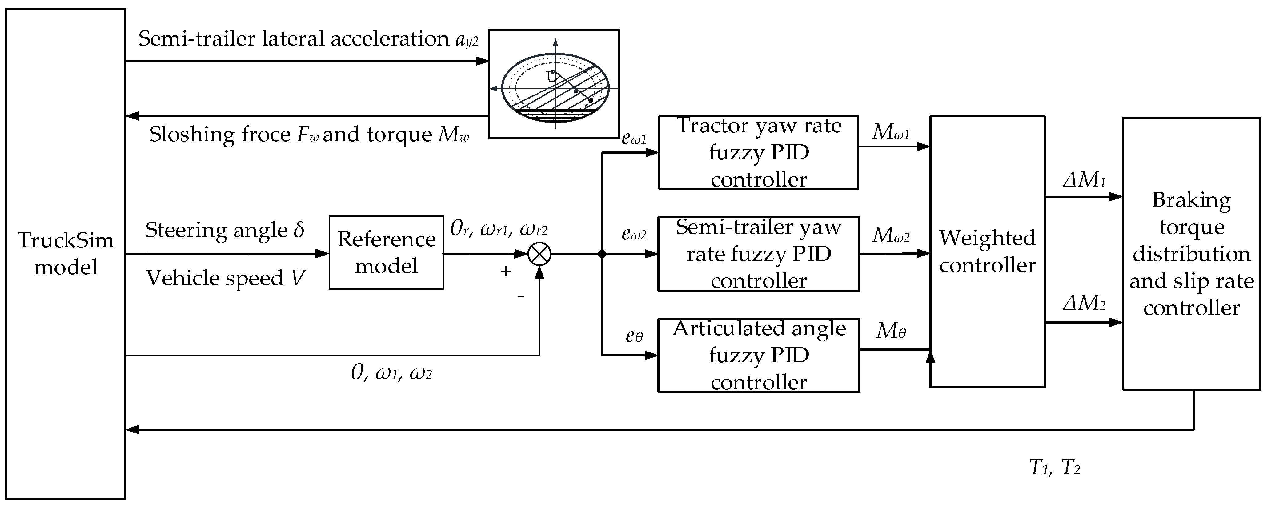
4.1. General Architecture of Yaw Stability Control Method for the Liquid Tank Semi-Trailer

The general architecture of the yaw stability control method for the liquid tank semi-trailer is shown in Figure 7. The TP model calculates the force and torque generated by liquid sloshing, the TruckSim software provides the real-time state parameters of the vehicle, and the reference model provides the expected values of state parameters of the vehicle. The difference between the real-time state parameters and the stable state parameters is controlled by the tractor yaw rate fuzzy PID controller, the semi-trailer yaw rate fuzzy PID controller, and the articulation angle fuzzy PID controller, and the final additional yaw moment required by the tractor and semi-trailer is obtained after the weighted control of the above three. The additional yaw moment of the vehicle is provided by the braking torque of the wheels. Through the braking torque distribution and the wheel slip rate control, the braking torque of each wheel of the tractor and the semi-trailer is fed back to the TruckSim software to correct the state of the vehicle in real-time, to achieve the yaw stability control of the liquid tank semi-trailer.

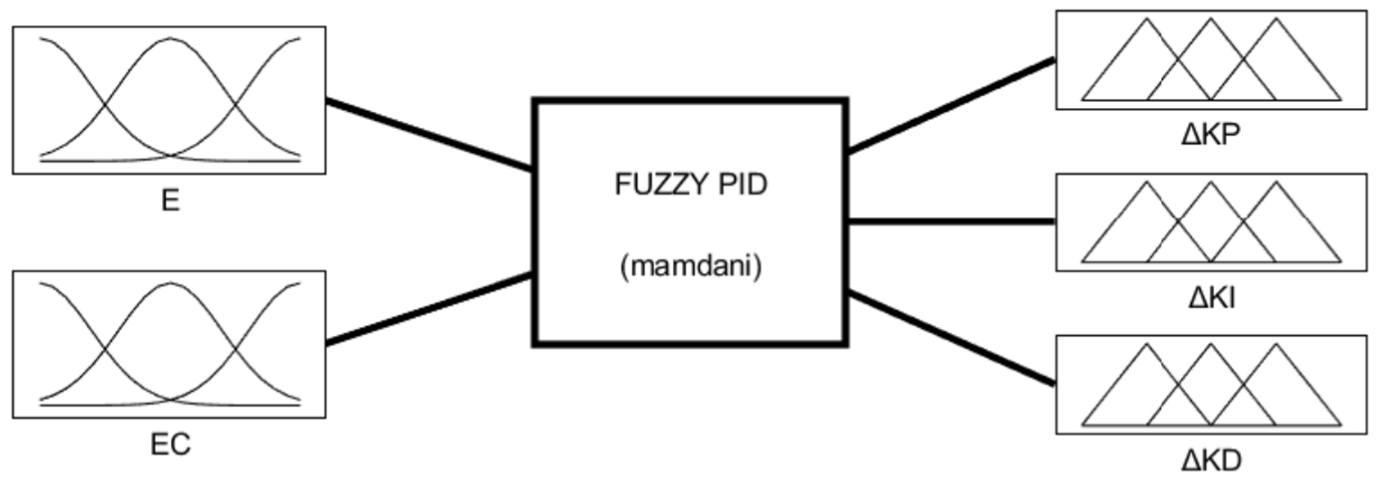
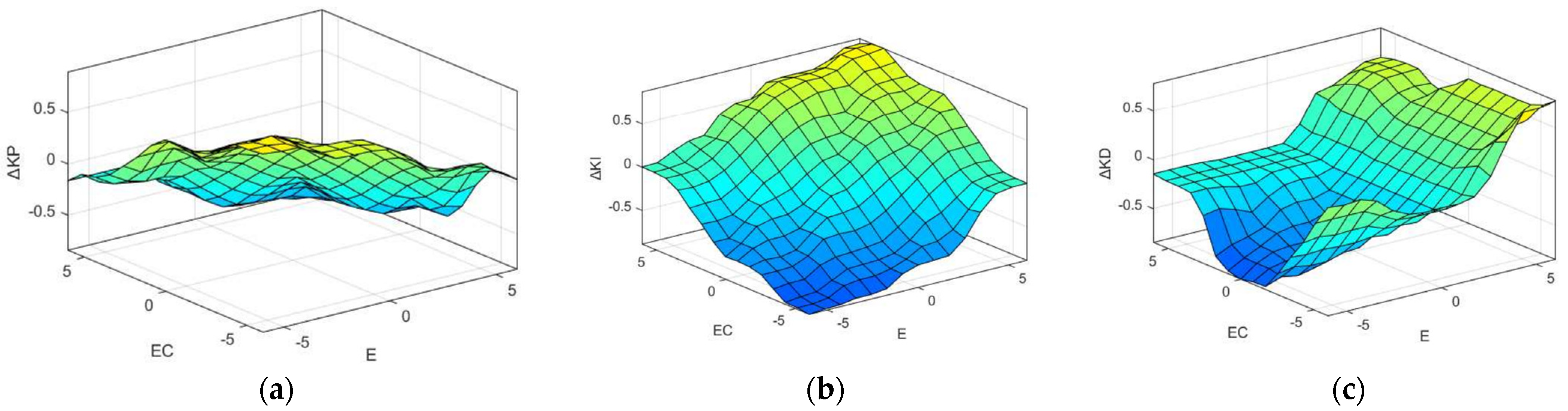
4.2. Calculation of the Additional Yaw Moment of Yaw Stability Control Method for the Liquid Tank Semi-Trailer

Considering the high nonlinearity of the liquid tank semi-trailer model, the fuzzy PID controller with a simple structure and strong robustness is taken to calculate the additional yaw moment required by the tractor and semi-trailer. Its typical structure is shown in Figure 8. The inputs of the fuzzy PID controller are deviation e and deviation change rate e c . The outputs are the increments of the control parameters of the fuzzy PID controller, Δ K P ,   Δ K I ,   Δ K D .
The control parameters of the fuzzy PID controller are
{ K P = K P 0 + Δ K P · k u P K I = K I 0 + Δ K I · k u I K D = K D 0 + Δ K D · k u D
where K P 0 ,   K I 0 ,   K D 0 are the initial values of the parameters of the fuzzy PID controller; Δ K P ,   Δ K I ,   Δ K D are the outputs of the fuzzy controller; k u P ,   k u I ,   k u D are the scale factors of the fuzzy PID controller; and K P ,   K I ,   K D are the actual control values of the controller.
The parameters of the fuzzy PID controller are set as follows: deviation e , deviation change rate e c , and PID parameter variation Δ K P ,   Δ K I ,   Δ K D all adopt the Gaussian membership function. After fuzzification, the fuzzy values of deviation e and deviation change rate e c are [−6,6], while those of the PID parameters Δ K P ,   Δ K I ,   Δ K D are [−1,1].
The language variables are negative big (NB), negative middle (NM), negative small (NS), zero (ZO), positive small (PS), positive middle (PM), and positive big (PB), and the corresponding fuzzy subsets are {NB, NM, NS, ZO, PS, PM, PB}.
Finally, the input and output of the fuzzy PID controller are shown in Figure 9. The surface relationships between the input value and the output value are shown in Figure 10. The fuzzy rules of parameters Δ K P ,   Δ K I ,   Δ K D are shown in Table 3, Table 4 and Table 5.
Through the above analysis, the additional yaw moment provided by the tractor yaw rate fuzzy PID controller M ω 1 , the additional yaw moment provided by the fuzzy PID controller for the yaw rate of the semi-trailer M ω 2 , and the additional yaw moment provided by the articulation angle fuzzy PID controller M θ can be obtained by Equation (21).
{ M ω 1 = K P e ω 1 + K I 0 t e ω 1 d t + K D d e ω 1 d t M ω 2 = K P e ω 2 + K I 0 t e ω 2 d t + K D d e ω 2 d t M θ = K P e θ + K I 0 t e θ d t + K D d e θ d t
Through the weighted control of the three, the additional yaw moment Δ M 1 required by the tractor and the additional yaw moment Δ M 2 required by the semi-trailer can be obtained by Equation (22).
{ Δ M 1 = M ω 1 Δ M 2 = w 1 M ω 2 + w 2 M θ
where w 1 , w 2 are the weight coefficients of the yaw rate controller and the articulation angle controller of the semi-trailer, respectively. After several simulation comparisons, the weight coefficient w 1 is taken as 0.6, and w 2 is taken as 0.4.

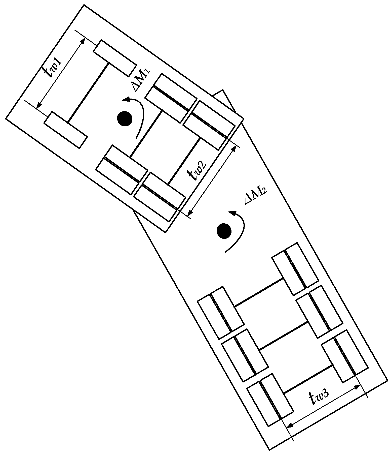
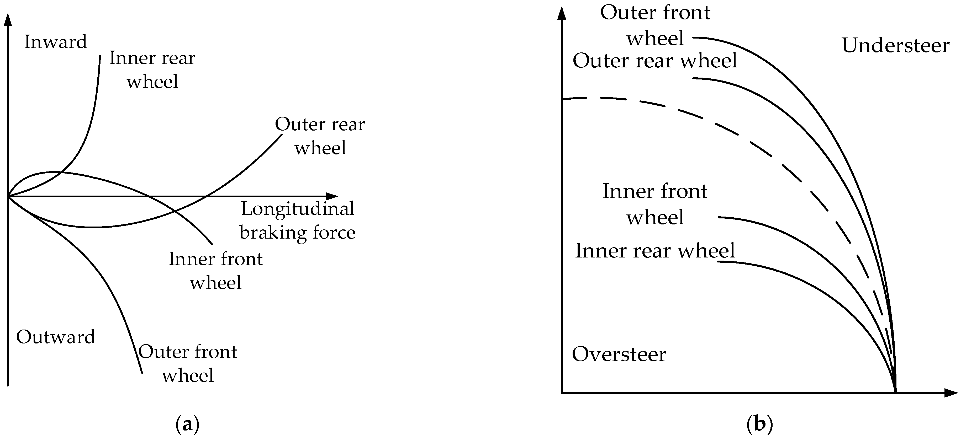
4.3. Calculation and Distribution of Braking Torque of Yaw Stability Control Method for the Liquid Tank Semi-Trailer

When the additional yaw moment required for differential braking of the liquid tank semi-trailer is calculated based on the multi-object PID controller, it is necessary to calculate the braking moment generated by the wheels of the tractor and semi-trailer T 1 , T 2 . The additional yaw moment of the vehicle is provided by the braking force applied to the wheels. Therefore, only by determining the relationship between the additional yaw moment and the braking force of different wheels can the braking torque be accurately calculated. Take the direction in which the vehicle turns left as the positive one and the other as the negative one. The relationship between the additional yaw moment and the braking moment of the liquid tank semi-trailer under the left-turning condition is shown in Figure 11.
In Figure 12, t w 1 , t w 2 ,   t w 3 is the track width of the front axle of the tractor, the second and third axles of the tractor and the fourth, fifth, and sixth axles of the semi-trailer; Δ M 1 , Δ M 2 is the additional yaw moment of the tractor and semi-trailer. When the vehicle performs differential braking, supposing that the braking force is applied to the left wheel of the first axle of the tractor and the left wheels of the fourth, fifth, and sixth axles of the semi-trailer, it can be obtained from the mechanical knowledge that
{ Δ M 1 = F x l 1 · t w 1 2 Δ M 2 = ( F x l 4 + F x l 5 + F x l 6 ) · t w 3 2  
where F x l 1 is the braking force applied to the left wheel of the first axle of the tractor; F x l 4 , F x l 5 , F x l 6 are the braking forces applied to the left wheels of the fourth, fifth, and sixth axles of the semi-trailer, respectively; and t w 1 , t w 3 are the first axle base of the tractor and the fourth, fifth, and sixth axle bases of the semi-trailer, respectively.
The cornering stiffness of the tire will change due to the change in the vertical load of the tire, and the change in the cornering stiffness of the tire will affect the yaw stability of the vehicle. Assuming that the moment of the braking wheel when the tire is not locked is approximately proportional to its vertical load, the braking force applied by the left wheel of the first axle of the tractor and the braking force distribution formula of the left wheel of the fourth, fifth, and sixth axles of the semi-trailer can be expressed, respectively, as follows:
F x f l = 2 Δ M 1 t w 1
{ F x l 4 = F z l 4 F z l 4 + F z l 5 + F z l 6 · 2 Δ M 2 t w 3 F x l 5 = F z l 5 F z l 4 + F z l 5 + F z l 6 · 2 Δ M 2 t w 3 F x l 6 = F z l 6 F z l 4 + F z l 5 + F z l 6 · 2 Δ M 2 t w 3
where F z l 4 , F z l 5 , F z l 6 are the vertical load of the left wheel of the fourth, fifth, and sixth axles of the semi-trailer, respectively.
The braking moment of the left wheel on the first axle of the tractor and the left wheel on the fourth, fifth, and sixth axles of the semi-trailer can be expressed, respectively, as follows:
T l 1 = F x l 1 R 1 = 2 Δ M 1 t w 1 · R 1
{ T l 4 = F x l 4 R 3 = F I l 4 F z l 4 + F z l 5 + F z l 6 · 2 Δ M 2 t w 3 · R 3 T l 5 = F x l 5 R 3 = F z l 5 F z l 4 + F I l 5 + F z l 6 · 2 Δ M 2 t w 3 · R 3 T l 6 = F x l 6 R 3 = F z l 6 F z l 4 + F z l 5 + F z l 6 · 2 Δ M 2 t w 3 · R 3
where R 1 is the wheel rolling radius of the first axle of the tractor; and R 3 is the wheel rolling radius of the fourth, fifth, and sixth axles of the semi-trailer.
From the previous analysis, the additional yaw moment required by the tractor and semi-trailer can be converted into the braking moment of the wheel. After that, the target braking wheel needs to be determined to generate the additional yaw moment efficiently.
As shown in Figure 12a, when the outer front wheels of the vehicle brake, the generated yaw moment gradually increases outwards; when the outer rear wheels of the vehicle brake, the yaw moment produced gradually increases and then decreases outwards, and finally gradually increases inwards; when the inner front wheels of the vehicle brake, the yaw moment generated gradually increases, then decreases inwards, and finally increases outwards; when the inner rear wheels of the vehicle brake, the yaw moment generated gradually increases inwards.
As shown in Figure 12b, when the liquid tank semi-trailer runs in a steady circular motion, the brake of the vehicle’s outer front wheel will cause the vehicle to understeer, and the trend is large; the brake of the vehicle’s outer rear wheel will cause the vehicle to understeer, and the trend is relatively small; the front wheel braking in the vehicle will cause the vehicle to oversteer, and the trend is relatively small; and the rear wheel braking in the vehicle will cause the vehicle to oversteer, and the trend is large.
Based on this, when the outer front wheel and the outer rear wheel of the vehicle brake, the brake efficiency of the outer front wheel is higher under the same conditions; when the inner front wheel and inner rear wheel of the vehicle brake, the brake efficiency of the inner rear wheel is higher under the same conditions [18].
To sum up, the wheel braking moment should be distributed by judging the deviation between the actual value and the expected value of the steering direction and yaw rate, and the deviation between the actual value and the expected value of the articulation angle. The final distribution rules are shown in Table 6.

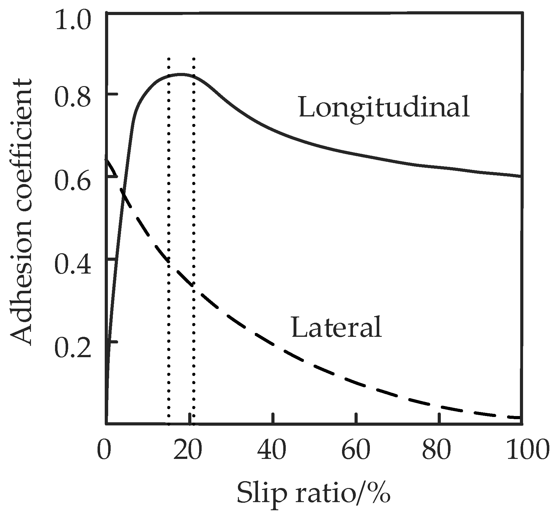
4.4. Wheel Slip Rate Control in Yaw Stability Control Method for the Liquid Tank Semi-Trailer

The calculation formula of the wheel slip ratio is
λ = u r w w u
where u is the longitudinal velocity of the tractor or semi-trailer; r w is the rolling radius of the wheel; and w is the angular velocity of the wheel.
Figure 13 shows that when the slip ratio is 0.15–0.20, the longitudinal adhesion coefficient and lateral adhesion coefficient are both large, and the longitudinal force and lateral force on the tire are also sufficient, so the vehicle can maintain good dynamic performance and stability.
To control the vehicle tire slip rate within 0.15–0.20, when the wheel slip rate is greater than 0.20, the braking torque shall be reduced to reduce the wheel slip rate; when the wheel slip ratio is between 0.15 and 0.20, the braking torque should remain unchanged; when the wheel slip rate is lower than 0.15, the wheel braking torque shall be increased to increase the wheel slip rate. It should be noted that in the process of increasing or decreasing the braking torque, the appropriate growth rate and decline rate should be selected. When the growth rate and decline rate are too large, the slip rate will overshoot and even cause system vibration; when the values of the growth rate and the decline rate are too small, the slip rate changes slowly, and the system response is not sensitive. According to the characteristics of the wheel, the appropriate growth rate and decline rate are selected, and the corresponding braking torque can be obtained
{ T t + 1 = T t + k i T s , S < 0.15 T t + 1 = T t ,     0.15 S 0.2 T t + 1 = T t k d T s , S > 0.2
where T t + 1 is the output value of braking torque at time t + 1 ; T t is the output value of braking torque at time t ; T s is the calculation time interval, 0.005 s; k i is the growth rate, which is 6000   N · m / s ; and k d is decline rate, 6000   N · m / s .

5. Verification of the Effectiveness and Robustness of the Yaw Stability Control Method for the Liquid Tank Semi-Trailer

To verify the effectiveness of the proposed control method, based on the liquid tank semi-trailer co-simulation model, the different vehicle state responses are compared while taking the multi-object PID differential braking-control (multi-object), tractor yaw rate + semi-trailer yaw rate differential braking-control ( ω 1 + ω 2 ), tractor yaw rate + articulation angle differential braking-control ( ω 1 + θ ), and no control methods, respectively. For the verification of the proposed control method, the double-lane change and the step-steering-angle input’s working conditions are selected, the initial vehicle speed is set as 80   km / h , the road adhesion coefficient is set as 0.3, and the basic vehicle parameters can be referred to in Table 2.
To verify the robustness of the proposed method, the robustness of the proposed control method is analyzed and verified when the multi-object PID control parameters are changed.

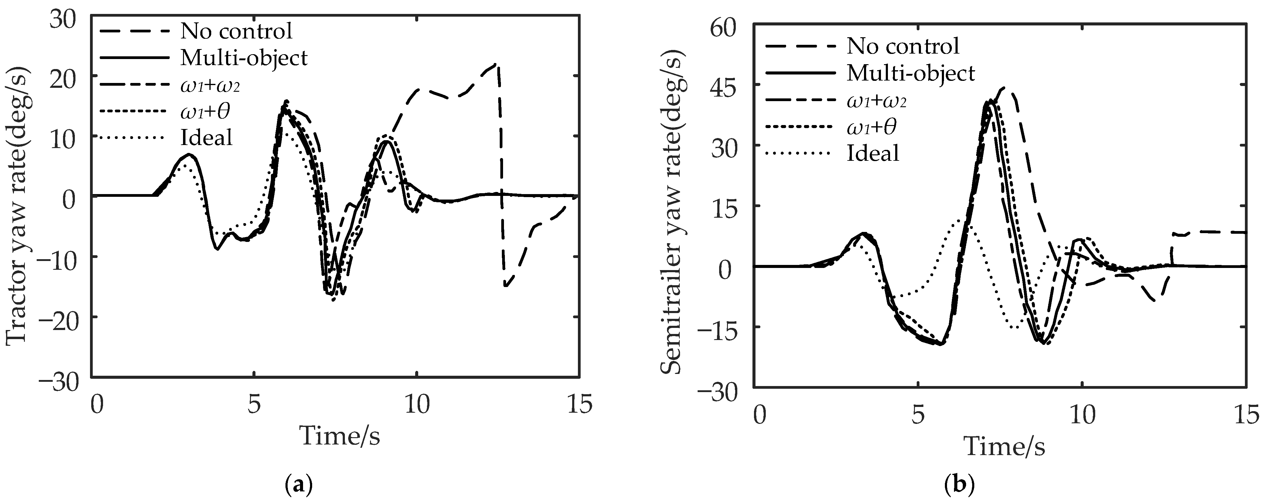
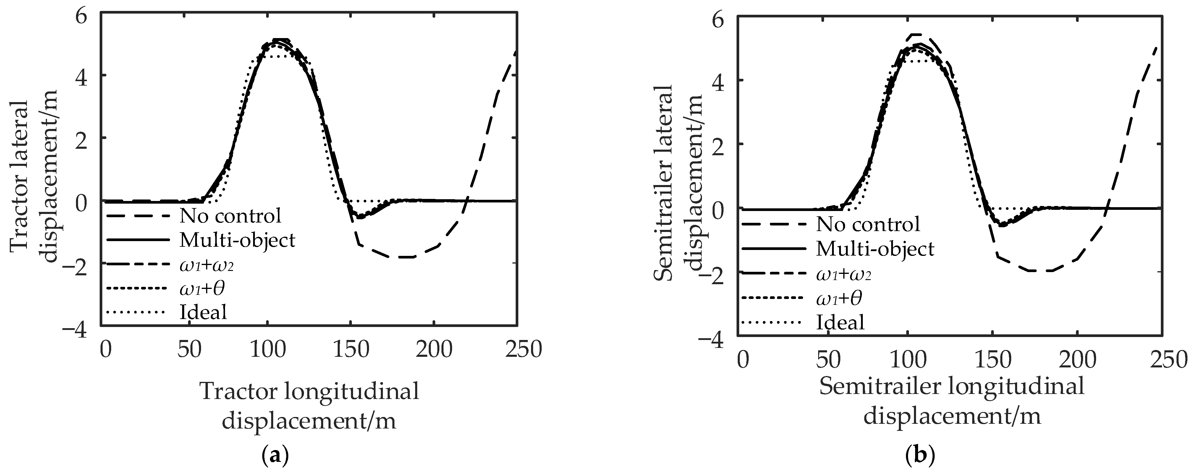
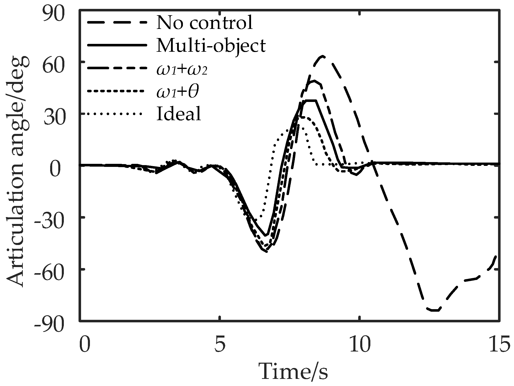
5.1. Verification of the Effectiveness of the Yaw Stability Control Method under the Double-Lane Change Working Condition

In this section, the double-lane change working condition simulation test is performed when the liquid tank semi-trailer is running on a low-adhesion coefficient road. The comparison diagrams of the yaw rate, the vehicle track, and the articulation angle of the tractor and semi-trailer are shown in Figure 14, Figure 15 and Figure 16, respectively.
It can be seen from Figure 14a,b that compared with no control, multi-object control reduces the maximum yaw rate of the tractor by 45.45% and the maximum yaw rate of the semi-trailer by 4.55%; for ω 1 + ω 2 , the maximum yaw rate of the tractor is reduced by 50.15%, and the maximum yaw rate of the semi-trailer is reduced by 6.82%; for ω 1 + θ , the control reduces the maximum yaw rate of the tractor by 40.91%, and the maximum yaw rate of the semi-trailer by 2.27%. In conclusion, compared with the no control strategy, the multi-object control and ω 1 + ω 2 control can effectively reduce the maximum yaw rate of the tractor and semi-trailer.
It can be seen from Figure 15 and Figure 16 that compared with no control, the maximum lateral displacement deviation of the tractor under multi-object control is reduced by 3.71%, the maximum lateral displacement deviation of the semi-trailer is reduced by 5.45%, and the maximum articulation angle is reduced by 46.67%; for ω 1 + ω 2 control, the lateral displacement deviation of the tractor, semi-trailer, and the maximum articulation angle are reduced by 1.85%, 3.64%, and 33.33%, respectively; the ω 1 + θ control reduced the lateral displacement deviation of the tractor by 5.56%, the lateral displacement deviation of the semi-trailer by 7.28%, and the maximum articulation angle by 58.33%. In conclusion, compared with the no control strategy, the multi-object control and ω 1 + θ control can effectively reduce the maximum lateral displacement deviation and articulation angle of the tractor and semi-trailer.

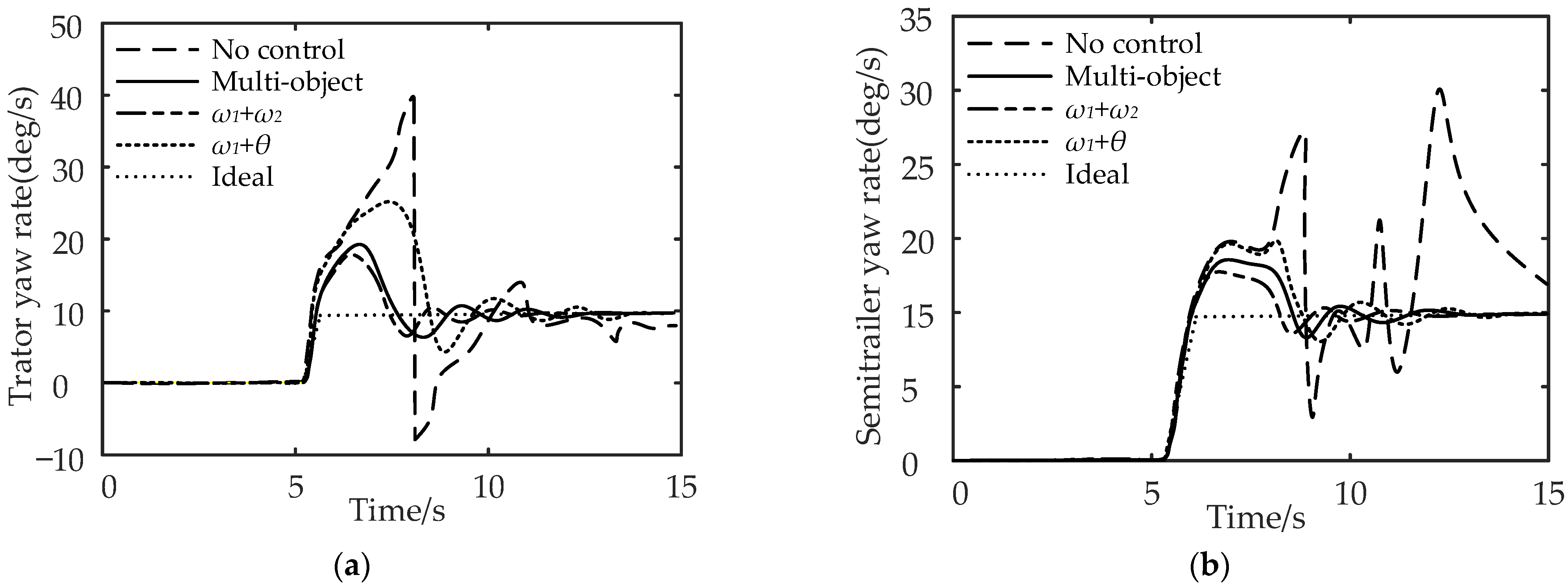
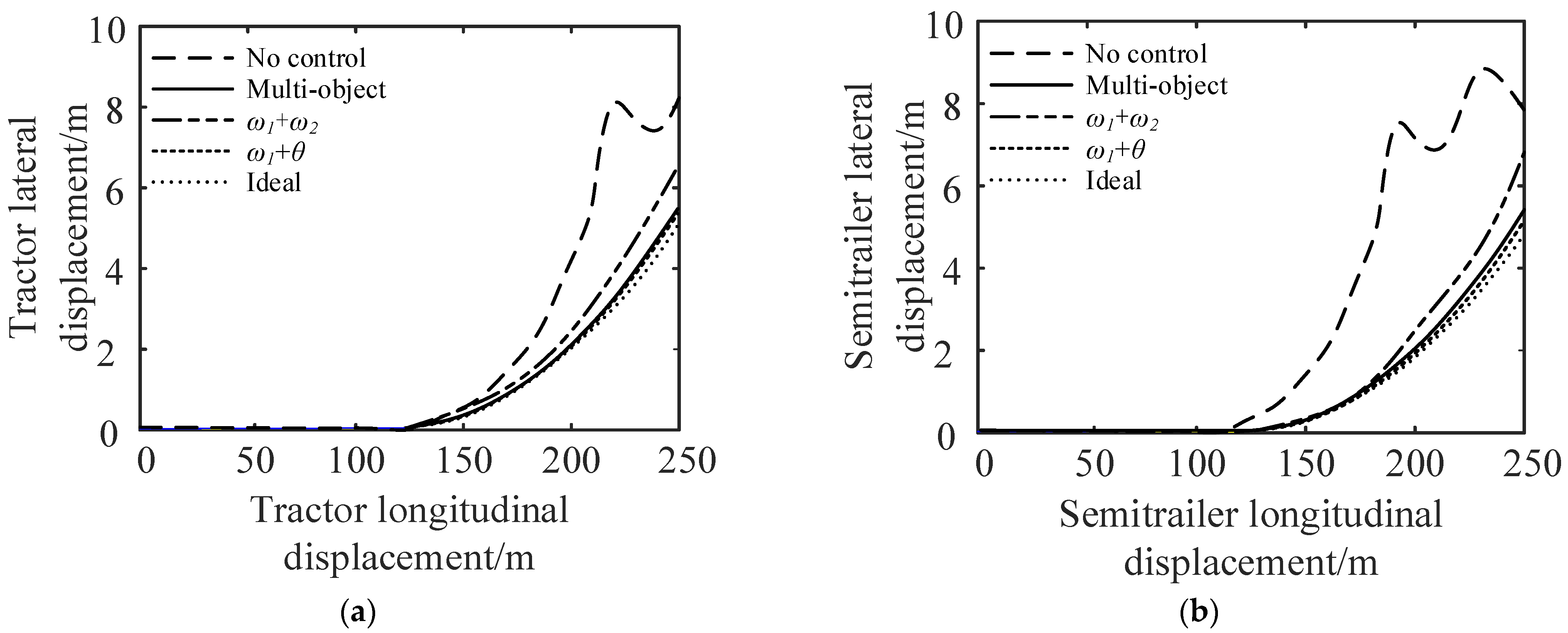
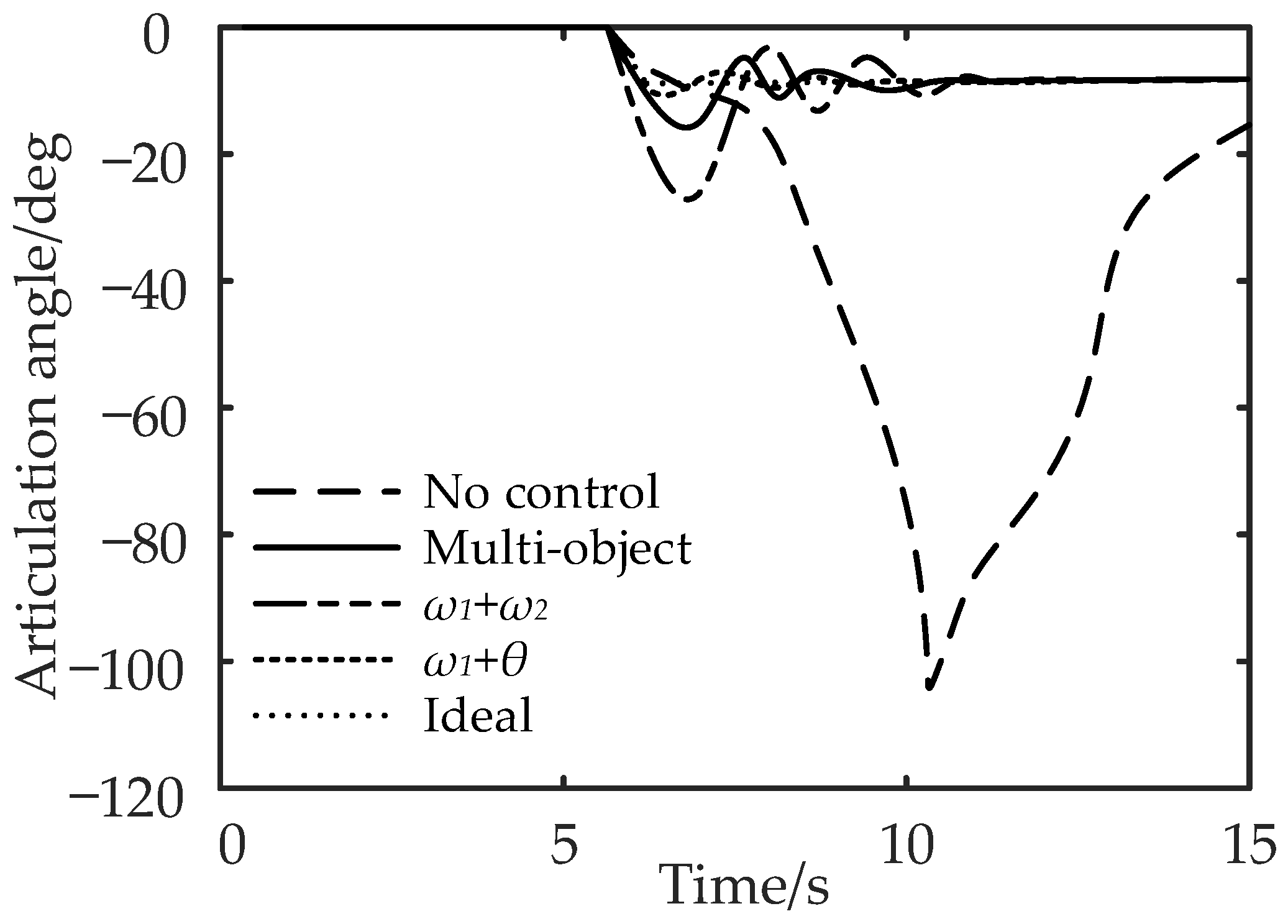
5.2. Verification of the Effectiveness of the Yaw Stability Control Method under the Step-Steering-Angle Input Working Condition

In this section, the step-steering-angle input working condition simulation test is per-formed when the liquid tank semi-trailer is running on a low-adhesion coefficient road. The comparison diagrams of the yaw rate, the vehicle track, and the articulation angle of the tractor and semi-trailer are shown in Figure 17, Figure 18 and Figure 19, respectively.
It can be seen from Figure 17a,b that compared with no control, multi-object control reduces the maximum yaw rate of the tractor by 52.5% and the maximum yaw rate of the semi-trailer by 43.3%; for ω 1 + ω 2 , the maximum yaw rate of the tractor is reduced by 57.5%, and the maximum yaw rate of the semi-trailer is reduced by 46.7%; for ω 1 + θ , the control reduces the maximum yaw rate of the tractor by 37.5%, and the maximum yaw rate of the semi-trailer by 36.7%. In conclusion, compared with the no control strategy, the multi-object control and ω 1 + ω 2 control can effectively reduce the maximum yaw rate of the tractor and semi-trailer.
It can be seen from Figure 18 and Figure 19 that compared with no control, the maximum lateral displacement deviation of the tractor under multi-object control is reduced by 31.3%, the maximum lateral displacement deviation of the semi-trailer is reduced by 38.9%, and the maximum articulation angle is reduced by 81.5%; for ω 1 + ω 2 control, the lateral displacement deviation of the tractor, semi-trailer, and the maximum articulation angle are reduced by 25.3%, 33.3%, and 25.5% respectively; the ω 1 + θ control reduced the lateral displacement deviation of the tractor by 37.5%, the lateral displacement deviation of the semi-trailer by 42.2%, and the maximum articulation angle by 88.2%. In conclusion, compared with the no control strategy, the multi-object control and ω 1 + θ control can effectively reduce the maximum lateral displacement deviation and articulation angle of the tractor and semi-trailer.
To sum up, compared with the differential braking control aiming at the yaw rate or articulation angle of the tractor, the multi-object PID differential braking control can not only improve the yaw stability of the semi-trailer turning on the low-adhesion road but also improve the path-following performance.

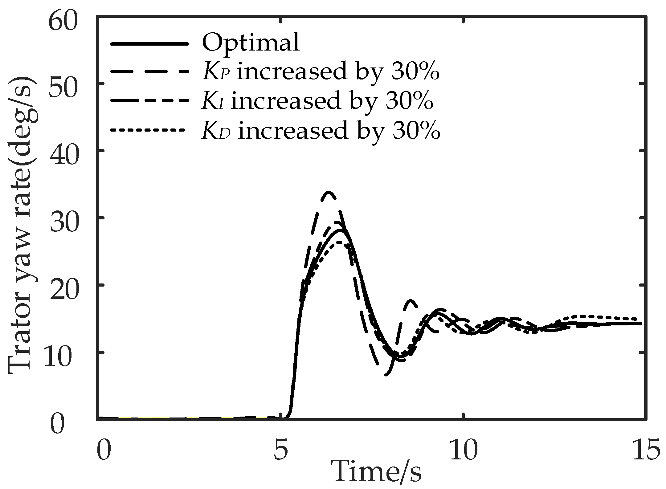
5.3. Verification of the Robustness of the Yaw Stability Control Method

The effectiveness of the proposed control method in controlling the vehicle yaw stability is verified in the previous two sections. As another important criterion to evaluate the quality of the control system, the robustness of the proposed control method is analyzed and verified.
The robustness of control system means that the system has the ability to maintain a certain performance under the disturbance of uncertainty [19]. The proposed multi-objective PID control method is established based on the fuzzy PID control method, which has good stability and robustness [20]. To verify the robustness of the proposed control method, the tractor yaw rates under the step-steering-angle input working condition are compared when the control parameters K P , K I , and K D of the multi-object PID control method are increased by 30%. The other simulation parameters are the same with those in Section 5.2, and the comparison results are shown in Figure 20.
It can be seen from Figure 20 that compared with the control effect of the optimal parameters, the differences between the tractor yaw rate curves are not significant when these three parameters K P , K I , and K D are increased by 30%, which proves the robustness of the proposed control method.

6. Conclusions

(1)
The TP model is established to simulate the sloshing effect of the liquid in the elliptical cylinder tank under lateral excitation, and its simulation effect is validated using the Fluent software. Based on it, a co-simulation model is established based on TruckSim and MATLAB/Simulink.
(2)
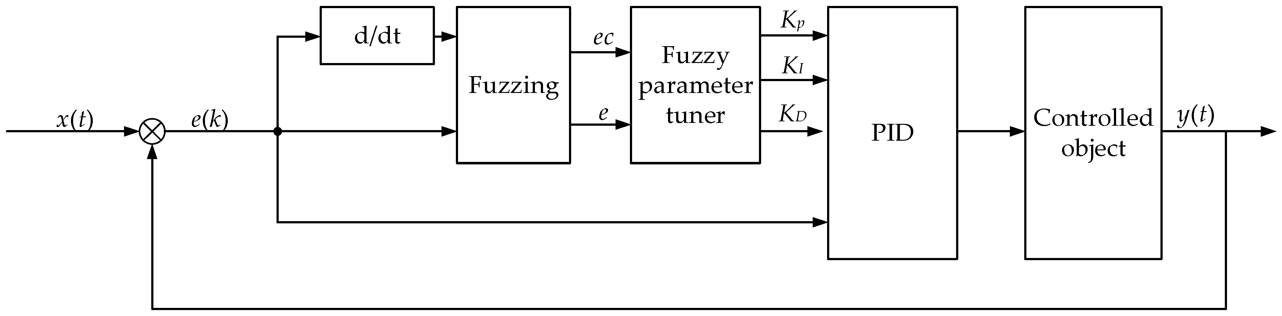
A simplified six degrees of freedom model of the liquid tank semi-trailer is established and verified using the TruckSim software. Taking the tractor yaw rate, semi-trailer yaw rate, and articulation angle as the control parameters, a multi-object PID differential braking-control method is proposed and implemented.
(3)
The vehicle state responses with and without control are compared under the double-lane change and the step-steering-angle input working conditions on a low-adhesion road. The simulation results show that, compared with the differential braking control, which targets the yaw rate or articulation angle of the tractor, the multi-object PID differential braking control can not only improve the yaw stability of the vehicle but also improve the path-following performance of the semi-trailer.

Author Contributions

Conceptualization, G.L. and T.F.; methodology, T.F. and G.L.; software, T.F. and R.Z.; validation, G.L., R.Z. and T.F.; formal analysis, T.F. and R.Z.; investigation, T.F. and R.Z.; resources, G.L.; data curation, T.F.; writing—original draft preparation, T.F.; writing—review and editing, T.F., G.L. and R.Z.; visualization, T.F. and G.L.; supervision, G.L. and R.Z.; project administration, G.L.; funding acquisition, G.L. All authors have read and agreed to the published version of the manuscript.

Funding

This research was funded by the China Postdoctoral Science Foundation, grant number 2018M642937, which is a cooperation with the SMC Corporation.

Institutional Review Board Statement

Not applicable.

Informed Consent Statement

Not applicable.

Data Availability Statement

The study did not report any data.

Acknowledgments

Thanks to Gangyan Li and Ran Zhao of Wuhan University of Technology for supporting and helping this study.

Conflicts of Interest

The authors declare no conflict of interest.

References

  1. Zhao, R.; Li, G.; Yu, B.; Yang, F. The brake pressure change rate in brake chamber and its online monitoring in semitrailer transport vehicle for dangerous cargo. Proc. Inst. Mech. Eng. Part D J. Automob. Eng. 2022. Available online: https://journals.sagepub.com/doi/abs/10.1177/09544070221091684 (accessed on 20 April 2022). [CrossRef]
  2. Zheng, H.; Hu, J.; Ma, S. Research on Simulation and Control of Differential Braking Stability of Tractor Semi-Trailer. SAE Tech. Pap. 2015. [CrossRef]
  3. Li, X.-S.; Zheng, X.-L.; Ren, Y.-Y.; Wang, Y.-N.; Cheng, Z.-Q. Study on Driving Stability of Tank Trucks Based on Equivalent Trammel Pendulum for Liquid Sloshing. Discret. Dyn. Nat. Soc. 2013, 2013, 659873–659887. [Google Scholar] [CrossRef] [Green Version]
  4. Peng, G.; Zhao, Z.; Liu, T.; Hu, H.; Feng, M. Research on Dynamic Characteristics of Lateral Sloshing in Liquid Tank Semi-Trailer. In Proceedings of the 2019 3rd Conference on Vehicle Control and Intelligence (CVCI), Hefei, China, 21–22 September 2019; pp. 1–6. [Google Scholar] [CrossRef]
  5. Saeedi, M.A.; Kazemi, R.; Azadi, S. Improvement in the rollover stability of a liquid-carrying articulated vehicle via a new robust controller. Proc. Inst. Mech. Eng. Part D J. Automob. Eng. 2017, 231, 322–346. [Google Scholar] [CrossRef]
  6. Dewangan, D.K.; Sahu, S.P. Real Time Object Tracking for Intelligent Vehicle. In Proceedings of the 2020 First International Conference on Power, Control and Computing Technologies (ICPC2T), Raipur, India, 3–5 January 2020; pp. 134–138. [Google Scholar] [CrossRef]
  7. Celebi, M.; Akyildiz, H. Nonlinear modeling of liquid sloshing in a moving rectangular tank. Ocean Eng. 2002, 29, 1527–1553. [Google Scholar] [CrossRef]
  8. Salem, M.I.; Mucino, V.H.; Saunders, E.; Gautam, M.; Guzman, A.L. Lateral sloshing in partially filled elliptical tanker trucks using a trammel pendulum. Int. J. Heavy Veh. Syst. 2009, 16, 207–224. [Google Scholar] [CrossRef]
  9. Salem, M.I. Rollover Stability of Partially Filled Heavy-Duty Elliptical Tankers Using Trammel Pendulums to Simulate Fluid Sloshing; West Virginia University: Morgantown, WV, USA, 2000. [Google Scholar]
  10. Bai, Z.; Lu, Y.; Li, Y. Method of Improving Lateral Stability by Using Additional Yaw Moment of Semi-Trailer. Energies 2020, 13, 6317. [Google Scholar] [CrossRef]
  11. Zhao, C.; Xiang, W.; Richardson, P. Vehicle Lateral Control and Yaw Stability Control through Differential Braking. In Proceedings of the 2006 IEEE International Symposium on Industrial Electronics, Montreal, QC, Canada, 9–13 July 2006; Volume 1, pp. 384–389. [Google Scholar] [CrossRef]
  12. Zhou, H.; Liu, Z. Vehicle Yaw Stability-Control System Design Based on Sliding Mode and Backstepping Control Approach. IEEE Trans. Veh. Technol. 2010, 59, 3674–3678. [Google Scholar] [CrossRef]
  13. Xue-Lian, Z.; Xian-Sheng, L.; Yuan-Yuan, R. Equivalent Mechanical Model for Lateral Liquid Sloshing in Partially Filled Tank Vehicles. Math. Probl. Eng. 2012, 2012, 162825–162846. [Google Scholar] [CrossRef] [Green Version]
  14. Xiu-jian, Y.; Yun-xiang, X.; Xiang-ji, W.U.; Kun, Z. Multi-Mass Trammel Pendulum Model of Fluid Lateral Sloshing for Tank Vehicle. J. Traffic Transp. Eng. 2018, 18, 140–151. [Google Scholar] [CrossRef]
  15. Wan, Y.; Mai, L.; Nie, Z.G. Dynamic Modeling and Analysis of Tank Vehicle under Braking Situation. Adv. Mater. Res. 2013, 694, 176–180. [Google Scholar] [CrossRef]
  16. Cai, H.; Xu, X. Lateral Stability Control of a Tractor-Semitrailer at High Speed. Machines 2022, 10, 716. [Google Scholar] [CrossRef]
  17. Xu, X.; Zhang, L.; Jiang, Y.; Chen, N. Active Control on Path Following and Lateral Stability for Truck–Trailer Combinations. Arab. J. Sci. Eng. 2019, 44, 1365–1377. [Google Scholar] [CrossRef]
  18. Her, H.; Koh, Y.; Joa, E.; Yi, K.; Kim, K. An Integrated Control of Differential Braking, Front/Rear Traction, and Active Roll Moment for Limit Handling Performance. IEEE Trans. Veh. Technol. 2015, 65, 4288–4300. [Google Scholar] [CrossRef]
  19. Sariyildiz, E.; Ohnishi, K. Stability and Robustness of Disturbance-Observer-Based Motion Control Systems. IEEE Trans. Ind. Electron. 2014, 62, 414–422. [Google Scholar] [CrossRef] [Green Version]
  20. Duan, X.-G.; Li, H.-X.; Deng, H. Robustness of fuzzy PID controller due to its inherent saturation. J. Process Control 2012, 22, 470–476. [Google Scholar] [CrossRef]
Figure 1. Schematic diagram of the TP model.
Applsci 13 00039 g001
Figure 2. Comparison of liquid sloshing results: (a) sloshing force and (b) sloshing torque between Fluent software and the TP model.
Applsci 13 00039 g002
Figure 3. Schematic diagram of co-simulation model for liquid tank semi-trailer.
Applsci 13 00039 g003
Figure 4. TruckSim I/O setting module: (a) input module and (b) output module.
Applsci 13 00039 g004
Figure 5. Schematic diagram of the liquid tank semi-trailer: (a) XOY plane diagram, (b) tractor roll model, and (c) semi-trailer roll model.
Applsci 13 00039 g005
Figure 6. Comparison of vehicle state responses between simplified model and TruckSim model: (a) comparison of yaw rate of the tractor and (b) comparison of articulation angle.
Applsci 13 00039 g006
Figure 7. The general architecture of the multi-object PID differential braking-control method.
Applsci 13 00039 g007
Figure 8. Structure of fuzzy PID controller.
Applsci 13 00039 g008
Figure 9. Input and output of the fuzzy controller.
Applsci 13 00039 g009
Figure 10. Fuzzy PID output surface relationships: (a) Δ K P output surface, (b) Δ K I output surface, and (c) Δ K D output surface.
Applsci 13 00039 g010
Figure 11. Relationship between additional yaw moment and braking torque of liquid tank semi-trailer.
Applsci 13 00039 g011
Figure 12. Braking characteristics of different brake wheels: (a) relationship between yaw moment generated by braking of different wheels and longitudinal braking force and (b) influence of single wheel braking on vehicle steering.
Applsci 13 00039 g012
Figure 13. Relationship between longitudinal and lateral adhesion coefficient and slip ratio.
Applsci 13 00039 g013
Figure 14. Comparison of vehicle yaw rate under the double-lane change working condition: (a) comparison of tractor yaw rate and (b) comparison of semi-trailer yaw rate.
Applsci 13 00039 g014
Figure 15. Comparison of vehicle track under the double-lane change working condition: (a) comparison of tractor track and (b) comparison of semi-trailer track.
Applsci 13 00039 g015
Figure 16. Comparison of articulation angle under the double-lane change working condition.
Applsci 13 00039 g016
Figure 17. Comparison of vehicle yaw rate under the step-steering-angle input working condition: (a) comparison of tractor yaw rate and (b) comparison of semi-trailer yaw rate.
Applsci 13 00039 g017
Figure 18. Comparison of vehicle track under the step-steering-angle input working condition: (a) comparison of tractor track and (b) comparison of semi-trailer track.
Applsci 13 00039 g018
Figure 19. Comparison of articulation angle under the step-steering-angle input working condition.
Applsci 13 00039 g019
Figure 20. Comparison of the tractor yaw rates under the step-steering-angle input working condition when the control parameters K P , K I , and K D of the multi-object PID control method are increased by 30%.
Applsci 13 00039 g020
Table 1. Description and value of TP model parameters and basic parameters of the tank.
Parameter DescriptionValueUnit
l a p long semi-axes of the motion track of the pendulum ball 0.5613 m
l b p short semi-axes of the motion track of the pendulum ball 0.3742 m
l a c g long semi-axes of the liquid center of mass motion track m
l b c g short semi-axes of the liquid center of mass motion track m
l a long semi-axes of the tank body section 1.0925 m
l b short semi-axes of the tank body section 0.7283 m
l b s distance from the centroid of the liquid at rest to the bottom of the tank 0.6939 m
m s mass of the liquid at rest 5631 kg
m p mass of the swing ball 7826 kg
m w total mass of liquid in the tank 13 , 457 kg
ζ ellipticity of the section of the liquid tank 1.5
γ liquid swing angle °
Δ liquid filling ratio in the tank 0.6
L tank body length 9 m
ρ liquid density in the tank 997 kg / m 3
a y lateral excitation of the tank body1 m / s 2
Table 2. Basic parameters of the liquid tank semi-trailer.
Parameter Value UnitParameter Value Unit
m 1 5876 kg m 1 s 4457 kg
m 2 25 , 876 kg m 2 s 20 , 000 kg
a 2 m b 2.478 m
c 2.189 m d 4.693 m
e 5.4 m h 1 1.175 m
h 2 2.125 m h 1 c 1.1 m
h 2 c 1.1 m I 1 x x 2283 kg · m 2  
I 1 y y 35 , 402 kg · m 2 I 1 z z 34 , 802 kg · m 2
I 1 x z 1626 kg · m 2 I 2 x x 22 , 330 kg · m 2
I 2 z z 250 , 416 kg · m 2 I 2 x z 0 kg · m 2
Table 3. Fuzzy rule table of Δ K p .
Δ K p
e c
NBNMNSZOPSPMPB
eNBPBPBPMPMPSZOZO
NMPBPBPMPSPSZONS
NSPMPMPMPSZONSNS
ZOPMPMPSZONSNMNM
PSPSPSZONSNSNMNM
PMPSZONSNMNMNMNB
PBZOZONMNMNMNBNB
Table 4. Fuzzy rule table of Δ K I .
Δ K I
e c
NBNMNSZOPSPMPB
eNBNBNBNMNMNSZOZO
NMNBNBNMNSNSZOZO
NSNBNMNSNSZOPSPS
ZONMNMNSZOPSPMPM
PSNMNSZOPSPSPMPB
PMZOZOPSPSPMPBPB
PBZOZOPSPMPMPBPB
Table 5. Fuzzy rule table of Δ K D .
Δ K D
e c
NBNMNSZOPSPMPB
eNBPSNSNBNBNBNMPS
NMPSNSNBNMNMNSZO
NSZONSNMNMNSNSZO
ZOZONSNSNSNSNSZO
PSZOZOZOZOZOZOZO
PMPBPSPSPSPSPSPB
PBPBPMPMPMPSPSPB
Table 6. Rules for wheel braking moment distribution.
Front Wheel Angle δ Tractor/Semi-TrailerControl Parameter DeviationSteering CharacteristicsTarget Brake Wheel
ω r 1 , ω r 2 ω 1 , ω 2 e 1 = ω r 1 ω 1
e 2 = ω r 2 ω 2
e θ = θ r θ
TractorSemitrailer
++++UndersteerL2, L3L4, L5, L6
+++0\\\
+++-OversteerR1R4, R5, R6
++0+UndersteerL2, L3L4, L5, L6
++-+UndersteerL2, L3L4, L5, L6
00+-OversteerR1R4, R5, R6
00-+OversteerL1L4, L5, L6
0000\\\
--+-UndersteerR2, R3R4, R5, R6
--0-UndersteerR2, R3R4, R5, R6
---+OversteerL1L4, L5, L6
---0\\\
----UndersteerR2, R3R4, R5, R6
Note 1: “+”, “-”, “0”, and “\” in the table represent “positive”, “negative”, “0”, and “no control action”, respectively. Note 2: “L1, R1” in the table refer to the left and right wheels of the tractor steering axle; “L2, R2, L3, R3” refer to the left and right wheels of the drive axles of the tractor; “L4, R4, L5, R5, L6, R6” refer to the left and right wheels of the semi-trailer axles.
Disclaimer/Publisher’s Note: The statements, opinions and data contained in all publications are solely those of the individual author(s) and contributor(s) and not of MDPI and/or the editor(s). MDPI and/or the editor(s) disclaim responsibility for any injury to people or property resulting from any ideas, methods, instructions or products referred to in the content.

