
Stock Price Prediction Using a Frequency Decomposition Based GRU Transformer Neural Network

Abstract
:1. Introduction
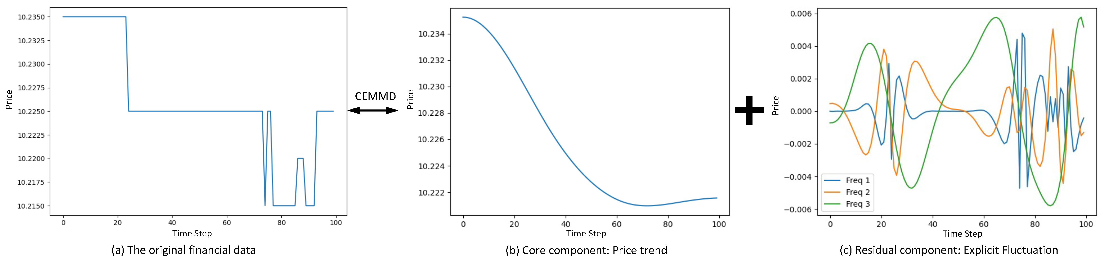
- We decompose the feature of sequential prices into 4 series using CEEMD. After applying CEEMD, there are 1 trend component and 3 mode components, which are far more inofrmative and greatly alleviates the model training problems caused by subtle change problem. Hence, it is well designed for the highly noisy stock data.
- In the FDG-Trans hybrid network structure, transformer is used first to extract fine-grained information between different time steps, followed by LSTM and GRU to do further analysis. This architecture does a well trade-off between capturing more information and reducing overfitting.
- When applied to high frequency data such as limit order book (LOB), FDG-Trans distinguishes the timely variant features such as prices and volumes and timely invariant features such as open price and yesterday close price. In FDG-Trans, the invariant features will not be put into the RNN networks, which further reduces the overfitting and makes the training process more efficient.
2. Related Work
2.1. LSTM Based Models
2.2. GRU Based Models
2.3. Attention Based Models
3. Methods
3.1. Problem Statement
3.2. Problem Analysis and Overview
3.3. Complete Ensemble Empirical Mode Decomposition with Adaptive Noise (CEEMD)
3.3.1. Empirical Mode Decomposition (EMD)
- (1)
- Mark all the local minimums and maximums in the series data .
- (2)
- Apply cubic spline method to determine the lower and upper envelops along the time line.
- (3)
- Obtain the local mean according to the lower and upper envelops.
- (4)
- , if the variance of is less than a pre-defined threshold, then . Otherwise, replace by and repeat the above steps.
- (5)
- , repeat the above process to get . The value of K is determined by the termination condition.
- (6)
- In sum, we get where is a term to indicate the overall trend of series.
3.3.2. Ensemble Empirical Mode Decomposition (EEMD)
3.3.3. Complete Ensemble Empirical Mode Decomposition (CEEMD)
- (1)
- , where is a white noise series. Decompose by EMD to get .
- (2)
- .
- (3)
- Let . Decompose by EMD to get , then
- (4)
- Repeat the above process K steps. For each , , , where is a bunch of noise series, with the variance decreasing in general.
- (5)
- , where K is determined by a pre-defined stopping criteria.
3.4. Hybrid GRU-Transformer
3.4.1. RNN
- : the hidden state at time t
- : the output state at time t
- : the input state at time t
- U: the weight matrix from input layer to hidden layer
- W: the value of the previous hidden layer is used as the weight matrix for the input of the next layer
- V: the weight matrix from hidden layer to output layer
- f: the activation function, usually nonlinear
3.4.2. LSTM and GRU
- : the input gate at time t
- : the forget gate at time t
- : the candidate memory state at time t
- : the memory state at time t
- : the hidden state at time t
- : the output gate at time t
- : the activation function
- : the wight matrix from state x to state y, where i, g, f, h, n mean the input state, the candidate memory state, the forget state, the hidden state, the new memory state, respectively
- : the bias term from state x to state y
- : the update gate at time t
- : the reset gate at time t
- : the new memory state at time t
- : the hidden state at time t
- : the activation function
- : the wight matrix from state x to state y, where i, z, h, n mean the input state, the update state, the hidden state, the new memory state, respectively.
- : the bias term from state x to state y
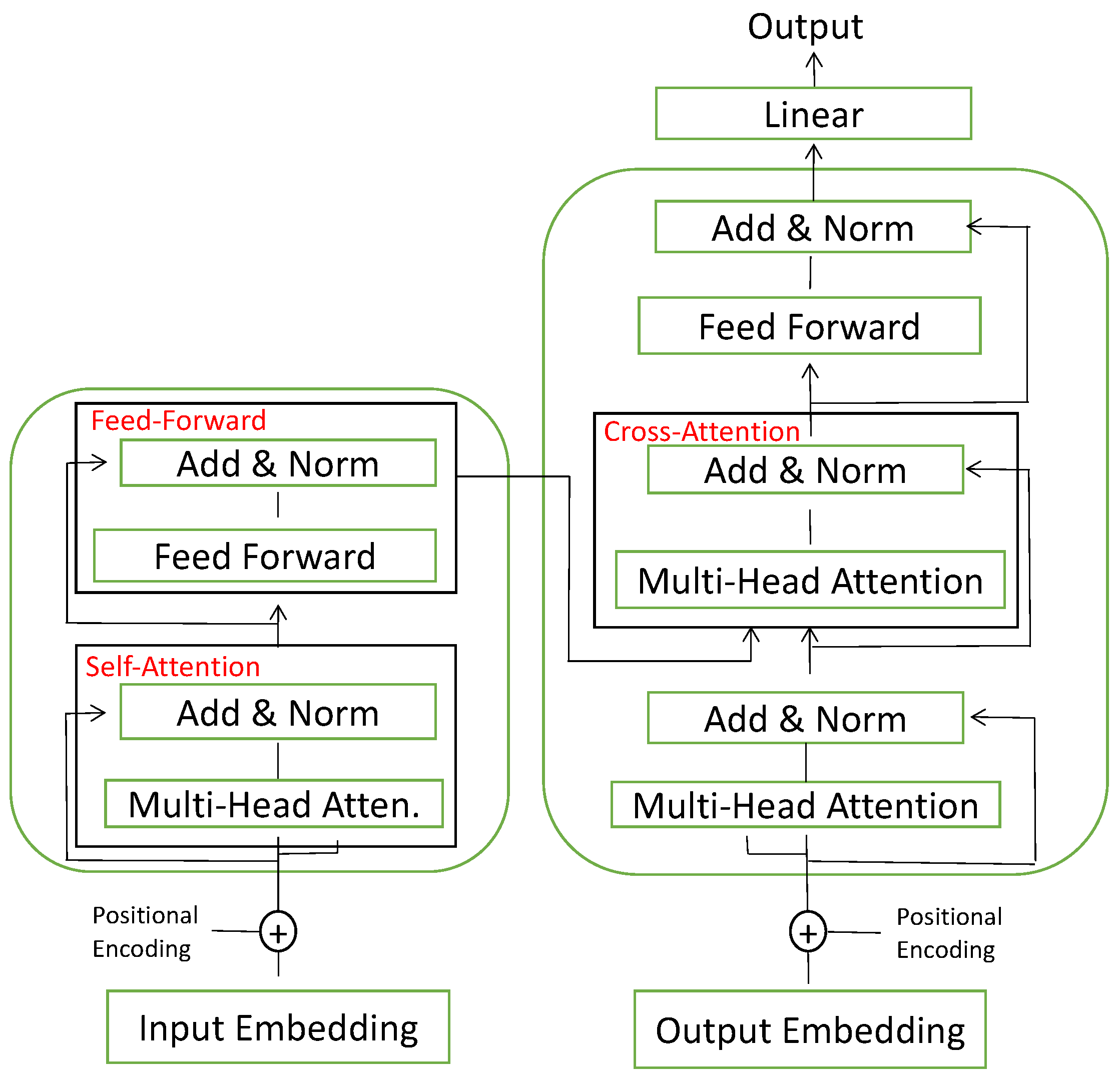
3.4.3. Transformer
3.5. Training Objective
- Mean Absolute Error (MAE):
- Mean Squared Error (MSE):
- Root Mean Squared Error (RMSE):
- Huber Loss:where y is the real value, is the predicted value, n is the number of samples, is a pre-defined threshold.
4. Experiment
4.1. Dataset
4.1.1. Limit Order Book (LOB)
4.1.2. CSI-300
4.2. Evaluation Criterion
4.3. Implementation Details
4.3.1. FDG-Trans
4.3.2. Baseline Method
4.4. Experiment Results
4.4.1. Comparison with the State-of-the-Art Method
4.4.2. Comparison with Baseline Frequency Decomposition
4.4.3. Ablation Study
4.4.4. Visualization of Mode Decomposition
5. Discussion
6. Conclusions
Author Contributions
Funding
Acknowledgments
Conflicts of Interest
References
- Thakkar, A.; Chaudhari, K. Fusion in stock market prediction: A decade survey on the necessity, recent developments, and potential future directions. Inf. Fusion 2021, 65, 95–107. [Google Scholar] [CrossRef]
- Idrees, S.M.; Alam, M.A.; Agarwal, P. A Prediction Approach for Stock Market Volatility Based on Time Series Data. IEEE Access 2019, 7, 17287–17298. [Google Scholar] [CrossRef]
- Rasekhschaffe, K.C.; Jones, R.C. Machine learning for stock selection. Financ. Anal. J. 2019, 75, 70–88. [Google Scholar] [CrossRef]
- Wong, C.S.; Li, W.K. On a mixture autoregressive model. J. R. Stat. Soc. Ser. B 2000, 62, 95–115. [Google Scholar] [CrossRef]
- Hassan, M.R.; Nath, B. Stock market forecasting using hidden Markov model: A new approach. In Proceedings of the 5th International Conference on Intelligent Systems Design and Applications (ISDA’05), Wroclaw, Poland, 8–10 September 2005; pp. 192–196. [Google Scholar]
- Ampomah, E.K.; Qin, Z.; Nyame, G. Evaluation of tree-based ensemble machine learning models in predicting stock price direction of movement. Information 2020, 11, 332. [Google Scholar] [CrossRef]
- Yu, X.; Li, D. Important trading point prediction using a hybrid convolutional recurrent neural network. Appl. Sci. 2021, 11, 3984. [Google Scholar] [CrossRef]
- Picon Ruiz, A.; Alvarez Gila, A.; Irusta, U.; Echazarra Huguet, J. Why deep learning performs better than classical machine learning? Dyna Ing. Ind. 2020. [Google Scholar] [CrossRef] [Green Version]
- Liu, J.; Guo, X.; Li, B.; Yuan, Y. COINet: Adaptive Segmentation with Co-Interactive Network for Autonomous Driving. In Proceedings of the 2021 IEEE/RSJ International Conference on Intelligent Robots and Systems (IROS), Prague, Czech Republic, 27 September–1 October 2021; pp. 4800–4806. [Google Scholar]
- Hornik, K.; Stinchcombe, M.; White, H. Multilayer feedforward networks are universal approximators. Neural Netw. 1989, 2, 359–366. [Google Scholar] [CrossRef]
- Masegosa, A. Learning under model misspecification: Applications to variational and ensemble methods. Adv. Neural Inf. Process. Syst. 2020, 33, 5479–5491. [Google Scholar]
- Diligenti, M.; Roychowdhury, S.; Gori, M. Integrating prior knowledge into deep learning. In Proceedings of the 2017 16th IEEE International Conference on Machine Learning and Applications (ICMLA), Cancun, Mexico, 18–21 December 2017; pp. 920–923. [Google Scholar]
- Krizhevsky, A.; Sutskever, I.; Hinton, G.E. Imagenet classification with deep convolutional neural networks. Commun. ACM 2017, 60, 84–90. [Google Scholar] [CrossRef] [Green Version]
- He, K.; Zhang, X.; Ren, S.; Sun, J. Deep residual learning for image recognition. In Proceedings of the IEEE Conference on Computer Vision and Pattern Recognition, Las Vegas, NV, USA, 27–30 June 2016; pp. 770–778. [Google Scholar]
- Muralidhar, N.; Islam, M.R.; Marwah, M.; Karpatne, A.; Ramakrishnan, N. Incorporating prior domain knowledge into deep neural networks. In Proceedings of the 2018 IEEE International Conference on Big Data (Big Data), Seattle, WA, USA, 10–13 December 2018; pp. 36–45. [Google Scholar]
- Rumelhart, D.E.; Hinton, G.E.; Williams, R.J. Learning Internal Representations by Error Propagation; Technical Report; California Univ San Diego La Jolla Inst for Cognitive Science: San Diego, CA, USA, 1985. [Google Scholar]
- Nuruzzaman, M.; Hussain, O.K. A survey on chatbot implementation in customer service industry through deep neural networks. In Proceedings of the 2018 IEEE 15th International Conference on e-Business Engineering (ICEBE), Xi’an, China, 12–14 October 2018; pp. 54–61. [Google Scholar]
- Hochreiter, S.; Schmidhuber, J. Long short-term memory. Neural Comput. 1997, 9, 1735–1780. [Google Scholar] [CrossRef] [PubMed]
- Chung, J.; Gulcehre, C.; Cho, K.; Bengio, Y. Empirical evaluation of gated recurrent neural networks on sequence modeling. arXiv 2014, arXiv:1412.3555. [Google Scholar]
- Graves, A.; Jaitly, N.; Mohamed, A.r. Hybrid speech recognition with deep bidirectional LSTM. In Proceedings of the 2013 IEEE Workshop on Automatic Speech Recognition and Understanding, Olomouc, Czech Republic, 8–12 December 2013; pp. 273–278. [Google Scholar]
- Gao, Y.; Wang, R.; Zhou, E. Stock Prediction Based on Optimized LSTM and GRU Models. Sci. Program. 2021, 2021, 1–8. [Google Scholar] [CrossRef]
- Sethia, A.; Raut, P. Application of LSTM, GRU and ICA for stock price prediction. In Information and Communication Technology for Intelligent Systems; Springer: Berlin/Heidelberg, Germany, 2019; pp. 479–487. [Google Scholar]
- Shahi, T.B.; Shrestha, A.; Neupane, A.; Guo, W. Stock price forecasting with deep learning: A comparative study. Mathematics 2020, 8, 1441. [Google Scholar] [CrossRef]
- Kubáň, P.; Hauser, P.C. Fundamental aspects of contactless conductivity detection for capillary electrophoresis. Part II: Signal-to-noise ratio and stray capacitance. Electrophoresis 2004, 25, 3398–3405. [Google Scholar] [CrossRef] [PubMed]
- Torres, M.E.; Colominas, M.A.; Schlotthauer, G.; Flandrin, P. A complete ensemble empirical mode decomposition with adaptive noise. In Proceedings of the 2011 IEEE International Conference on Acoustics, Speech and Signal Processing (ICASSP), Prague, Czech Republic, 22–27 May 2011; pp. 4144–4147. [Google Scholar]
- Wen, Q.; Zhou, T.; Zhang, C.; Chen, W.; Ma, Z.; Yan, J.; Sun, L. Transformers in time series: A survey. arXiv 2022, arXiv:2202.07125. [Google Scholar]
- Yang, L.; Ng, T.L.J.; Smyth, B.; Dong, R. Html: Hierarchical transformer-based multi-task learning for volatility prediction. In Proceedings of the Web Conference 2020, Taipei, Taiwan, 20–24 April 2020; pp. 441–451. [Google Scholar]
- Zhang, Z.; Zohren, S.; Roberts, S. Deeplob: Deep convolutional neural networks for limit order books. IEEE Trans. Signal Process. 2019, 67, 3001–3012. [Google Scholar] [CrossRef] [Green Version]
- Zhang, Z.; Zohren, S. Multi-horizon forecasting for limit order books: Novel deep learning approaches and hardware acceleration using intelligent processing units. arXiv 2021, arXiv:2105.10430. [Google Scholar]
- Arévalo, A.; Niño, J.; Hernández, G.; Sandoval, J. High-frequency trading strategy based on deep neural networks. In Proceedings of the International Conference on Intelligent Computing; Springer: Berlin/Heidelberg, Germany, 2016; pp. 424–436. [Google Scholar]
- Zhuge, Q.; Xu, L.; Zhang, G. LSTM Neural Network with Emotional Analysis for prediction of stock price. Eng. Lett. 2017, 25, 167–175. [Google Scholar]
- Srijiranon, K.; Lertratanakham, Y.; Tanantong, T. A Hybrid Framework Using PCA, EMD and LSTM Methods for Stock Market Price Prediction with Sentiment Analysis. Appl. Sci. 2022, 12, 10823. [Google Scholar] [CrossRef]
- Nguyen, T.T.; Yoon, S. A Novel Approach to Short-Term Stock Price Movement Prediction using Transfer Learning. Appl. Sci. 2019, 9, 4745. [Google Scholar] [CrossRef] [Green Version]
- Araci, D. Finbert: Financial sentiment analysis with pre-trained language models. arXiv 2019, arXiv:1908.10063. [Google Scholar]
- Abdi, H.; Williams, L.J. Principal component analysis. Wiley Interdiscip. Rev. Comput. Stat. 2010, 2, 433–459. [Google Scholar] [CrossRef]
- Pan, S.J.; Yang, Q. A survey on transfer learning. IEEE Trans. Knowl. Data Eng. 2009, 22, 1345–1359. [Google Scholar] [CrossRef]
- Selvin, S.; Vinayakumar, R.; Gopalakrishnan, E.; Menon, V.K.; Soman, K. Stock price prediction using LSTM, RNN and CNN-sliding window model. In Proceedings of the 2017 International Conference on Advances in Computing, Communications and Informatics (icacci), Manipal, Karnataka, India, 13–16 September 2017; pp. 1643–1647. [Google Scholar]
- Kim, H.Y.; Won, C.H. Forecasting the volatility of stock price index: A hybrid model integrating LSTM with multiple GARCH-type models. Expert Syst. Appl. 2018, 103, 25–37. [Google Scholar] [CrossRef]
- Sunny, M.A.I.; Maswood, M.M.S.; Alharbi, A.G. Deep learning-based stock price prediction using LSTM and bi-directional LSTM model. In Proceedings of the 2020 2nd Novel Intelligent and Leading Emerging Sciences Conference (NILES), Giza, Egypt, 24–26 October 2020; pp. 87–92. [Google Scholar]
- Hossain, M.A.; Karim, R.; Thulasiram, R.; Bruce, N.D.; Wang, Y. Hybrid deep learning model for stock price prediction. In Proceedings of the 2018 IEEE Symposium Series on Computational Intelligence (ssci), Bengaluru, India, 18–21 November 2018; pp. 1837–1844. [Google Scholar]
- Wu, W.; Wang, Y.; Fu, J.; Yan, J.; Wang, Z.; Liu, J.; Wang, W.; Wang, X. Preliminary study on interpreting stock price forecasting based on tree regularization of GRU. In Proceedings of the International Conference of Pioneering Computer Scientists, Engineers and Educators, Guilin, China, 20–23 September 2019; pp. 476–487. [Google Scholar]
- Liu, Y.; Wang, Z.; Zheng, B. Application of regularized GRU-LSTM model in stock price prediction. In Proceedings of the 2019 IEEE 5th International Conference on Computer and Communications (ICCC), China, Chengdu, 6–9 December 2019; pp. 1886–1890. [Google Scholar]
- Li, H.; Shen, Y.; Zhu, Y. Stock price prediction using attention-based multi-input LSTM. In Proceedings of the Asian Conference on Machine Learning PMLR, Beijing, China, 14–16 November 2018; pp. 454–469. [Google Scholar]
- Muhammad, T.; Aftab, A.B.; Ahsan, M.; Muhu, M.M.; Ibrahim, M.; Khan, S.I.; Alam, M.S. Transformer-Based Deep Learning Model for Stock Price Prediction: A Case Study on Bangladesh Stock Market. arXiv 2022, arXiv:2208.08300. [Google Scholar]
- Liu, J.; Lin, H.; Liu, X.; Xu, B.; Ren, Y.; Diao, Y.; Yang, L. Transformer-based capsule network for stock movement prediction. In Proceedings of the First Workshop on Financial Technology and Natural Language Processing, Macao, China, 12 August 2019; pp. 66–73. [Google Scholar]
- Sridhar, S.; Sanagavarapu, S. Multi-head self-attention transformer for dogecoin price prediction. In Proceedings of the 2021 14th International Conference on Human System Interaction (HSI), Gdansk, Poland, 8–10 July 2021; pp. 1–6. [Google Scholar]
- Huang, N.E.; Shen, Z.; Long, S.R.; Wu, M.C.; Shih, H.H.; Zheng, Q.; Yen, N.C.; Tung, C.C.; Liu, H.H. The empirical mode decomposition and the Hilbert spectrum for nonlinear and non-stationary time series analysis. Proc. R. Soc. London. Ser. A Math. Phys. Eng. Sci. 1998, 454, 903–995. [Google Scholar] [CrossRef]
- Dave, V.; Singh, S.; Vakharia, V. Diagnosis of bearing faults using multi fusion signal processing techniques and mutual information. Indian J. Eng. Mater. Sci. (IJEMS) 2021, 27, 878–888. [Google Scholar]
- Lipton, Z.C.; Berkowitz, J.; Elkan, C. A critical review of recurrent neural networks for sequence learning. arXiv 2015, arXiv:1506.00019. [Google Scholar]
- Yang, S.; Yu, X.; Zhou, Y. Lstm and gru neural network performance comparison study: Taking yelp review dataset as an example. In Proceedings of the 2020 International Workshop on Electronic Communication and Artificial Intelligence (IWECAI), Shanghai, China, 12–14 June 2020; pp. 98–101. [Google Scholar]
- Vaswani, A.; Shazeer, N.; Parmar, N.; Uszkoreit, J.; Jones, L.; Gomez, A.N.; Kaiser, Ł.; Polosukhin, I. Attention is all you need. In Proceedings of the Advances in Neural Information Processing Systems, Long Beach, CA, USA, 4–9 December 2017; Volume 30. [Google Scholar]
- Gillioz, A.; Casas, J.; Mugellini, E.; Abou Khaled, O. Overview of the Transformer-based Models for NLP Tasks. In Proceedings of the 2020 15th Conference on Computer Science and Information Systems (FedCSIS), Sofia, Bulgaria, 6–9 September 2020; pp. 179–183. [Google Scholar]
- Huber, P.J. Robust estimation of a location parameter. In Breakthroughs in Statistics; Springer: Berlin/Heidelberg, Germany, 1992; pp. 492–518. [Google Scholar]
- Arévalo Murillo, A.R. High-Frequency trading strategy based on deep neural networks. Ing. Sist. 2019. [Google Scholar]
- Shensa, M.J. The discrete wavelet transform: Wedding the a trous and Mallat algorithms. IEEE Trans. Signal Process. 1992, 40, 2464–2482. [Google Scholar] [CrossRef]
- Bracewell, R.N. The Fourier Transform and Its Applications; McGraw-Hill: New York, NY, USA, 1986; Volume 31999. [Google Scholar]


| Item | Hyper-Parameter |
|---|---|
| Optimization | Adam |
| Initial Learning Rate | 0.001 |
| Exponential Linear Decay | 0.9 |
| Epoch Number | 75 |
| Methods | (%) ↑ | MSE (%) ↓ | MAE (%) ↓ |
|---|---|---|---|
| DeepLOB [28] | |||
| DeepAtt [54] | |||
| MHF [29] | 0.0896 ± 0.00460 | ||
| FDG-Trans | 2.88 ± 0.168 | 0.0291 ± 0.00217 |
| Methods | (%) | MSE (%) | MAE (%) ↓ |
|---|---|---|---|
| No decomposition | 0.0932 ± 0.00447 | ||
| Wavelet [55] | |||
| Fourier [56] | |||
| CEEMD | 2.88 ± 0.168 | 0.0291 ± 0.00217 | 0.0917 ± 0.00446 |
| Methods | (%) ↑ | MSE (%) ↓ | MAE (%) ↓ |
|---|---|---|---|
| No LSTM | |||
| No GRU | |||
| No Transformer | |||
| No concatenation | |||
| No CEEMD | |||
| FDG-Trans | 2.88 ± 0.168 | 0.0291 ± 0.00217 | 0.0917 ±0.00446 |
| Methods | (%) ↑ | MSE (%) ↓ | MAE (%) ↓ |
|---|---|---|---|
| MAE | 0.0884 ± 0.00471 | ||
| RMSE | |||
| Huber | |||
| MSE | 2.88 ± 0.168 | 0.0291 ± 0.00217 |
Disclaimer/Publisher’s Note: The statements, opinions and data contained in all publications are solely those of the individual author(s) and contributor(s) and not of MDPI and/or the editor(s). MDPI and/or the editor(s) disclaim responsibility for any injury to people or property resulting from any ideas, methods, instructions or products referred to in the content. |
© 2022 by the authors. Licensee MDPI, Basel, Switzerland. This article is an open access article distributed under the terms and conditions of the Creative Commons Attribution (CC BY) license (https://creativecommons.org/licenses/by/4.0/).
Share and Cite
Li, C.; Qian, G. Stock Price Prediction Using a Frequency Decomposition Based GRU Transformer Neural Network. Appl. Sci. 2023, 13, 222. https://doi.org/10.3390/app13010222
Li C, Qian G. Stock Price Prediction Using a Frequency Decomposition Based GRU Transformer Neural Network. Applied Sciences. 2023; 13(1):222. https://doi.org/10.3390/app13010222
Chicago/Turabian StyleLi, Chengyu, and Guoqi Qian. 2023. "Stock Price Prediction Using a Frequency Decomposition Based GRU Transformer Neural Network" Applied Sciences 13, no. 1: 222. https://doi.org/10.3390/app13010222