Article

Truncated Newton Kernel Ridge Regression for Prediction of Porosity in Additive Manufactured SS316L

1
Engineering Systems and Management, Khalifa University of Science and Technology, Abu Dhabi 127788, United Arab Emirates
2
Research Center of Advanced Digital & Additive Manufacturing, Khalifa University of Science and Technology, Abu Dhabi 127788, United Arab Emirates
3
Research Center of Digital Supply Chain and Operations, Industrial and Systems Engineering, Khalifa University, Abu Dhabi 127788, United Arab Emirates
4
Mechanical Engineering, Khalifa University of Science and Technology, Abu Dhabi 127788, United Arab Emirates
*
Author to whom correspondence should be addressed.
Appl. Sci. 2022, 12(9), 4252; https://doi.org/10.3390/app12094252
Submission received: 21 March 2022 / Revised: 15 April 2022 / Accepted: 17 April 2022 / Published: 22 April 2022
(This article belongs to the Topic Additive Manufacturing)

Abstract

:
Despite the many benefits of additive manufacturing, the final quality of the fabricated parts remains a barrier to the wide adoption of this technique in industry. Predicting the quality of parts using advanced machine learning techniques may improve the repeatability of results and make additive manufacturing accessible to different fields. This study aims to integrate data extracted from various sources and use them to obtain accurate predictions of relative density with respect to the governing process parameters. Process parameters such as laser power, scan speed, hatch distance, and layer thickness are used to predict the relative density of 316L stainless steel specimens fabricated by selective laser melting. An extensive dataset is created by systematically combining experimental results from prior studies with the results of the current work. Analysis of the collected dataset shows that the laser power and scan speed significantly impact the relative density. This study compares ridge regression, kernel ridge regression, and support vector regression using the data collected for SS316L. Computational results indicate that kernel ridge regression performs better than both ridge regression and support vector regression based on the coefficient of determination and mean square error.

1. Introduction

Additive manufacturing (AM), as defined by ISO/ASTM 52900, is the process of making parts from digital 3D models by joining materials layer-on-layer [1]. It is a relatively recent technology that has emerged from the primary application of rapid prototyping. However, AM has become more widely used to produce functional parts, prompting greater interest from both researchers and industries [2]. The extreme flexibility of AM to make complicated and customized functional parts is largely responsible for its rapid development in industrial applications.
One of the main benefits of AM is the ability to generate lightweight, robust, and complex shapes with enhanced properties and performance, as well as cost-effectiveness and competitiveness [3]. Despite its many benefits, full-scale deployment of AM methods has received little attention because of limitations linked to the final quality of the parts, such as poor dimensional accuracy, poor surface finish, and long build times [4]. The quality of fabricated parts is related to the process parameters, which can be improved by adjustments to make the end product more appealing.
Selective laser melting (SLM) is a laser powder bed fusion (L-PBF) process in which layers of powdered metal are melted at specific locations by a high-power laser beam, and dense sections of parts are fabricated at each layer after solidification according to ASTM52900-15 [1]. Many parameters affect the performance characteristics of parts fabricated by SLM, including material qualities; powder properties; machine specifications; and process parameters such as laser power, scan speed, hatch distance, and layer thickness. Surface roughness, strength, and relative density are the typically measured performance characteristics of SLM-manufactured parts [5].
Modeling AM processes is critical to understanding and optimizing process parameters and predicting performance characteristics in three-dimensional printed parts. Many studies have attempted to model various AM processes using data-driven methodologies that directly assess the effects of process parameters on part quality. A traditional design of the experiment is commonly applied in data-driven methods for laser-based AM processes. For instance, a two-level factorial design has been applied to determine the effects of build parameters on the deposition of titanium alloys [6]. Averyanova et al. [7] have used a full-factorial design to identify the optimal set of process parameters and analyze the microstructure of the final parts and the mechanical properties resulting from different steel powders. The response surface method has also been used to evaluate the fused deposition modeling process and capture the relationships between multiple performance characteristics and process parameters [8]. However, the design of the experimental approach usually involved trial and error, which is time-consuming and expensive, especially in the case of metal AM [9].
Empirical modeling techniques, such as regression models of linear and quadratic functions, have been used to model AM and predict the performance characteristics of fabricated parts [2,10]. Regression analysis and the analysis of variance rely strongly on statistical assumptions and require a strong assumption of the model structure (e.g., linear or nonlinear). As a result, the structure of a model and its dependence on statistical assumptions cause uncertainty in the prediction ability of the model [4]. Because of the nonlinearity and complexity of AM processes, the possibility of using machine learning (ML) techniques and kernel methods has been considered to overcome these modeling issues.
ML algorithms include but are not limited to artificial neural networks, genetic algorithms, and support vector machines (SVMs). These techniques effectively simulate the input–output interactions of complex systems. Support vector regression (SVR) and kernel ridge regression (KRR) have been shown to perform well in various applications related to materials design. SVR has been used in predicting the cutting forces and surface roughness of turning 4140 steel [11], estimating the flow stress of austenitic stainless steel 304 at high temperatures and low strain rates [12], and predicting the transition temperature of different superconductors of doped MgB2 system [13]. Furthermore, KRR has been employed in estimating the local magnetic moments and formation energies of metal alloys [14], predicting the specific discharge capacity and properties of battery materials [15], and fabricating high entropy alloys with a high degree of hardness [16].
ML has also been used to predict the porosity or relative density based on different combinations of process parameters in L-PBF processes [9,10,17]. Metal AM aims to achieve full density parts, as porosity substantially impacts the mechanical performance of the parts, particularly the fatigue properties. Liu et al. [18] have developed a random forest network ML model to predict the porosity of Inconel 718 parts fabricated using the L-PBF process based on process parameters, including part orientation, part location, and the fraction of recycled powder. Singh et al. [19] have used a multi-layer perceptron to predict the porosity and microhardness of bronze parts based on the laser power, scan speed, and hatch distance. Another study [20] has estimated the porosity of stainless steel 17-4 PH parts at any combination of laser power and scan speed using genetic programming. Using artificial neural networks and SVM, the porosity content of titanium alloy parts fabricated by an L-PBF process has been quantified as a function of the hatch spacing, laser velocity, and laser power [21].
Few studies have compared different ML algorithms for either material extrusion processes, such as fused deposition modeling, or the use of non-metal materials in powder bed fusion processes. A hybrid M5′-genetic programming approach has been used to predict the compressive strength of parts fabricated with fused deposition modeling [4]. This study compared the goodness of fit of the model to those of the SVR and the adaptive neuro-fuzzy inference system. Another study [2] has compared the results of multi-layer perceptron, decision tree regression, gradient boosting regression, SVR, and linear regression of the laser-sintered polyamide parts to predict their dimensional features.
Stainless steel 316L (SS316L) is commonly used in powder bed fusion processes due to its excellent mechanical properties, including high structural strength and corrosion resistance. A recent study by Barrionuevo et al. [22] has developed seven supervised ML regression models (i.e., SVM, decision tree, random forest, gradient boosting, Gaussian process, K-nearest neighbors, and multi-layer perceptron) to predict the relative density of SS316 samples fabricated by the SLM process. They collected 112 data points from the literature and applied 5-fold cross-validation to assess the developed models. However, considering the importance of SS316L in L-PBF processes, the size of their collected dataset might have limited their conclusions about the performance of regression. Furthermore, there may be other promising regression algorithms to consider.
Hence, this study aims to construct a more comprehensive dataset from multiple data sources extracted from the literature and lab experiments and use the selected ML algorithms to develop predictive models for the relative density of SS316L parts fabricated by SLM. The selected ML techniques are SVR and KRR; ridge regression (RR) is used as a benchmark. KRR has become a very important data mining method, and little work has been done using this powerful algorithm to predict the performance of AM parts [23]. In particular, this study has applied the truncated-Newton KRR in the area of additive manufacturing for the first time.
The process parameters considered are the laser power, scan speed, hatch distance, and layer thickness. Based on 10-fold cross-validation, the predictability of the ML models is evaluated by the coefficient of determination (R2) and the mean square error (MSE) between the actual and predicted values. The rest of the paper is structured as follows. Section 2 describes methods to construct a dataset. Section 3 explains regression modeling. Then, Section 4 provides analytical and numerical results and discusses meaningful outcomes. Lastly, Section 5 concludes.

2. Materials and Methods

2.1. Materials

In this study, SS316L powder with an average particle size of 65 μm was used as the starting material to produce specimens by SLM. This alloy is an important engineering material broadly used for a wide range of industrial applications and is one of the most widely investigated materials for many laser-based AM processes because of its superior mechanical properties. SS316L exhibits excellent corrosion and oxidation resistance, high strength and ductility, and good weldability [24].

2.2. Experimental Results from the Literature

The data used in this study were collected from the literature by extracting experimental results from a number of studies primarily concerned with the relative density of SS316L parts fabricated by SLM by varying several process parameters, such as laser power, scan speed, hatch distance, and layer thickness. The extracted data include the experimental build parameters and the measured relative density of the SS316L parts. Including data from different resources typically involves different experimental set-ups and the use of different raw powdered materials, which will have distinct characteristics.
Table 1 summarizes the experimental conditions of the studies used for data collection. Despite using the same type of AM process (i.e., SLM), the machine characteristics, such as build volume, scan strategy, laser profile, and maximum laser power output, differ between studies. Different powder characteristics, including the particle size distribution and powder morphology, are used in different experiments. Thus, the resulting characteristics of the printed parts (e.g., geometric shape and dimension) and the density or porosity measurement methods also differ across the studies.
The data extracted from the literature are combined with the experimental data of the current study to create predictive models for the relative density of SS316L parts fabricated by SLM. The extracted and compiled datasets enable the generalization of the similarities among different AM machines and aid in understanding the correlation between the process parameters and the relative density of the parts using ML techniques.

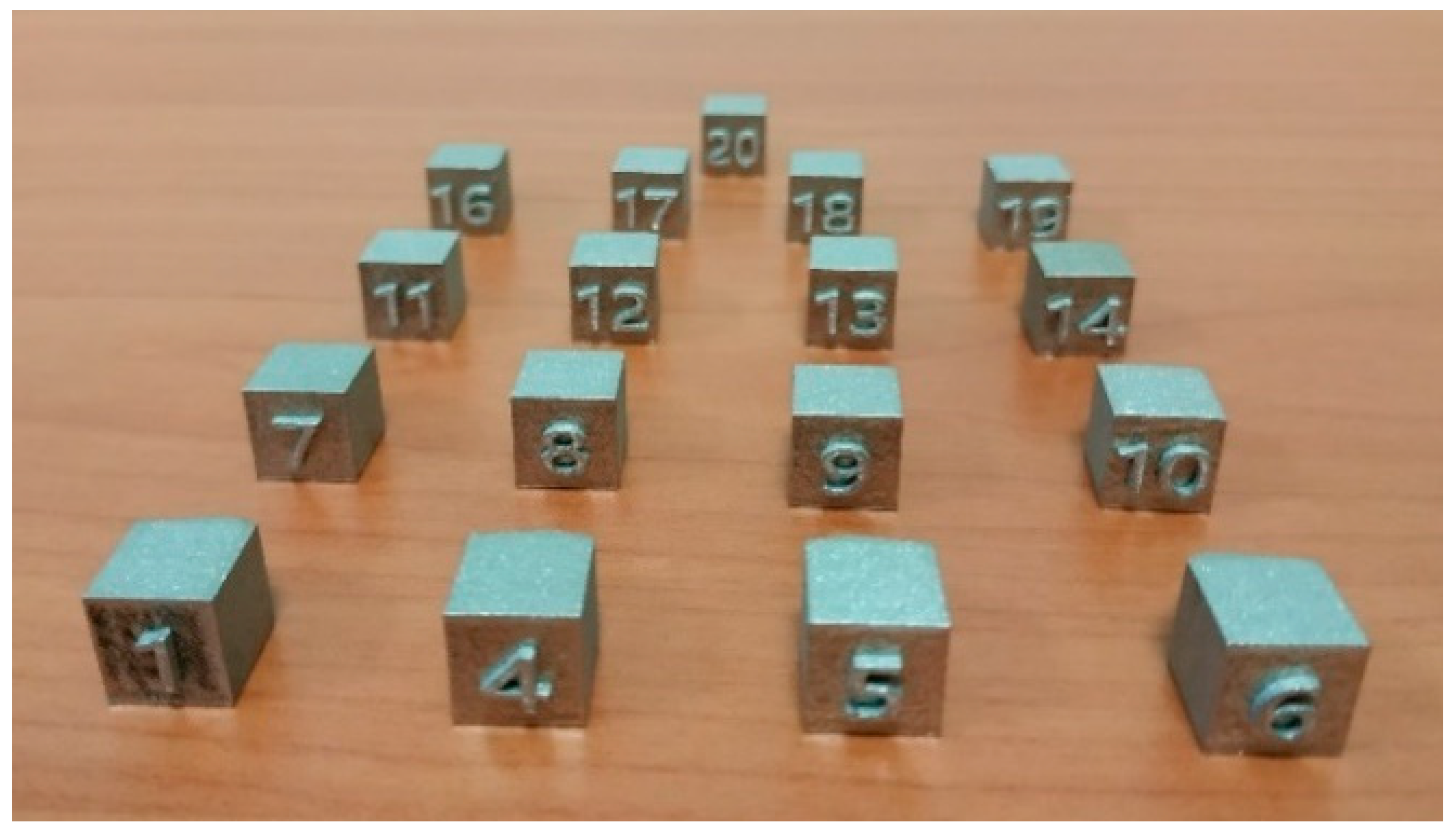
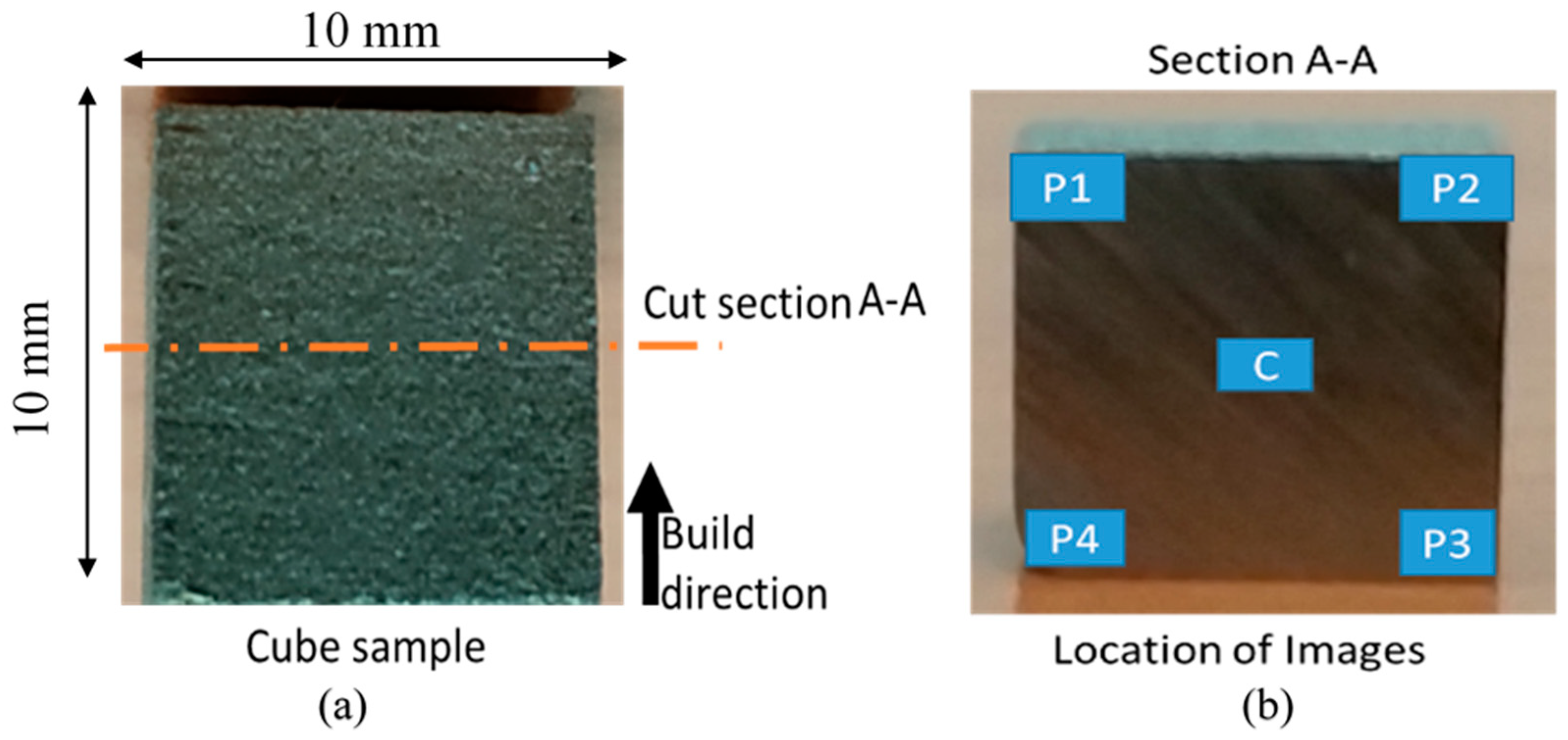
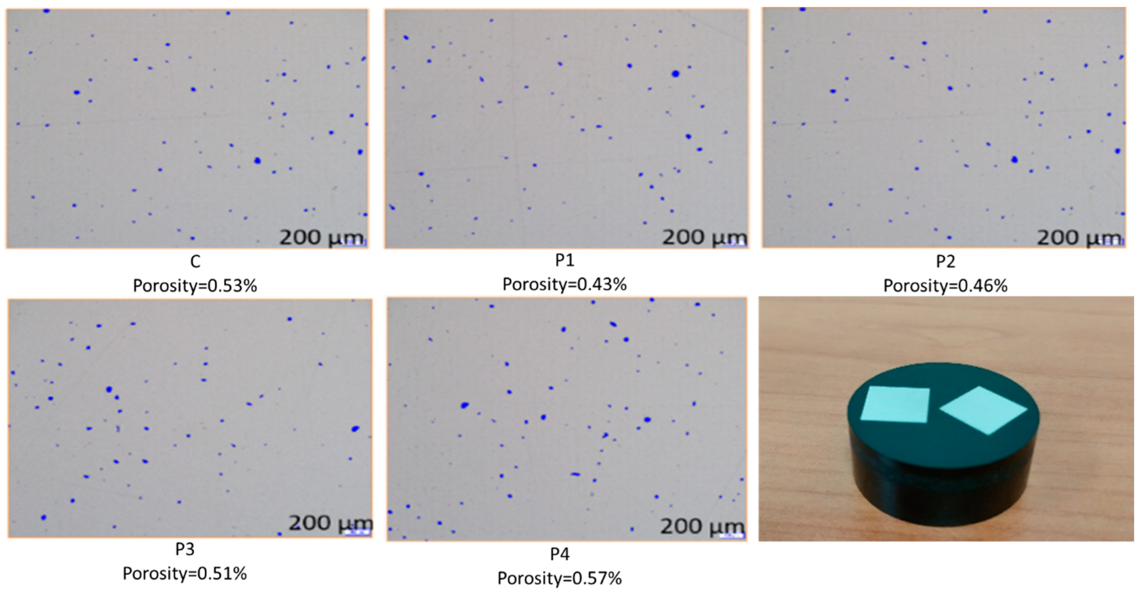
2.3. Experimental Procedure and Density Measurement

Specimens were built using an EOS M400-4 AM machine [36]. The machine has a total build volume of 400 × 400 × 400 mm and four 400 W fiber lasers that each work over an area of 250 × 250 mm, with a 50 mm overlap.
Cubic specimens with an edge length of 10 mm were fabricated using different laser powers, scan speeds, and hatch distances, with a constant layer thickness of 0.04 mm. The base powder material was SS316L by EOS, having a powder particle size distribution between 20 to 65 μm and typical chemical composition in weight percent as: Cr 18%, Ni 14%, Mo 2.5% and C 0.03%. Table 2 gives selected values of the parameters used and the measured relative densities. The parameter values are based on the usual ranges of AM machines, and in particular for EOS M400 machine when printing with SS316L powders. The printed SS316L samples are shown in Figure 1.
Then, the samples were cut, grinded and polished across their mid-section to measure the porosity, as shown in Figure 2a. An optical microscope was used capture the images and the positions on the cross section where images were captured are also displayed in Figure 2b.
Following that, the samples were etched and polished for optical imaging, and the optical images were analyzed using Avizo imaging software to investigate the porosity content, as illustrated in Figure 3. Finally, the average relative density was determined from the porosity area measurements through the Avizo software, and the results for all the fabricated specimens are given in Table 2.

3. Applied Regression Models and Modelling

This section describes three regression models used in this study. Table 3 provides the list of symbols used in the models.

3.1. Ridge Regression (RR)

The least squares regression is the most fundamental regression model. Linear regression is the simplest form of the least squares method, where the relationship between the variables is described by a line, which in matrix form can be expressed as
y = X β + ϵ
where y N is the dependent variable vector and X N × d is the data matrix representing d 1 independent variables and N rows, β is the coefficient vector, and ϵ   N is the random error vector [37]. The solution to the minimization of the sum of squared errors (SSE) with regard to β in Equation (2) is given by Equation (3):
S S E = ( y X β ) T ( y X β )
β ^ = ( X T X ) 1 X T y
RR is an estimation method that can be used to improve prediction in regression situations involving strongly correlated parameters. This approach can prevent incorrect regression coefficients induced by multicollinearity in the least squares regression [38]. As a result, RR is frequently employed to avoid overfitting by adding a regularization parameter λ 0   to the SSE function, as presented in Equation (4).
S S E = f ( β ) = 1 2 ( y X β ) T ( y X β ) + λ 2 | | β T β | | 2
The solution to Equation (4) is given by
β ^ = ( X T X + λ I d ) 1 X T y
where I is the d × d identity matrix. Equation (5) shows that if λ = 0 , the RR reduces to the linear regression. Compared to ordinary unbiased linear regression, RR decreases the complexity of the model and mitigates multicollinearity by accepting a small amount of bias to reduce the variance and the MSE, thus helping to improve the prediction accuracy.

3.2. Kernel Ridge Regression (KRR)

KRR addresses nonlinearity in data by applying a mapping function ϕ ( . ) that maps the data into a higher-dimensional space. The kernel function uses dot products such that K = k ( x i , x j ) = ϕ ( x i ) ,   ϕ ( x j ) [39,40]. The most used kernels are the linear, polynomial, and radial basis function kernels. For this study, the radial basis function kernel is used for both SVR and KRR and can be written as:
k ( x i ,   x j ) = e γ x i x j 2 = e 1 2 σ 2 | | x i x j | | 2
where γ = 1 2 σ 2 is a tuning parameter that represents the width of the radial basis function.
The vector β in Equation (1) can be expressed as a linear combination of the data points such that β = X T α . Rewriting the model in Equation (1) results in
y = X X T α + ϵ = G α + ϵ
where the matrix G = X X T is a Gram matrix.
When the kernel K replaces the Gramian matrix G in Equation (7), the KRR model becomes
y = K α + ϵ
The KRR function to be minimized with regard to the dual variable α becomes
f ( α ) = 1 2 ( y K α ) T ( y K α ) + λ 2 | | α | | 2
to which the solution is
α = ( K + λ I N ) 1 y
If the matrix ( K + λ I N ) is dense, the computational time has a complexity of O ( N 3 ) . Hence, iterative methods are the most suitable to compute α . Thus, the model in Equation (10) can be rewritten as
y = ( K + λ I N ) α
which is a linear system of equations and can be solved using iterative methods. Maalouf and Homouz [40] have applied the linear conjugate gradient to the Newton step, creating a truncated regularized kernel ridge regression (TR-KRR) algorithm. The TR-KRR algorithm is much faster than SVR without compromising accuracy. In this research, the KRR method is implemented as TR-KRR. Details about the TR-KRR algorithm can be found in [40].

3.3. Support Vector Regression (SVR)

SVM is a promising statistical learning technique based on the principle of structural risk minimization. This ML method is less sensitive to the dimensionality of the input and is more likely to achieve a lower generalization error of the regression model [2]. SVM is well known in classification problems. It is also applied to regression problems, in which case it is referred to as SVR. In brief, SVR finds an appropriate hyperplane to fit the data and provides flexibility in defining how much error is acceptable in the model.
The regression hyperplane is determined by maximizing the distances between nearby data points, known as support vectors, in a non-parametric regression model. The nonlinear SVR formulation is obtained by considering kernel functions employed to map inputs into high-dimensional feature spaces [41]. The goal of SVR is to search for a fitting function f ( x ) = { w ,   x } + b , where w is the weight vector, and b is the constant (bias), which has a deviation of less than a small value ε from the target ( y i ) acquired for the related training data set ( x i ) [16].
The objective function and constraints of SVR are given in Equations (12) and (13), respectively, as follows [42]:
Minimize :     1 2 w 2 + C   i = 1 n ( ξ i + ξ i * )
s .   t   { y i f ( x i ) ε + ξ i f ( x i ) y i ε + ξ i ξ i , ξ i * 0 ,   i = 1 , 2 , , n
where, ξ i and ξ i * are slack variables, and C is a regularization parameter that adds a penalty for each misclassified data point.
SVR simultaneously minimizes both the coefficient sizes and the prediction errors. The error term is included in the constraints, where the error is set as less than or equal to a specified margin, called the maximum error, ε [12]. The maximum error, ε , has to be properly tuned to obtain the desired accuracy of the model. Further, with the introduction of the Lagrange multipliers α and α * , and the application of the radial basis kernel function to the dot product of the input vectors, the following formula can be obtained:
f ( x ) = i = 1 n ( α i α i * ) k ( x i ,   x j ) + b
The radial base function kernel is introduced in Equation (6). The parameters ε and γ of the SVR model are user-defined.

3.4. Data Preparation and Model Evaluation

3.4.1. Data Pre-Processing

The quality of the data is a significant factor in the prediction process. Since multiple data sources were combined into one dataset, data cleansing, including data validation, outliers removal, and preparation for further analysis, should be completed before use [43]. The data cleansing process also modifies the data so that it is best suited to the data analysis task. The cleansing of the dataset highly affects the overall performance and robustness of the prediction model [44].
For this work, the initial data from the literature contained 232 observations. The cleansing process started with detecting potential outliers by observing the standardized residuals of the least squares regression. An observation with a standardized residual larger than 3 (absolute value) is deemed an outlier [45]. After the outlier removal process, 181 observations from the literature remained in the dataset. These observations from the literature were combined with the experimental results from the 20 specimens fabricated in the current work. Thus, the compiled dataset consisted of 201 observations ready to use for data analysis and modeling. The size of the dataset constructed in this study is almost double that presented in [22] (i.e., 112 points), implying the robustness of this study.
A clean, standardized, or normalized dataset is usually required before data analysis. This step is especially crucial when the data contains different parameter scales. For example, the layer thickness values in our dataset range from 0.02 mm to 0.25 mm, while the laser power values start at 30 W and increase to 400 W. These ranges in parameter values have to be scaled to a mean of zero and a standard deviation of one. Normalizing the dataset gives the input parameters an equal range of values, thus reducing their bias [46].

3.4.2. Model Evaluation with 10-Fold Cross-Validation

Cross-validation, which divides the dataset into several groups, is typically used to improve the estimate of the test error of a predictive model. It is a common approach since it is simple to understand and results in a less biased or positive judgment of the prediction ability of the model than other approaches [47].
In this study, 10-fold cross-validation is used to validate the models and provide better generalization. This technique randomly splits the dataset into k groups (usually k = 5 or 10) or folds of roughly equal size. The initial fold contains the test data that are used for testing the generalization ability of the model, while the remaining k − 1 folds contain the training and validation data used for formulating the model [47]. The accuracy of each model is evaluated using the average of the MSEs and the R2 values from the 10-fold cross-validation. All the regression models have been developed and tested using MATLAB R 2021a.

4. Results and Discussion

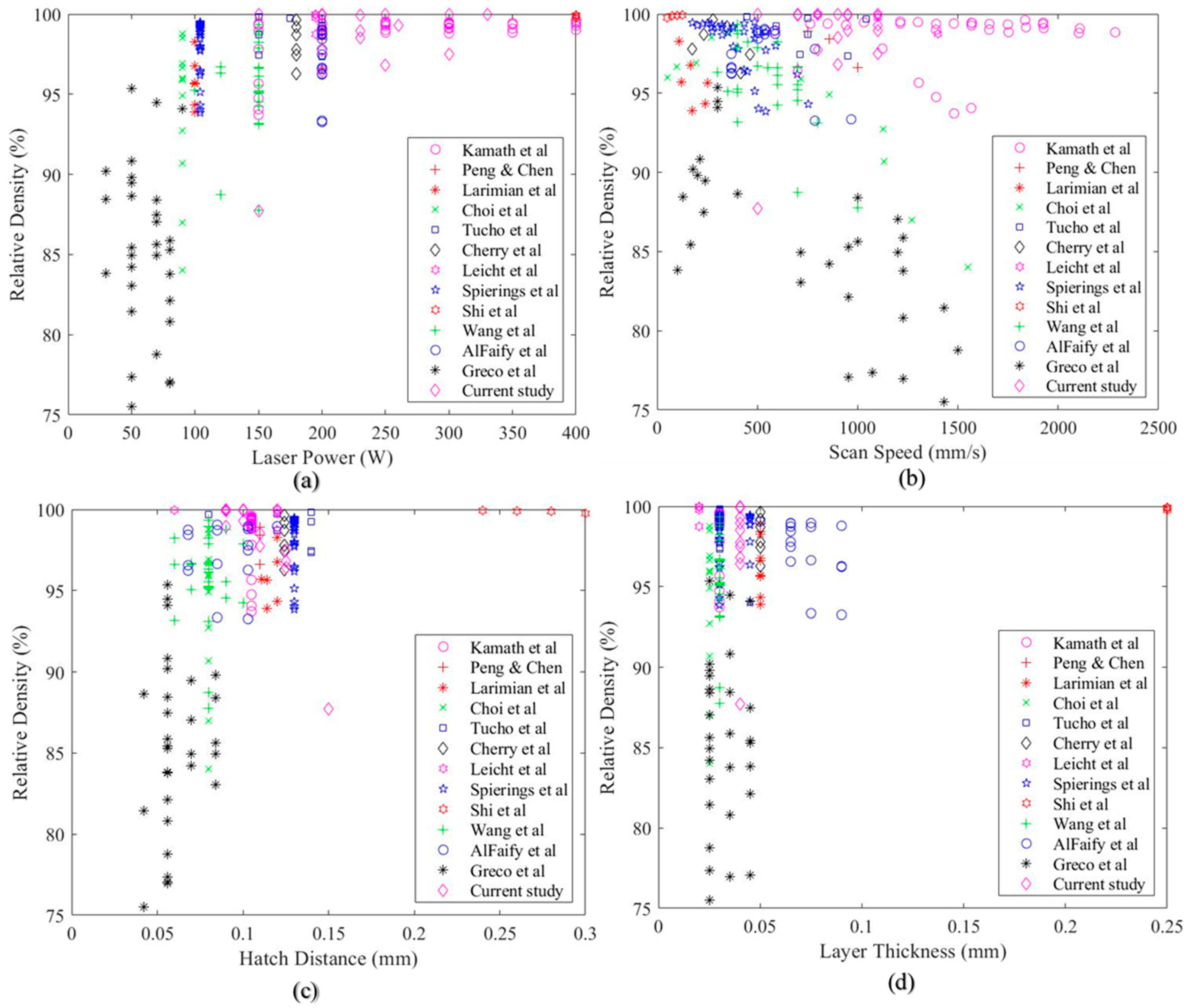
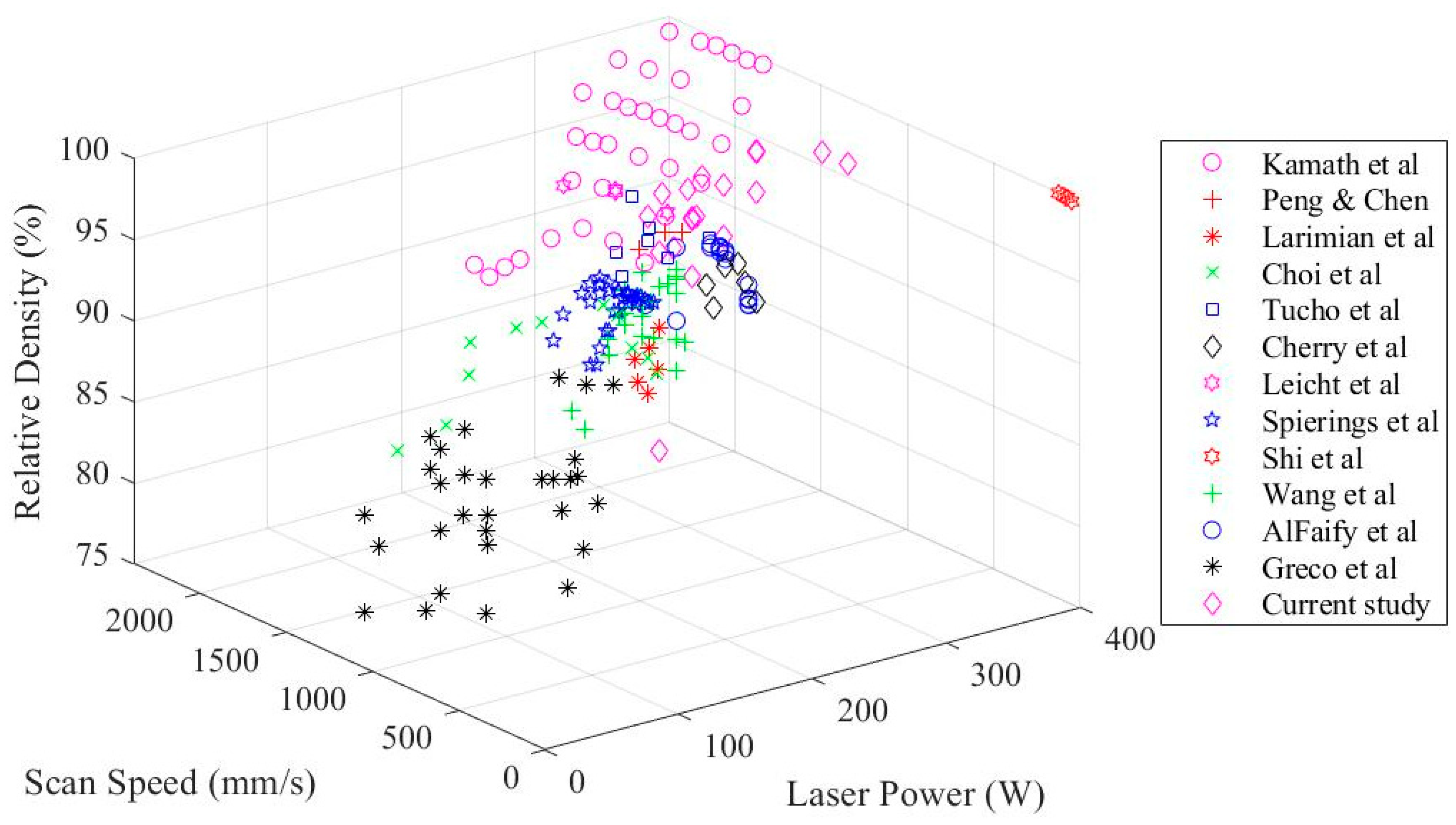
4.1. Analysis of Data Plots

The properties of the SLM-manufactured parts depend strongly on the input process parameters. Thus, it is crucial to understand the relationships between the main process parameters and the fabricated part characteristics. Although the compiled dataset is a subset of the experimental data available on the relative density of SS316L parts fabricated by SLM, it may provide valuable insight into the relationships between the process parameters and the measured relative density within the investigated range of parameters.
Figure 4 shows the relative density versus the laser power, scan speed, hatch distance, and layer thickness of the literature data combined with our experimental results. The variation in the process parameters results in the variation in the relative density. The process parameters in the compiled dataset have the following ranges: laser power between 30 and 400 W, scanning speed between 50 and 2400 mm/s, hatch distance between 0.04 and 0.3 mm, and layer thickness between 0.02 and 0.25 mm. The relative density of the samples ranges from 75% to 100%.
Figure 4a shows that the relative density is greater than 90% when the laser power is above 150 W. As the laser power and thermal energy from the laser beam increase, a greater percentage of the material within the volume is heated, possibly above its melting point. As a result, less material is left intact or partially melted, resulting in a higher relative density [22]. In contrast, low laser power may result in insufficient melting of the powder, as well as a reduced depth of the laser penetration into the powder layer, which is insufficient to melt the powder fully and fuse the layers [48]. Thus, increasing the laser power may improve and enhance the relative density of the parts.
Furthermore, in Figure 4b, a high relative density is observed when the scan speed exceeds 1500 mm/s. However, below a scan speed of 1500 mm/s, there is no clear correlation between the scan speed and relative density based on this dataset. The lower scan speed may incur irregular molten pools, which may yield larger grains and pores. Yusuf et al. [49] have reported that a lower scan speed increased laser penetration depth, and inhomogeneous rapid solidification occurred, resulting in lower relative density. A study in [30] has also noted that samples processed at higher scan speeds had better densification and more refined microstructure than samples processed at lower scan speeds.
Concerning the hatch distance, as shown in Figure 4c, most of the experiments used small hatch distances in the range of 0.05–0.15 mm. Small hatch distances ensure overlapping melt pools and hence, less pore formation than larger hatch distances that result in weak overlapping and provide good conditions for pore formation [31].
Figure 4d shows the experimental results of different layer thicknesses and the resulting measured relative density of the parts. While there is no clear correlation between the relative density and layer thickness in the range of 0.025–0.05 mm, increasing the layer thickness from 0.05 mm to 0.1 mm results in a higher relative density. The appropriate layer thickness adjustment allows the laser spots to overlap and result in sufficient melting of the powder. However, if the powder layer is too thick, it would be hard to create a melt pool with enough depth to melt and fuse the layers [48].
Based on Figure 4a,b, scan speed greater than 1500 mm/s and laser powers greater than 150 W achieve high relative density. Figure 5 illustrates the combined effects of the laser power and scan speed on the relative density. High laser power appears to compensate for high scanning speed, preventing leftover unmelted powder. When the laser power increases, the same volume of powder must absorb the same amount of thermal energy to melt in a shorter time interval [28]. Based on the observation in Figure 4 and Figure 5, the relative density of SS316L parts is strongly dependent on the process parameters. Setting the process parameters appropriately will yield fabricated parts with high relative density.

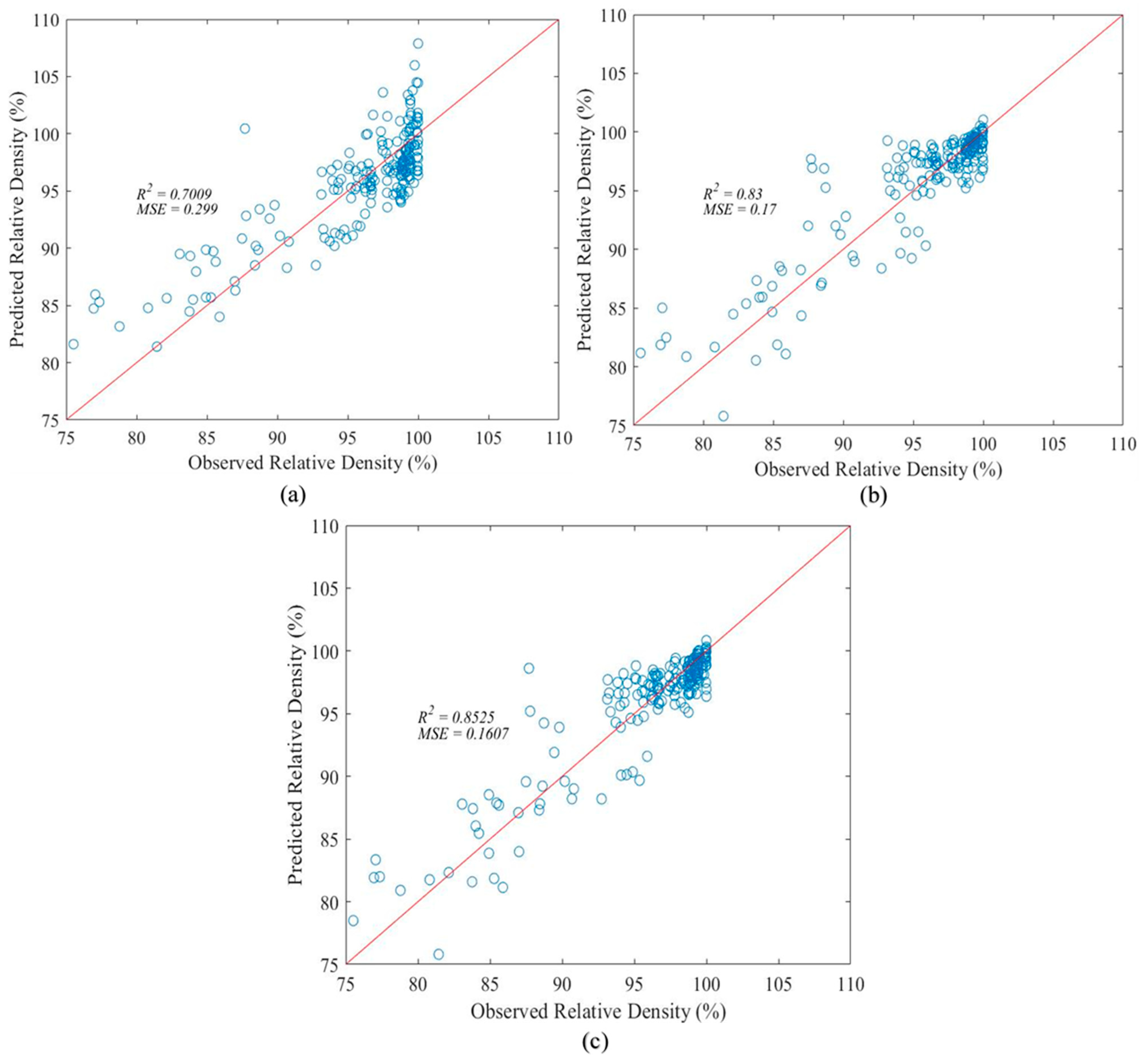
4.2. Analysis of Regression Results

To check the ability and adequacy of the established models related to the real SLM system, Figure 6 compares the relative density data determined experimentally with the values predicted using (a) RR, (b) SVR, and (c) KRR. Ideally, if the predicted values are equal to the actual data, the points should lie closer to the diagonal line on the graph.
The RR model results presented in Figure 6a show the lowest accuracy compared to the other models. Furthermore, the plot of the SVR presented in Figure 6b shows better agreement between the predicted and actual values, indicating a higher accuracy. Finally, Figure 6c demonstrates the predicted vs. actual plot of the KRR model. This model gives the highest accuracy, as the values were distributed closer to the diagonal line than other models. The KRR model may be adequate for predicting the relative density and strong enough to be used in future applications.
Table 4 presents the optimal tuning parameters for each model and their corresponding accuracy represented by the R2 and MSE. An R2 of 0.701 and an MSE of 0.299 were obtained using RR with a tuning parameter (λ) of 0.006. Moreover, SVR showed a better performance with R2 of 0.83 and MSE of 0.17, along with tuning parameters γ and ε equal to 0.4 and 0.05, respectively. Finally, the KRR resulted in the best accuracy among the three models with an R2 of 0.853 and MSE of 0.1607, with tuning parameters λ and σ equal to 0.01 and 2.9, respectively. KRR has shown the best performance as it captures the nonlinearities and complex interactions of the SLM process. It may be good to note that the studied machine learning methods have employed a grid search approach to find the optimal tunning parameters. However, there is still room to find the optimal tunning parameters effectively.
KRR was not used in Barrionuevo et al. (2021), and SVM was one of the best regression algorithms in their study. This implies that KRR may have better prediction capability for the relative density of the SS316L parts than other regression techniques. The present paper complements the recent study in [16] with the doubled data size and consideration of an additional better regression algorithm (i.e., KRR).

5. Conclusions

The relative density of SS316L fabricated by SLM has been studied using data from the literature merged with experimental data collected for this study. Different plots visualize the trends between the input process parameters (i.e., laser power, scan speed, hatch distance, and layer thickness) and the corresponding relative density. ML techniques, such as RR, SVR, and KRR, are used to predict the relative density of the parts, and their performances are compared.
Based on observational analysis of the dataset, the laser power and scan speed have a strong effect on the relative density: high power and high speed would generate better densification of the parts. In comparisons between the RR, SVR, and KRR models, KRR outperformed RR and showed a slightly better performance than SVR based on its lower MSE and higher R2 values. The KRR may have sufficient predictability for the relative density of the SS316L parts as a function of the laser power, scan speed, hatch distance, and layer thickness.
The methods and findings in this study would be beneficial for AM designers who seek high-precision models to predict AM part properties using input process parameters. It could also reduce the expense of more experimental trials by prescribing the optimal process parameters, consuming less energy, and generating environmental benefits [50]. The presented machine learning methods predict the porosity of 3D printed materials by identifying the relationship between the process parameters and pores. Thus, the formation of pores can be inhibited by finding the appropriate process parameters. Future work can use the developed predictive models combined with an optimization method to prescribe the optimal process parameters for minimizing pores.

Author Contributions

Conceptualization, I.B. and H.A. (Heungjo An); Data curation, H.A. (Hind Abdulla), I.B. and H.A. (Heungjo An); Formal analysis, H.A. (Hind Abdulla), M.M. and I.B.; Funding acquisition, I.B. and H.A. (Heungjo An); Methodology, I.B. and M.M.; Project administration, I.B. and H.A. (Heungjo An); Software, H.A. (Hind Abdulla) and M.M.; Writing—original draft, H.A. (Hind Abdulla); Writing—review & editing, M.M., I.B. and H.A. (Heungjo An). All authors have read and agreed to the published version of the manuscript.

Funding

This research was funded by Khalifa University of Science and Technology grant number RCII-2019-003.

Institutional Review Board Statement

Not applicable.

Informed Consent Statement

Not applicable.

Data Availability Statement

Not applicable.

Conflicts of Interest

The authors declare no conflict of interest.

References

  1. ISO/ASTM. ASTM Standard 52900; Additive Manufacturing—General Principles Terminology. ISO: Geneva, Switzerland, 2015. [Google Scholar]
  2. Baturynska, I.; Martinsen, K. Prediction of Geometry Deviations in Additive Manufactured Parts: Comparison of Linear Regression with Machine Learning Algorithms. J. Intell. Manuf. 2021, 32, 179–200. [Google Scholar] [CrossRef]
  3. Peng, T.; Chen, C. Influence of Energy Density on Energy Demand and Porosity of 316L Stainless Steel Fabricated by Selective Laser Melting. Int. J. Precis. Eng. Manuf. Green Technol. 2018, 5, 55–62. [Google Scholar] [CrossRef]
  4. Garg, A.; Tai, K.; Lee, C.H.; Savalani, M.M. A Hybrid M5′-Genetic Programming Approach for Ensuring Greater Trustworthiness of Prediction Ability in Modelling of FDM Process. J. Intell. Manuf. 2014, 25, 1349–1365. [Google Scholar] [CrossRef]
  5. Garg, A.; Tai, K.; Savalani, M.M. State-of-the-Art in Empirical Modelling of Rapid Prototyping Processes. Rapid Prototyp. J. 2014, 20, 164–178. [Google Scholar] [CrossRef]
  6. Mahamood, R.M.; Akinlabi, E.T. Processing Parameters Optimization for Material Deposition Efficiency in Laser Metal Deposited Titanium Alloy. Lasers Manuf. Mater. Process. 2016, 3, 9–21. [Google Scholar] [CrossRef]
  7. Averyanova, M.; Cicala, E.; Bertrand, P.; Grevey, D. Experimental Design Approach to Optimize Selective Laser Melting of Martensitic 17-4 PH Powder: Part I—Single Laser Tracks and First Layer. Rapid Prototyp. J. 2012, 18, 28–37. [Google Scholar] [CrossRef]
  8. Srivastava, M.; Maheshwari, S.; Kundra, T.; Rathee, S. Multi-Response Optimization of Fused Deposition Modelling Process Parameters of ABS Using Response Surface Methodology (RSM)-Based Desirability Analysis. Mater. Today Proc. 2017, 4, 1972–1977. [Google Scholar] [CrossRef]
  9. Wang, C.; Tan, X.P.; Tor, S.B.; Lim, C.S. Machine Learning in Additive Manufacturing: State-of-the-Art and Perspectives. Addit. Manuf. 2020, 36, 101538. [Google Scholar] [CrossRef]
  10. Miranda, G.; Faria, S.; Bartolomeu, F.; Pinto, E.; Madeira, S.; Mateus, A.; Carreira, P.; Alves, N.; Silva, F.S.; Carvalho, O. Predictive Models for Physical and Mechanical Properties of 316L Stainless Steel Produced by Selective Laser Melting. Mater. Sci. Eng. A 2016, 657, 43–56. [Google Scholar] [CrossRef]
  11. Asilturk, I.; Kahramanli, H.; El Mounayri, H. Prediction of Cutting Forces and Surface Roughness Using Artificial Neural Network (ANN) and Support Vector Regression (SVR) in Turning 4140 Steel. Mater. Sci. Technol. 2013, 28, 980–986. [Google Scholar] [CrossRef]
  12. Desu, R.K.; Guntuku, S.C.; Aditya, B.; Gupta, A.K. Support Vector Regression Based Flow Stress Prediction in Austenitic Stainless Steel 304. Procedia Mater. Sci. 2014, 6, 368–375. [Google Scholar] [CrossRef] [Green Version]
  13. Owolabi, T.O.; Akande, K.O.; Olatunji, S.O. Estimation of Superconducting Transition Temperature TC for Superconductors of the Doped MgB2 System from the Crystal Lattice Parameters Using Support Vector Regression. J. Supercond. Nov. Magn. 2015, 28, 75–81. [Google Scholar] [CrossRef]
  14. Pham, T.L.; Nguyen, N.D.; Nguyen, V.D.; Kino, H.; Miyake, T.; Dam, H.C. Learning Structure-Property Relationship in Crystalline Materials: A Study of Lanthanide–Transition Metal Alloys. J. Chem. Phys. 2018, 148, 204106. [Google Scholar] [CrossRef] [PubMed]
  15. Kauwe, S.K.; Rhone, T.D.; Sparks, T.D. Data-Driven Studies of Li-Ion-Battery Materials. Crystals 2019, 9, 54. [Google Scholar] [CrossRef] [Green Version]
  16. Wen, C.; Zhang, Y.; Wang, C.; Xue, D.; Bai, Y.; Antonov, S.; Dai, L.; Lookman, T.; Su, Y. Machine Learning Assisted Design of High Entropy Alloys with Desired Property. Acta Mater. 2019, 170, 109–117. [Google Scholar] [CrossRef] [Green Version]
  17. Goh, G.D.; Sing, S.L.; Yeong, W.Y. A Review on Machine Learning in 3D Printing: Applications, Potential, and Challenges. Artif. Intell. Rev. 2021, 54, 63–94. [Google Scholar] [CrossRef]
  18. Liu, Y.; Kang, M.; Wu, Y.; Wang, M.; Gao, H. Machine Learning to Optimize Additive Manufacturing Parameters for Laser Powder Bed Fusion of Inconel 718. In Proceedings of the 9th International Symposium on Superalloy 718 & Derivatives: Energy, Aerospace, and Industrial Applications; No. 800; Springer: Cham, Switzerland, 2018; pp. 389–404. [Google Scholar] [CrossRef]
  19. Singh, A.; Cooper, D.E.; Blundell, N.J.; Gibbons, G.J.; Pratihar, D.K. Modelling of Direct Metal Laser Sintering of EOS DM20 Bronze Using Neural Networks and Genetic Algorithms. In Proceedings of the 37th International Matador 2012 Conference;International Matador Conference; Springer: London, UK, 2013; pp. 395–398. [Google Scholar]
  20. Tapia, G.; Elwany, A.H.; Sang, H. Prediction of Porosity in Metal-Based Additive Manufacturing Using Spatial Gaussian Process Models. Addit. Manuf. 2016, 12 Pt B, 282–290. [Google Scholar] [CrossRef]
  21. Imani, F.; Gaikwad, A.; Montazeri, M.; Rao, P.; Yang, H.; Reutzel, E. Layerwise In-Process Quality Monitoring in Laser Powder Bed Fusion. In Proceedings of the ASME 2018 13th International Manufacturing Science and Engineering Conference, College Station, TX, USA, 18–22 June 2018; American Society of Mechanical Engineers: New York, NY, USA, 2018; Volume 1, pp. 1–14. [Google Scholar] [CrossRef]
  22. Barrionuevo, G.O.; Ramos-Grez, J.A.; Walczak, M.; Betancourt, C.A. Comparative Evaluation of Supervised Machine Learning Algorithms in the Prediction of the Relative Density of 316L Stainless Steel Fabricated by Selective Laser Melting. Int. J. Adv. Manuf. Technol. 2021, 113, 419–433. [Google Scholar] [CrossRef]
  23. Lee, S.; Peng, J.; Shin, D.; Choi, Y.S. Data Analytics Approach for Melt-Pool Geometries in Metal Additive Manufacturing. Sci. Technol. Adv. Mater. 2019, 20, 972–978. [Google Scholar] [CrossRef] [Green Version]
  24. Wang, C.; Tan, X.; Liu, E.; Tor, S.B. Process Parameter Optimization and Mechanical Properties for Additively Manufactured Stainless Steel 316L Parts by Selective Electron Beam Melting. Mater. Des. 2018, 147, 157–166. [Google Scholar] [CrossRef]
  25. Kamath, C.; El-Dasher, B.; Gallegos, G.F.; King, W.E.; Sisto, A. Density of Additively-Manufactured, 316L SS Parts Using Laser Powder-Bed Fusion at Powers up to 400 W. Int. J. Adv. Manuf. Technol. 2014, 74, 65–78. [Google Scholar] [CrossRef] [Green Version]
  26. Spierings, A.B.; Herres, N.; Levy, G. Influence of the Particle Size Distribution on Surface Quality and Mechanical Properties in AM Steel Parts. Rapid Prototyp. J. 2020, 17. [Google Scholar] [CrossRef] [Green Version]
  27. Choi, J.P.; Shin, G.H.; Brochu, M.; Kim, Y.J.; Yang, S.S.; Kim, K.T.; Yang, D.Y.; Lee, C.W.; Yu, J.H. Densification Behavior of 316L Stainless Steel Parts Fabricated by Selective Laser Melting by Variation in Laser Energy Density. Mater. Trans. 2016, 57, 1952–1959. [Google Scholar] [CrossRef] [Green Version]
  28. Greco, S.; Gutzeit, K.; Hotz, H.; Kirsch, B.; Aurich, J.C. Selective Laser Melting (SLM) of AISI 316L—Impact of Laser Power, Layer Thickness, and Hatch Spacing on Roughness, Density, and Microhardness at Constant Input Energy Density. Int. J. Adv. Manuf. Technol. 2020, 108, 1551–1562. [Google Scholar] [CrossRef]
  29. Leicht, A.; Rashidi, M.; Klement, U.; Hryha, E. Effect of Process Parameters on the Microstructure, Tensile Strength and Productivity of 316L Parts Produced by Laser Powder Bed Fusion. Mater. Charact. 2020, 159, 110016. [Google Scholar] [CrossRef]
  30. Larimian, T.; Kannan, M.; Grzesiak, D.; AlMangour, B.; Borkar, T. Effect of Energy Density and Scanning Strategy on Densification, Microstructure and Mechanical Properties of 316L Stainless Steel Processed via Selective Laser Melting. Mater. Sci. Eng. A 2020, 770, 138455. [Google Scholar] [CrossRef]
  31. Tucho, W.M.; Lysne, V.H.; Austbø, H.; Sjolyst-Kverneland, A.; Hansen, V. Investigation of Effects of Process Parameters on Microstructure and Hardness of SLM Manufactured SS316L. J. Alloys Compd. 2018, 740, 910–925. [Google Scholar] [CrossRef]
  32. Cherry, J.A.; Davies, H.M.; Mehmood, S.; Lavery, N.P.; Brown, S.G.R.; Sienz, J. Investigation into the Effect of Process Parameters on Microstructural and Physical Properties of 316L Stainless Steel Parts by Selective Laser Melting. Int. J. Adv. Manuf. Technol. 2014, 76, 869–879. [Google Scholar] [CrossRef] [Green Version]
  33. AlFaify, A.; Hughes, J.; Ridgway, K. Controlling the Porosity of 316L Stainless Steel Parts Manufactured via the Powder Bed Fusion Process. Rapid Prototyp. J. 2019, 25, 162–175. [Google Scholar] [CrossRef]
  34. Shi, W.; Wang, P.; Liu, Y.; Hou, Y.; Han, G. Properties of 316L Formed by a 400 W Power Laser Selective Laser Melting with 250 μm Layer Thickness. Powder Technol. 2020, 360, 151–164. [Google Scholar] [CrossRef]
  35. Wang, D.; Liu, Y.; Yang, Y.; Xiao, D. Theoretical and Experimental Study on Surface Roughness of 316L Stainless Steel Metal Parts Obtained through Selective Laser Melting. Rapid Prototyp. J. 2016, 22, 706–716. [Google Scholar] [CrossRef]
  36. EOS GmbH. Large and Ultra-Fast 3D Printer with 4 Laser. Available online: https://www.eos.info/en/additive-manufacturing/3d-printing-metal/eos-metal-systems/eos-m-400-4 (accessed on 15 September 2021).
  37. Montgomery, D.C.; Peck, E.A.; Vining, G.G. Introduction to Linear Regression Analysis, 5th ed.; John Wiley & Sons: Hoboken, NJ, USA, 2012. [Google Scholar]
  38. Salim, I.; Hamza, A.B. Ridge Regression Neural Network for Pediatric Bone Age Assessment. Multimed. Tools Appl. 2021, 80, 30461–30478. [Google Scholar] [CrossRef]
  39. Schölkopf, B.; Vovk, V.; Luo, Z. ‘Kernel Ridge Regression’, in Empirical Inference; Springer: Berlin/Heidelberg, Germany, 2013. [Google Scholar] [CrossRef]
  40. Maalouf, M.; Homouz, D. Kernel Ridge Regression Using Truncated Newton Method. Knowledge-Based Syst. 2014, 71, 339–344. [Google Scholar] [CrossRef]
  41. Goswami, K.; Samuel, G.L. Support Vector Machine Regression for Predicting Dimensional Features of Die-Sinking Electrical Discharge Machined Components. Procedia CIRP 2021, 99, 508–513. [Google Scholar] [CrossRef]
  42. Zhao, Y.; Jiang, M.; Lu, X. Support Vector Machine Regression Based Supercapacitor’s Dynamic Characteristics Model. In Proceedings of the 2017 International Conference on Consumer Electronics and Devices (ICCED), London, UK, 14–17 July 2017; pp. 27–30. [Google Scholar] [CrossRef]
  43. Loshin, D. The Practitioner’s Guide to Data Quality Improvement; Loshin, D., Ed.; Elsevier: Amsterdam, The Netherlands, 2011. [Google Scholar]
  44. Tidemann, A.; Høverstad, B.A.; Langseth, H.; Öztürk, P. Effects of Scale on Load Prediction Algorithms. IET Conf. Publ. 2013, 2013, 615. [Google Scholar] [CrossRef] [Green Version]
  45. Raj, S.; Kannan, S. Detection of Outliers in Regression Model for Medical Data. Int. J. Med. Res. Health Sci. 2017, 6, 50–56. [Google Scholar]
  46. Maalouf, M.; Barsoum, Z. Failure Strength Prediction of Aluminum Spot-Welded Joints Using Kernel Ridge Regression. Int. J. Adv. Manuf. Technol. 2017, 91, 3717–3725. [Google Scholar] [CrossRef]
  47. de Rooij, M.; Weeda, W. Cross-Validation: A Method Every Psychologist Should Know. Adv. Methods Pract. Psychol. Sci. 2020, 3, 248–263. [Google Scholar] [CrossRef]
  48. Brown, C.U.; Jacob, G.; Possolo, A.; Beauchamp, C.; Peltz, M.; Stoudt, M.; Donmez, A. The Effects of Laser Powder Bed Fusion Process Parameters on Material Hardness and Density for Nickel Alloy 625. NIST Adv. Manuf. Ser. 2018, 2018, 100–119. [Google Scholar]
  49. Yusuf, S.M.; Chen, Y.; Boardman, R.; Yang, S.; Gao, N. Investigation on Porosity and Microhardness of 316L Stainless Steel Fabricated by Selective Laser Melting. Metals 2017, 7, 64. [Google Scholar] [CrossRef] [Green Version]
  50. An, H.; Byon, Y.J.; Cho, C.S. Economic and Environmental Evaluation of a Brick Delivery System Based on Multi-Trip Vehicle Loader Routing Problem for Small Construction Sites. Sustainability 2018, 10, 1427. [Google Scholar] [CrossRef] [Green Version]
Figure 1. SS316L cube samples fabricated using the EOS M400-4 AM machine.
Applsci 12 04252 g001
Figure 2. (a) Sample cube cross-sectioned for measurement of porosity (10 × 10 × 10 mm) (b) Locations of optical imaging on the cut surface adapted from [26].
Applsci 12 04252 g002
Figure 3. Optical images from Sample #3 using Avizo imaging software to measure porosity.
Applsci 12 04252 g003
Figure 4. Plots of the relative density against (a) laser power, (b) scan speed, (c) hatch distance, and (d) layer thickness.
Applsci 12 04252 g004
Figure 5. 3D plot of the relative density versus the laser power and scan speed.
Applsci 12 04252 g005
Figure 6. Predicted vs. actual relative density for (a) RR, (b) SVR, and (c) KRR using 10-fold cross-validation.
Applsci 12 04252 g006
Table 1. Summary of experimental conditions of studies used for data collection.
AuthorsExperimental Conditions
MachinePowderFabricated PartsDensity/Porosity Measurement Method
Kamath
et al. [25]
-
Concept Laser GmbH M2 machine under Argon atmosphere.
-
Processes performed at room temperature.
-
Machine has a 400-W fiber laser.
-
Two types of SS316L powders: CL20 ES and LPW.
Pillars of surface area 10 × 10 mm2.Archimedes method and scanning electron microscope.
Spierings
et al. [26]
-
Concept Laser GmbH M1 machine equipped with an Nd: YAG solid-state laser.
-
Maximum laser power of 105W.
-
Chessboard-like structure scan strategy.
-
Powder M and 16-45: Gaussian particle size distribution.
-
Powder 1.4404–CL20: Asymmetric distribution.
Cubes of size 5 × 5 × 5 mm2.Archimedes method.
Choi
et al. [27]
-
Concept Laser GmbH Mlab-Cusing under Argon atmosphere.
-
Machine equipped with Yb:YAG fiber laser, effective power of 100 W.
-
Line scanning strategy.
-
Processes performed at room temperature.
-
SS316L CL20ES powder.
-
Spherical morphology and irregularly shaped particles.
-
Narrow particle size distribution.
Cubes of size 10 × 10 × 10 mm3. Archimedes method.
Greco
et al. [28]
-
Concept Laser GmbH Mlab-Cusing equipped with Nd:YAG fiber laser.
-
Maximum power of 100 W.
-
Building volume is 90 × 90 × 80 mm3.
-
Maximum grain size of 50 μm.
Cubes of size 8 × 8 × 8 mm3.Relative density was determined from an analytical model describing the parts dimensions, mass, and density of the material used.
Leicht
et al. [29]
-
EOS GmbH M290 machine.
-
Ar environment and oxygen content below 0.1%.
-
Stripe scanning scan strategy.
-
Gas-atomized 316L powder.
-
Size distribution of 25–53 μm.
Rectangular prisms of 72 × 12 × 2.5 mm3.Light optical microscopy micrographs.
Larimian
et al. [30]
-
SLM Solutions GmbH under Argon atmosphere.
-
Equipped with fiber laser with a power of 100 W.
-
Automatic powder layering mechanism.
-
Gas-atomized 316L powder.
-
Different particle size distributions.
-
Horizontally built Blocks.
-
Rectangular prisms of 80 × 10 × 6 mm3.
Scanning electron microscope images using ImageJ software.
Tucho
et al. [31]
-
SLM Solutions GmbH 280HL machine under Argon atmosphere.
-
Equipped with 400 W fiber laser.
-Cubes of size 10 × 10 × 10 mm3.Scanning electron microscope images using ImageJ software.
Peng and Chen. [3]Renishaw AM250.-Cubes of size 10 × 10 × 10 mm3.Metallographic microscope (Leica DM2700P) after polishing the samples.
Cherry
et al. [32]
-
Renishaw AM250 equipped with Nd:YAG laser.
-
Maximum power of 200 W.
-
Ambient temperature was maintained at 21 °C.
-
Particle size range 15 to 45 μm manufactured via gas atomization.
Cubes of size 10 × 10 × 10 mm3.In-house image analysis software. Microstructural analysis using a JEOL-35C scanning electron microscope.
AlFaify
et al. [33]
-
Renishaw AM250.
-
Equipped with 200W pulsed laser.
-
Machine build volume of 250 × 250 × 300 mm3.
-
Particle size range 15–45 μm manufactured via gas atomization.
Cubes of size10 × 10 × 10 mm3.Archimedes method.
Shi
et al. [34]
-
Renishaw AM400 equipped with Nd: YAG laser.
-
Maximum power of 400 W.
-
Machine build volume of 250 × 250 × 300 mm3.
-
Meander scan strategy.
-
Particle size range 5–41 μm manufactured via gas atomization.
Specimen dimensions of 5 × 5 × 10 mm3.Optical microscope images using Image J.
Wang
et al. [35]
-
Laseradd DiMetal-100 machine
-
Maximum laser power 200 W.
-
Building envelope is 100 × 100 × 120 mm.
-
Process performed under argon or nitrogen atmosphere.
-
Gas-atomized 316L powder.
-
Average particle size of 17 μm.
-
Density of 4.04 g/cm3.
Cubes of size10 × 10 × 5 mm3.Relative density was measured through the drainage method.
Table 2. Selected process parameters and measured relative density for the produced samples.
Sample No.Power (W)Speed (mm/s)Hatch Distance (mm)Relative Density (%)
11505000.090100.00
21505000.10099.97
31505000.12587.70
42007000.090100.00
52007000.10099.95
62007000.12596.41
72509000.090100.00
82509000.10099.96
92509000.12596.80
1030011000.090100.00
1130011000.10099.98
1230011000.12597.50
132309500.09099.93
143308000.120100.00
153309500.090100.00
162008000.11097.72
172009500.09098.93
182309000.11098.51
1923011000.09098.93
20 26011000.10099.30
Table 3. List of symbols used in the models.
SymbolsRemarks
β Coefficient vector in RR and KRR
ϵ Random error vector in RR and KRR
λ Regularization parameter in RR and KRR
I d d × d identity matrix in RR and KRR
γ Tuning parameter in the KRR radial basis function ( = 1 2 σ 2 )
σ Tuning parameter in the KRR radial basis function
α Dual variable vector in KRR
ξ i , ξ i * Slack variables in SVR
C Regularization parameter that adds a penalty in SVR
ε Maximum error in SVR
α ,   α * Lagrange multipliers in SVR
Table 4. Optimal tuning parameters and accuracy of the models.
ModelOptimal ParametersAccuracy
R2MSE
RRλ = 0.0060.7010.299
SVRγ = 0.4, ε = 0.050.8300.170
KRRλ = 0.01, σ = 2.90.8530.161
Publisher’s Note: MDPI stays neutral with regard to jurisdictional claims in published maps and institutional affiliations.

