
Speed-Flow-Geometric Relationship for Urban Roads Network


 ,
, 
Abstract
:1. Introduction
2. Related Literatures Overview
2.1. Characteristics of Speed-Flow Relationship Models
2.2. Regression Analysis
3. Methodology
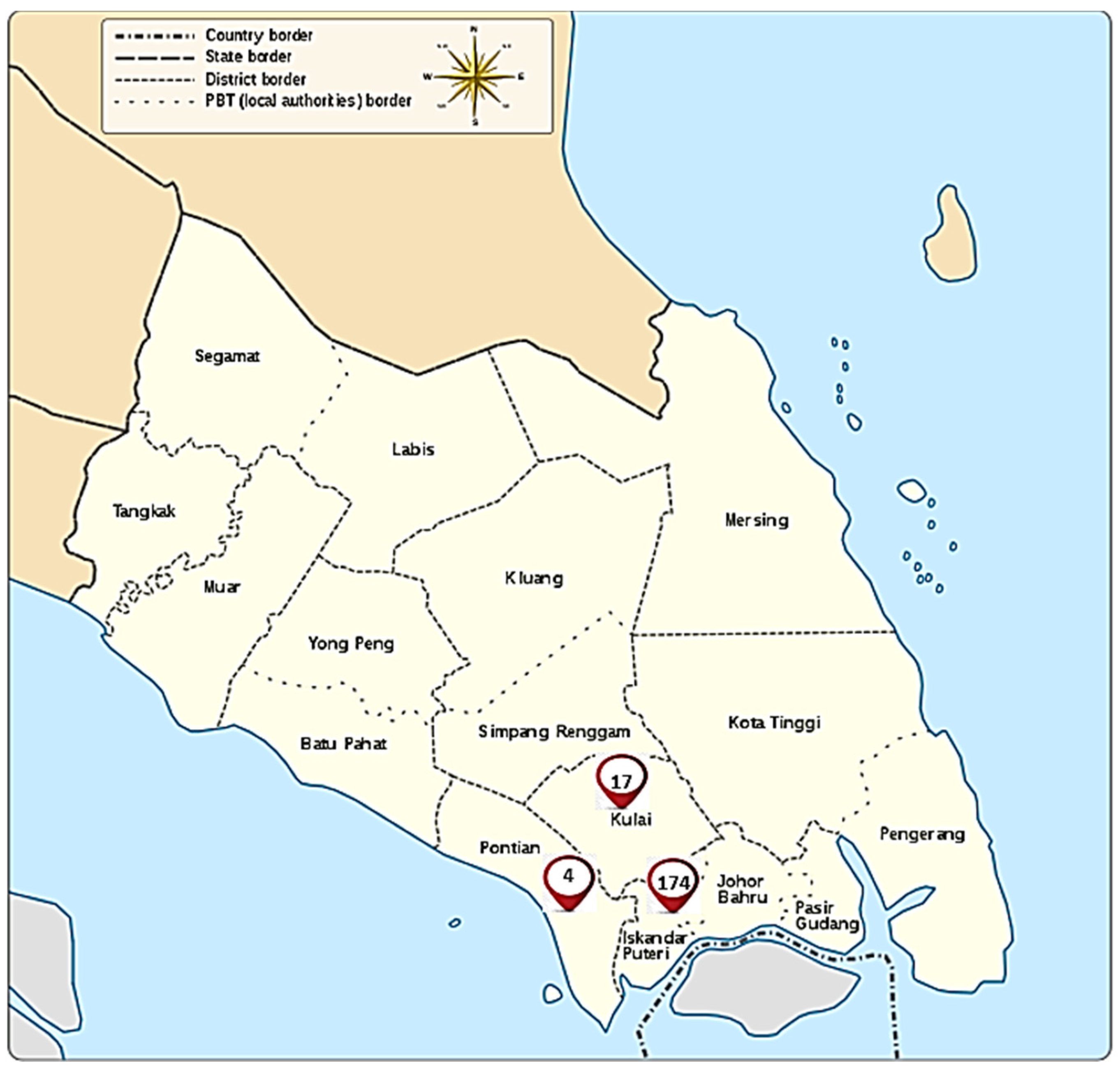
3.1. Site Description
3.2. Data Collection
3.3. Model Development Using Multilinear Regression Analysis (MRA)
4. Results
4.1. Measured Parameter Descriptive Outcomes
4.2. Developed Models Features
4.3. Model Validation
4.4. Models Application
5. Discussion
6. Conclusions
Author Contributions
Funding
Institutional Review Board Statement
Informed Consent Statement
Data Availability Statement
Conflicts of Interest
Appendix A

| Comparative ATS Results | Paired Differences | t | df | Sig. (2-Tailed) | ||||
|---|---|---|---|---|---|---|---|---|
| Mean | Std. Deviation | Std. Error Mean | 95% Confidence Interval of the Difference | |||||
| Lower | Upper | |||||||
| Observed ATS from MOM Versus Predicted ATS from Category A Model (km/h) with TV in veh/h | −0.450 | 1.90 | 0.425 | −1.34 | 0.441 | −1.05 | 19 | 0.304 |
| Observed ATS from MOM Versus Predicted ATS from Category B Model (km/h) with TV in pcu/h | −0.750 | 1.71 | 0.383 | −1.55 | 0.051 | −1.958 | 19 | 0.065 |
| Predicted ATS from Categories A and B Models (km/h) | 0.300 | 0.5712 | 0.127 | 0.0326 | 0.5673 | 2.349 | 19 | 0.030 |
| Comparative ATS Results | Paired Differences | t | df | Sig. (2-Tailed) | ||||
|---|---|---|---|---|---|---|---|---|
| Mean | Std. Deviation | Std. Error Mean | 95% Confidence Interval of the Difference | |||||
| Lower | Upper | |||||||
| Observed ATS from MOM Versus Predicted ATS from Category A Model (km/h) with TV in veh/h | −0.336 | 3.11 | 0.803 | −2.06 | 1.38 | −0.418 | 14 | 0.682 |
| Observed ATS from MOM Versus Predicted ATS from Category B Model (km/h) with TV in pcu/h | 0.703 | 3.216 | 0.830 | −1.078 | 2.485 | 0.847 | 14 | 0.411 |
| Predicted ATS from Categories A and B Models (km/h) | 0.367 | 1.049 | 0.271 | −0.214 | 0.949 | 1.356 | 14 | 0.197 |
| Comparative ATS Results | Paired Differences | t | df | Sig. (2-Tailed) | ||||
|---|---|---|---|---|---|---|---|---|
| Mean | Std. Deviation | Std. Error Mean | 95% Confidence Interval of the Difference | |||||
| Lower | Upper | |||||||
| Observed ATS from MOM Versus Predicted ATS from Category A Model (km/h) with TV in veh/h | −0.257 | 1.765 | 0.489 | −1.323 | 0.809 | −0.525 | 12 | 0.609 |
| Observed ATS from MOM Versus Predicted ATS from Category B Model (km/h) with TV in pcu/h | −1.257 | 1.932 | 0.536 | −2.425 | −0.089 | −2.345 | 12 | 0.037 |
| Predicted ATS from Categories A and B Models (km/h) | −1.000 | 0.408 | 0.113 | −1.247 | −0.753 | −8.832 | 12 | 0.000 |
| Comparative ATS Results | Paired Differences | t | df | Sig. (2-Tailed) | ||||
|---|---|---|---|---|---|---|---|---|
| Mean | Std. Deviation | Std. Error Mean | 95% Confidence Interval of the Difference | |||||
| Lower | Upper | |||||||
| Observed ATS from MOM Versus Predicted ATS from Category A Model (km/h) with TV in veh/h | −2.80 | 9.363 | 2.961 | −9.503 | 3.893 | −0.94 | 9 | 0.368 |
| Observed ATS from MOM Versus Predicted ATS from Category B Model (km/h) with TV in pcu/h | 3.229 | 9.450 | 2.988 | −3.531 | 9.989 | 1.081 | 9 | 0.308 |
| Predicted ATS from Categories A and B Models (km/h) | 0.424 | 0.339 | 0.107 | 0.181 | 0.667 | 3.951 | 9 | 0.003 |
| Comparative ATS Results | Paired Differences | t | df | Sig. (2-Tailed) | ||||
|---|---|---|---|---|---|---|---|---|
| Mean | Std. Deviation | Std. Error Mean | 95% Confidence Interval of the Difference | |||||
| Lower | Upper | |||||||
| Observed ATS from MOM Versus Predicted ATS from Category A Model (km/h) with TV in veh/h | 0.167 | 0.577 | 0.167 | −0.200 | 0.533 | 1.00 | 11 | 0.339 |
| Observed ATS from MOM Versus Predicted ATS from Category B Model (km/h) with TV in pcu/h | 0.667 | 0.651 | 0.188 | 0.253 | 1.081 | 3.546 | 11 | 0.005 |
| Predicted ATS from Categories A and B Models (km/h) | 0.500 | 0.522 | 0.151 | 0.168 | 0.832 | 3.317 | 11 | 0.007 |
References
- Cohen, S.; Zhang, M.Y. New Speed Flow Relationships for Road Network Planning in the Paris Region. In Traffic and Transportation Studies; American Society of Civil Engineers: Reston, VA, USA, 2002; pp. 389–396. [Google Scholar]
- Highway Planning Unit (HPU). Malaysian Highway Capacity Manual; Ministry of Works: Kuala Lumpur, Malaysia, 2006.
- Li, M.Z.F. A Generic Characterization of Equilibrium Speed-Flow Curves. Transp. Sci. 2008, 42, 220–235. [Google Scholar] [CrossRef]
- Chiguma, M.L. Analysis of Side Friction Impacts on Urban Road Links; Case Study, Dar-es-Salaam. Ph.D. Thesis, Royal Institute of Technology (KTH), Stockholm, Sweden, 2007. [Google Scholar]
- Transportation Research Board (TRB). Highway Capacity Manual; National Research Council: Washington, DC, USA, 2000. [Google Scholar]
- Li, M.Z.F. The role of speed–flow relationship in congestion pricing implementation with an application to Singapore. Transp. Res. Part B Methodol. 2002, 36, 731–754. [Google Scholar] [CrossRef]
- Hooper, E.; Chapman, L.; Quinn, A. The impact of precipitation on speed–flow relationships along a UK motorway corridor. Theor. Appl. Climatol. 2014, 117, 303–316. [Google Scholar] [CrossRef]
- Transportation Research Board (TRB). Highway Capacity Manual; National Research Council: Washington, DC, USA, 2010. [Google Scholar]
- Van Aerde, M.; Rakha, H. Multivariate calibration of single regime speed-flow-density relationships. In Pacific Rim TransTech Conference. 1995 Vehicle Navigation and Information Systems Conference Proceedings. 6th International VNIS. A Ride into the Future; IEEE: Piscataway, NJ, USA, 1995; pp. 334–341. [Google Scholar]
- Lum, K.M.; Fan, H.S.; Lam, S.H.; Olszewski, P. Speed-flow modeling of arterial roads in Singapore. J. Transp. Eng. 1998, 124, 213–222. [Google Scholar] [CrossRef]
- Chen, Y. Model of Traffic Speed-Flow Relationship at Signal Intersections. Open J. Appl. Sci. 2017, 7, 319–327. [Google Scholar] [CrossRef] [Green Version]
- Williams, J.C. Macroscopic Flow Models in Traffic Flow Theory; US Federal Highway Administration: Washington, DC, USA, 2001.
- Branston, D. Link capacity functions: A review. Transp. Res. 1976, 10, 223–236. [Google Scholar] [CrossRef]
- Campbell, E.W.; Keefer, L.E.; Adams, R.W. A method for predicting speeds through signalized street sections. Highw. Res. Board Bull. 1959, 230, 112–125. [Google Scholar]
- Smeed, R.I. Road capacity of city centres. Traffic Eng. Control. 1966, 8, 455–458. [Google Scholar]
- Ardekani, S.A.; Williams, J.C.; Bahat, S. Influence of Urban Network Features on Quality of Traffic Service. Transp. Res. Rec. 1992, 1358. [Google Scholar]
- Wardrop, J.G. Journey speed and flow in central urban areas. Traffic Eng. Control 1968, 9, 528–532. [Google Scholar]
- Zahavi, Y. Traffic performance evaluation of road networks by the α-relationship, Part 1. Traffic Eng. Control 1972, 14, 292–293. [Google Scholar]
- Zahavi, Y. Traffic performance evaluation of road networks by the α-relationship, Part 2. Traffic Eng. Control 1972, 14, 228–231. [Google Scholar]
- Leong, L.V.; Azai, T.A.; Goh, W.C.; Mahdi, M.B. The development and assessment of free-flow speed models under heterogeneous traffic in facilitating sustainable inter urban multilane highways. Sustainability 2020, 12, 3445. [Google Scholar] [CrossRef] [Green Version]
- Prahara, E.; Prasetya, R.A. Speed–volume relationship and headway distribution analysis of motorcycle (case study: Teuku Nyak Arief Road). In IOP Conference Series: Earth and Environmental Science (vol. 106, no. 1); IOP Publishing: Jakarta, Indonesia, 2018. [Google Scholar]
- Yasanthi, R.G.N.; Mehran, B. Modeling free-flow speed variations under adverse road-weather conditions: Case of cold region highways. Case Stud. Transp. Policy 2020, 8, 22–30. [Google Scholar] [CrossRef]
- Chathoth, V.; Asaithambi, G. Modeling free-flow speeds on undivided roads in mixed traffic with weak lane discipline. Transp. Res. Rec. 2018, 2672, 105–117. [Google Scholar] [CrossRef]
- Bassani, M.; Dalmazzo, D.; Marinelli, G.; Cirillo, C. The effects of road geometrics and traffic regulations on driver-preferred speeds in northern Italy. An exploratory analysis. Transp. Res. Part F Traffic Psychol. Behav. 2014, 25, 10–26. [Google Scholar] [CrossRef]
- Eluru, N.; Chakour, V.; Chamberlain, M.; Miranda-Moreno, L.F. Modeling vehicle operating speed on urban roads in Montreal: A panel mixed ordered probit fractional split model. Accid. Anal. Prev. 2013, 59, 125–134. [Google Scholar] [CrossRef]
- Wang, J. Operating Speed Models for Low Speed Urban Environments Based on In-Vehicle GPS Data. Ph.D. Thesis, Georgia Institute of Technology, Atlanta, GA, USA, 2006. [Google Scholar]
- Schueller, H. Modeling Speeds and Accidents on Urban Streets. In Proceedings of the ICTIS, First International Conference on Transportation Information and Safety, Wuhan, China, 30 June–2 July 2011; pp. 830–836. [Google Scholar]
- Herwandy, A. Road Performance Analysis with Median and without Median on the Road of A. Yani Satui. CERUCUK 2020, 4, 17–32. [Google Scholar] [CrossRef]
- Asma, A.T. Empirical Models for Estimating Automobiles Running Speeds on Urban Streets. Ph.D. Thesis, George Mason University, Fairfax, VA, USA, 2007. [Google Scholar]
- Juhász, M.; Mátrai, T.; Koren, C. Forecasting travel time reliability in urban road transport. Arch. Transp. 2017, 43, 53–67. [Google Scholar] [CrossRef] [Green Version]
- Smock, R. An iterative assignment approach to capacity restraint on arterial networks. Highw. Res. Board Bull. 1962, 347, 60–66. [Google Scholar]
- Juhász, M.; Koren, C.; Mátrai, T. Analysing the Speed-flow Relationship in Urban Road Traffic. Acta Tech. Jaurinensis 2016, 9, 128–139. [Google Scholar] [CrossRef] [Green Version]
- Geroliminis, N. A Macroscopic Fundamental Diagram of Urban Traffic: Recent Findings. In Proceedings of the Symposium on the Fundamental Diagram: 75 Years, Woods Hole, MA, USA, 8–10 July 2008. [Google Scholar]
- Transportation Research Board (TRB). Highway Capacity Manual; National Research Council: Washington, DC, USA, 1985. [Google Scholar]
- Pei, X.; Wong, S.C.; Li, Y.C.; Sze, N.N. Full Bayesian Method for the Development of Speed Models: Applications of GPS Probe Data. J. Transp. Eng. 2012, 138, 1188–1195. [Google Scholar] [CrossRef]
- Ali, A.T.; Venigalla, M.M.; Flannery, A. Estimating Running Time on Urban Street. In Proceedings of the 3rd Urban Street Symposium, Seattle, WA, USA, 24–27 June 2007; Volume 1738, pp. 24–27. [Google Scholar]
- Munawar, A. Speed and capacity for urban roads, Indonesian experience. Procedia-Soc. Behav. Sci. 2011, 16, 382–387. [Google Scholar] [CrossRef] [Green Version]
- Salini, S.; George, S.; Ashalatha, R. Effect of Side Frictions on Traffic Characteristics of Urban Arterials. Transp. Res. Procedia 2016, 17, 636–643. [Google Scholar] [CrossRef]
- Yang, J.; Xu, J.; Gao, C.; Bai, G.; Xie, L.; Li, M. Modeling of the relationship between speed limit and characteristic speed of expressway traffic flow. Sustainability 2019, 11, 4621. [Google Scholar] [CrossRef] [Green Version]
- Jomnonkwao, S.; Uttra, S.; Ratanavaraha, V. Forecasting road traffic deaths in Thailand: Applications of time-series, curve estimation, multiple linear regression, and path analysis models. Sustainability 2020, 12, 395. [Google Scholar] [CrossRef] [Green Version]
- Jin, S.; Shen, L.; Liu, M.; Ma, D. Modelling speed–flow relationships for bicycle traffic flow. Proc. Inst. Civ. Eng. Transp. 2017, 170, 194–204. [Google Scholar] [CrossRef]
- Qu, X.; Zhang, J.; Wang, S. On the stochastic fundamental diagram for freeway traffic: Model development, analytical properties, validation, and extensive applications. Transp. Res. Part B Methodol. 2017, 104, 256–271. [Google Scholar] [CrossRef]
- Golob, T.F.; Recker, W.W. Relationships among urban freeway accidents, traffic flow, weather, and lighting conditions. J. Transp. Eng. 2003, 129, 342–353. [Google Scholar] [CrossRef]
- Sulistio, H. Effect of Traffic Flow, Proportion of Motorcycle, Speed, Lane Width, and the Availabilities of Median and Shoulder on Motorcycle Accidents at Urban Roads in Indonesia. Open Transp. J. 2018, 12, 1–7. [Google Scholar] [CrossRef]
- Hair, J.; Black, W.; Babin, B.; Anderson, R.; Tatham, R. Multivariate Data Analysis, 5th ed.; Pearson Prentice Hall: Hoboken, NJ, USA, 2005. [Google Scholar]
- Kutner, M.H.; Nachtsheim, C.J.; Neter, J.; Li, W. Applied Linear Statistical Models; McGraw-Hill Irwin: Boston, MA, USA, 1996; Volume 5. [Google Scholar]
- Jain, G.V.; Agrawal, R.; Sharma, K.; Bhanderi, R.J.; Jayaprasad, P. Evaluation of Urban Road Network Using Geoinformatics—A Case Study of Surat City. Int. J. Remote Sens. Geosci. 2014, 3, 47–53. [Google Scholar]
- Barua, S.; Das, A.; Hossain, M.J. Estimation of Traffic Density to Compare Speed- Density Models with Moving Observer Data. Int. J. Res. Eng. Technol. 2015, 4, 471–474. [Google Scholar]
- Hall, F.L. Traffic Stream Characteristics; US Federal Highway Administration: Washington, DC, USA, 1996.
- Al-Bahr, T.M.; Puan, O.C. Speed-Flow Relationship for Urban Roads: A Preliminary Assessment. Adv. Sci. Lett. 2018, 24, 4172–4176. [Google Scholar] [CrossRef]
- Al-Bahr, T.M.; Puan, O.C.; Hassan, S.A.; Idham, M.K.; Ismail, C.R. Parameters affecting fluctuation in traffic stream on urban roads. In IOP Conference Series: Materials Science and Engineering; IOP Puplishing: Bristol, UK, 2019; p. 527. [Google Scholar]
- Raqib, A.; Hashim, W.; Ibrahim, W.; Farhan, A.; Sadullah, M. Estimating Travel Time of Arterial Road Using Car Chasing Method and Moving Observer Method. J. Transp. Sci. Soc. Malays. 2005, 1, 77–87. [Google Scholar]
- Triola, M.F. Elementary Statistics; Pearson/Addison-Wesley: Reading, MA, USA, 2006. [Google Scholar]
- Lind, D.A.; Marchal, W.G.; Wathen, S.A.; Waite, C.A. Basic Statistics for Business & Economics; McGraw-Hill/Irwin: Boston, MA, USA, 2006. [Google Scholar]
- Highway Planning Unit (HPU). Malaysian Highway Capacity Study Stage 3 (Inter-Urban); Ministry of Works: Kuala Lumpur, Malaysia, 2011.


| Ref. | Model Equation |
|---|---|
| Campbell, 1959 [14] | |
| Smock, 1962 [31] | |
| Wardrop 1968 [17] | |
| Lum et al. (1998) [10] | |
| Juhász, Koren and Mátrai (2016) [32] | |
| Chen (2017) [11] |
| No. | Name of Parameters | Symbol of Parameters | Measurement Unit | Type of Variable | Parameter Group Type | Method of Data Collection | |
|---|---|---|---|---|---|---|---|
| 1 | Average Travel Speed | ATS | km/h | Dependent variable | -- | Moving Observer Method (MOM) | |
| 2 | Traffic Volume (TV) | Traffic Volume (TV) for all Vehicle Classes | TVveh/h | veh/h | Independent variable | -- | |
| 3 | Equivalent Traffic Volume (TV) for Passenger Car | TVpcu/h | pcu/h | -- | |||
| 4 | Traffic Calming Speed Density | TCSD | No./km | Type I parameters (Longitudinal Parameters, LP) | Visual Direct Measurement (Natural Human Eye) | ||
| 5 | Intersection Density | IntersD | |||||
| 6 | Access Driveway Density | AccessD | |||||
| 7 | Right-turn Driveway Density | RTD | |||||
| 8 | Median Existence | M | 0 = No Median 1 = Have Median | Type II parameter (Cross-sectional Parameters, CSP) | |||
| 9 | Side Friction | SF | 0 = Low, 1 = High | ||||
| 10 | Number of Lane | NL | 1 = One lane 2 = Two lanes 3 = Three lanes | ||||
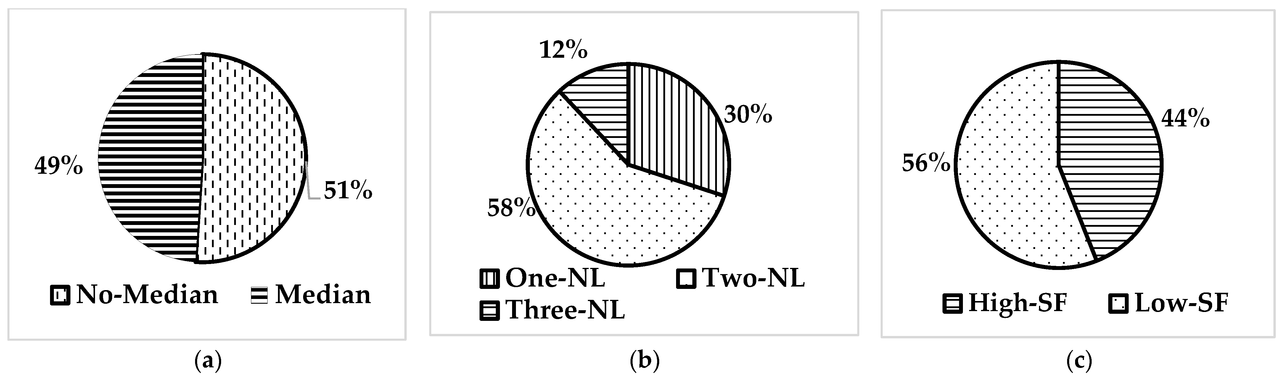
| Group No. | Cross-Sectional Parameters Condition of the Surveyed Urban Roads (SUR) Groups (Group Symbol) | Number of SUR in Group | Road’s Group Proportion (%) |
|---|---|---|---|
| 1 | No Median, One Lane Number, Low Side Friction [M0, NL1, SF0] | 37 | 18.78 |
| 2 | No Median, One Lane Number, High Side Friction [M0, NL1, SF1] | 22 | 11.17 |
| 3 | No Median, Two Lane Number, Low Side Friction [M0, NL2, SF0] | 17 | 8.63 |
| 4 | No Median, Two Lane Number, High Side Friction [M0, NL2, SF1] | 25 | 12.69 |
| 5 | Have Median, Two Lane Number, Low Side Friction [M1, NL2, SF0] | 36 | 18.27 |
| 6 | Have Median, Two Lane Number, High Side Friction [M1, NL2, SF1] | 37 | 18.78 |
| 7 | Have Median, Three Lane Number, Low Side Friction [M1, NL3, SF0] | 21 | 10.66 |
| 8 | Have Median, Three Lane Number, High Side Friction [M1, NL3, SF1] | 2 | 1.02 |
| 9 | No Median, Three Lane Number, Low Side Friction [M0, NL3, SF0] | 0 | 0 |
| 10 | No Median, Three Lane Number, High Side Friction [M0, NL3, SF1] | 0 | 0 |
| 11 | Have Median, One Lane Number, Low Side Friction [M1, NL1, SF0] | 0 | 0 |
| 12 | Have Median, One Lane Number, High Side Friction [M1, NL1, SF1] | 0 | 0 |
| All surveyed urban roads segments | 197 | 100% | |
| Variables | No. of SUR | Mean | Range | Median | Standard Deviation |
|---|---|---|---|---|---|
| ATS (km/h) | 197 | 29.71 | (11–56) | 30.0 | 7.01 |
| TV (veh/h) | 197 | 718 | (27–2957) | 517 | 594 |
| TCSD (No./km) | 197 | 3.36 | (35.87–0) | 2.30 | 4.27 |
| AccessD (No./km) | 197 | 4.73 | (0–17.94) | 4.32 | 3.04 |
| IntersD (No./km) | 197 | 1.94 | (0–8.97) | 1.72 | 1.50 |
| RTD (No./km) | 101 | 4.90 | (0–15.77) | 4.43 | 3.22 |
| No. | CSP Category | Group A (TV in veh/h) | Group B (TV in pcu/h) | Regression Results (√ = Success), (✕ = Fail) | ||||
|---|---|---|---|---|---|---|---|---|
| Model’s Equation | R2 (Standard Error) | F-Test Value (Significance) | Model’s Equation | R2 (Standard Error) | F-Test Value (Significance) | |||
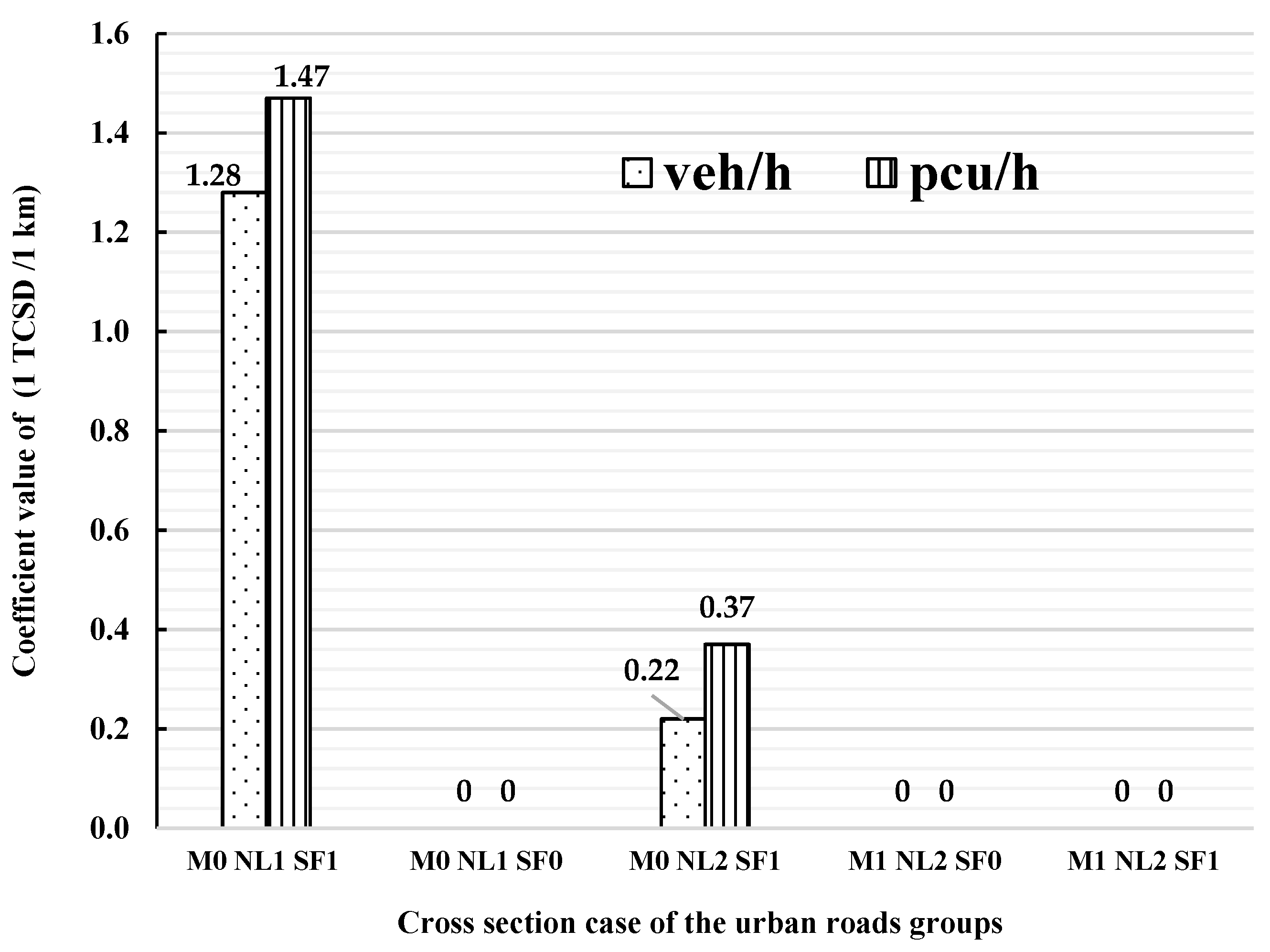
| 1 | [M0, NL1, SF0] | ATS = 39.70 − 0.017 TV − 0.26 AccessD | 0.71 (1.87) | 42.53 (0.00) | ATS = 39.39 − 0.02 TV − 0.26 AccessD | 0.78 (1.59) | 58.20 (0.00) | √ |
| 2 | [M0, NL1, SF1] | ATS = 34.785 − 0.01 TV − 1.28 TSCD − 1.26 IntersD | 0.87 (2.14) | 40.85 (0.00) | ATS = 34.50 − 0.01 TV − 1.47 TSCD − 1.41 IntersD | 0.87 (2.19) | 38.66 (0.00) | √ |
| 3 | [M0, NL2. SF1] | ATS = 32.05 − 0.012 TV − 0.22 TCSD | 0.94 (0.64) | 168.34 (0.00) | ATS = 31.8 − 0.011 TV − 0.37 TCSD | 0.87 (0.87) | 75.74 (0.00) | √ |
| 4 | [M1, NL2, SF0] | ATS = 40.79 − 0.01 TV | 0.94 (0.64) | 59.06 (0.00) | ATS = 40.26 − 0.01 TV | 0.62 (3.37) | 55.19 (0.00) | √ |
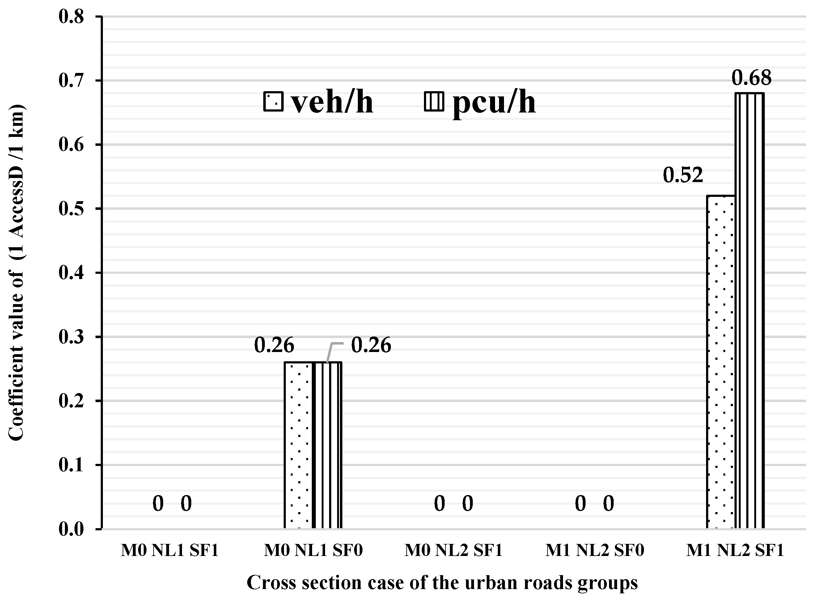
| 5 | [M1, NL2, SF1] | ATS = 37.47 − 0.01 TV − 0.52 AccessD | 0.98 (0.98) | 749.86 (0.00) | ATS = 37.21 − 0.01 TV − 0.68 AccessD | 0.96 (1.27) | 446.46 (0.00) | √ |
| 6 | [M0, NL2, SF0] | ATS = 18.47 − 0.003 TV + 0.76TCSD + 0.52 AccessD + 0.50 IntersD − 0.21 RTD | 0.50 (2.22) | 2.22 (0.12) | ATS = 18.47 − 0.003 TV + 0.76 TCSD + 0.52 AccessD + 0.50 IntersD − 0.21 RTD | 0.50 (2.22) | 2.22 (0.12) | ✕ |
| 7 | [M1, NL3, SF0] | ATS = 35.87 + 1.27 TCSD | 0.13 (8.18) | 2.94 (0.10) | ATS = 35.87 + 1.27 TCSD | 0.13 (8.18) | 2.94 (0.10) | ✕ |
| Group of Surveyed Urban Roads (SUR) | Group 1 | Group 2 | Group 3 | Final Model Adopted | |||
|---|---|---|---|---|---|---|---|
| Paired t-Test between the Observed ATS Using MOM and the Estimated ATS Using Model A (veh/h) | Paired t-Test between the Observed ATS Using MOM and the Estimated ATS Using Model B (pcu/h) | Paired t-Test between the Estimated ATS Using Model A (veh/h) and the Estimated ATS Using Model B (pcu/h) | |||||
| t-Value | p-Value | t-Value | p-Value | t-Value | p-Value | ||
| [M0, NL1, SF0] | −1.05 | 0.304 * | −1.958 | 0.065 * | 2.35 | 0.03 | Model B (pcu/h) |
| [M0, NL1, SF1] | −0.418 | 0.682 * | 0.847 | 0.411 * | 1.356 | 0.197 * | Model A (veh/h) |
| [M0, NL2 SF1] | −0.525 | 0.609 * | −2.35 | 0.037 | Ineligible | Ineligible | Model A (veh/h) |
| [M1, NL2, SF0] | −0.94 | 0.368 * | 1.081 | 0.308 * | 3.95 | 0.003 | Model B (pcu/h) |
| [M1, NL2, SF1] | 1.00 | 0.339 * | 3.546 | 0.005 | Ineligible | Ineligible | Model A (veh/h) |
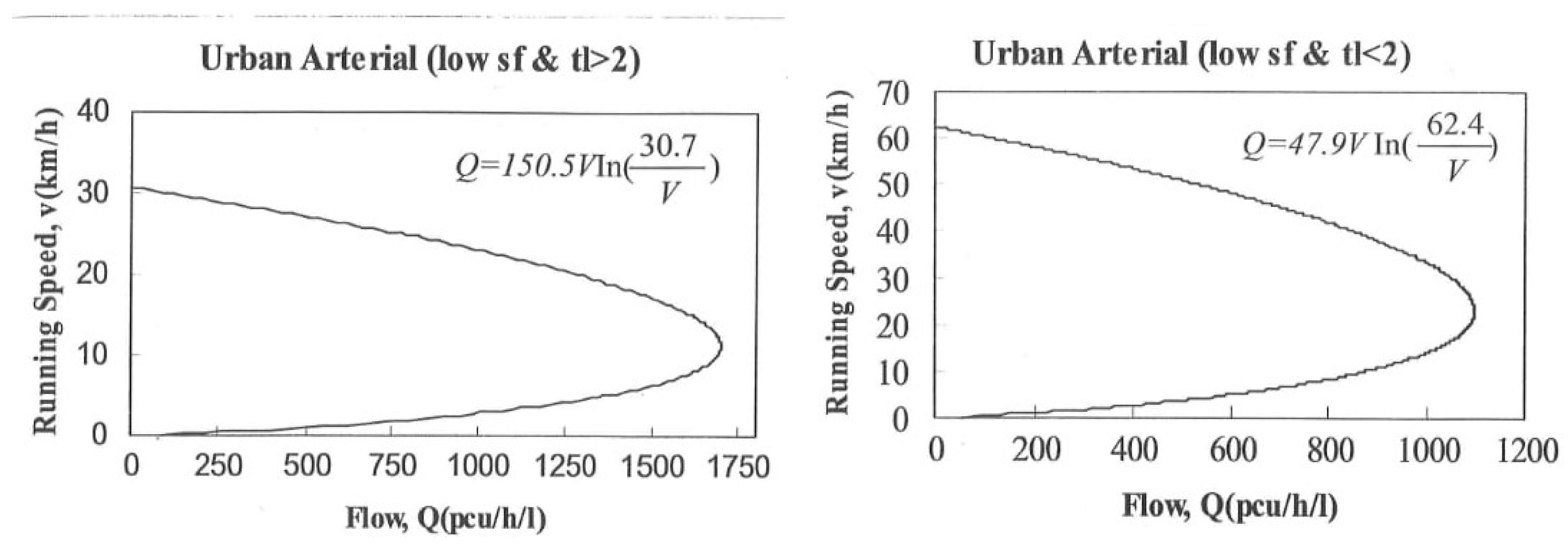
| No. | Roads’ Group Features | Max. FFS (km/h) | Type of Longitudinal Parameters (LP) and Range of Values (No./km) | Range of Traffic Volume (TV) (veh/h)/(pcu/h) | |
|---|---|---|---|---|---|
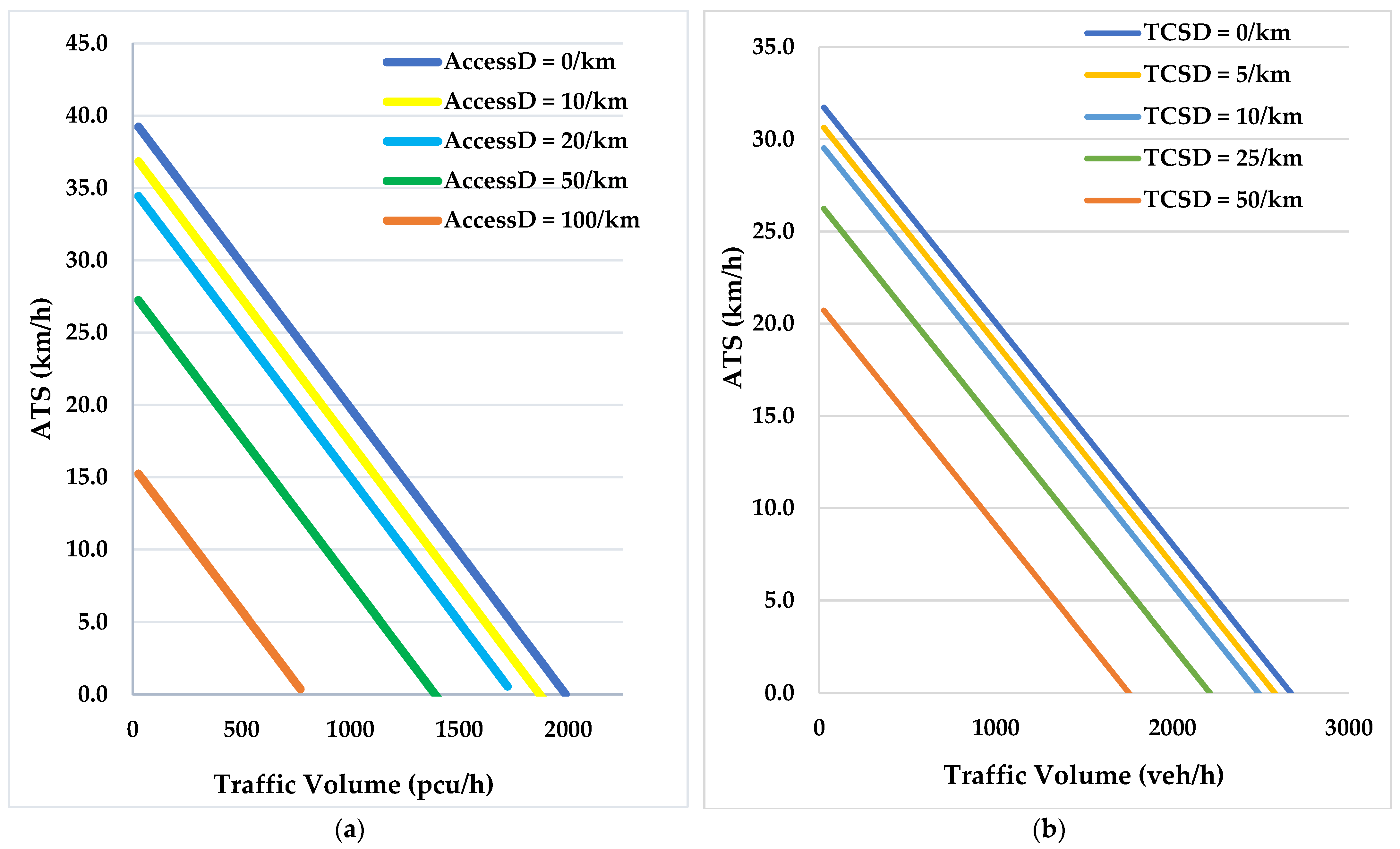
| 1 | [M0, NL1, SF0] (Model B) | 39.7 | AccessD (0, 10, 20, 50, 100) | (0–1989) | |
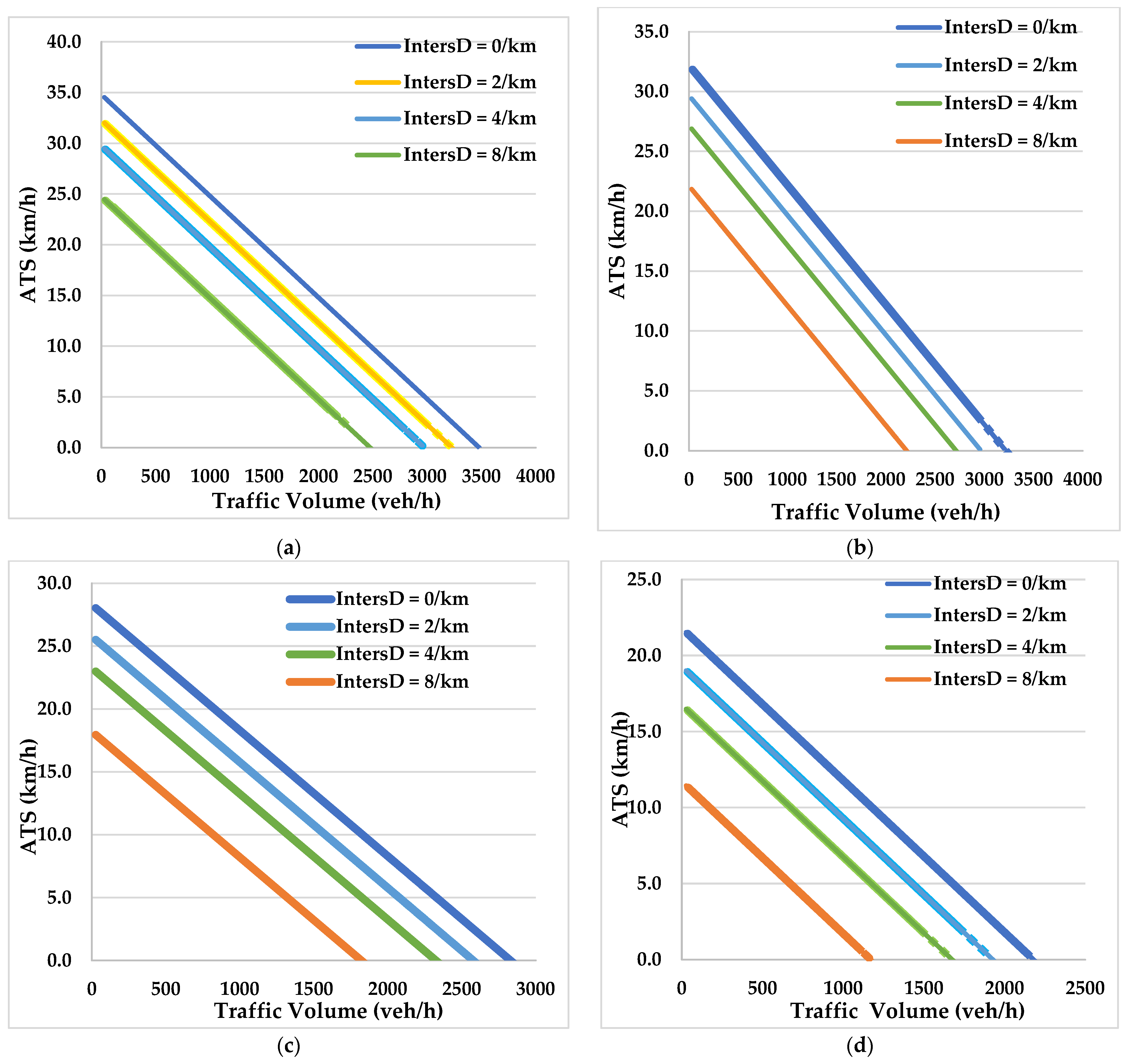
| 2 | [M0, NL2, SF1] (Model A) | 32.14 | TCSD (0, 5, 10, 25, 50) | (0–2650) | |
| 3 | [M1, NL2, SF1] (Model A) | 37.47 | AccessD (0, 10, 20, 40) | (0–3730) | |
| 4 | [M1, NL2, SF0] (Model B) | 40.77 | (No-Longitude Parameters) | (0–4077) | |
| 5 | [M0, NL1, SF1] (Model A) | 34.82 | TCSD (0, 2, 5, 10) | IntersD (0, 2, 4, 8) | (0–3482) |
Publisher’s Note: MDPI stays neutral with regard to jurisdictional claims in published maps and institutional affiliations. |
© 2022 by the authors. Licensee MDPI, Basel, Switzerland. This article is an open access article distributed under the terms and conditions of the Creative Commons Attribution (CC BY) license (https://creativecommons.org/licenses/by/4.0/).
Share and Cite
Al-Bahr, T.M.; Hassan, S.A.; Puan, O.C.; Mashros, N.; Sukor, N.S.A. Speed-Flow-Geometric Relationship for Urban Roads Network. Appl. Sci. 2022, 12, 4231. https://doi.org/10.3390/app12094231
Al-Bahr TM, Hassan SA, Puan OC, Mashros N, Sukor NSA. Speed-Flow-Geometric Relationship for Urban Roads Network. Applied Sciences. 2022; 12(9):4231. https://doi.org/10.3390/app12094231
Chicago/Turabian StyleAl-Bahr, Tareq M., Sitti Asmah Hassan, Othman Che Puan, Nordiana Mashros, and Nur Sabahiah Abdul Sukor. 2022. "Speed-Flow-Geometric Relationship for Urban Roads Network" Applied Sciences 12, no. 9: 4231. https://doi.org/10.3390/app12094231