An Efficient Parallel Implementation of the Runge–Kutta Discontinuous Galerkin Method with Weighted Essentially Non-Oscillatory Limiters on Three-Dimensional Unstructured Meshes

Abstract

In computational fluid dynamics, high-order solvers suitable for three-dimensional unstructured meshes are attractive but are less developed than other methods. In this article, we provide the formulation and a parallel implementation of the Runge–Kutta discontinuous Galerkin finite element method with weighted essentially non-oscillatory limiters, which are compact and effective for suppressing numerical oscillations near discontinuities. In our experiments, high-order solvers do outperform their low-order counterparts in accuracy and the efficient parallel implementation makes the time cost affordable for large problems. Such high-order parallel solvers are efficient tools for solving conservative laws including the Euler system that models inviscid compressible flows.

1. Introduction

Most of the computational fluid dynamics (CFD) solvers currently used in aerospace engineering are based on schemes using finite volume (FV) methods, which are more suitable than schemes using finite difference (FD) methods for unstructured meshes. However, FV schemes usually have only second-order spatial accuracy, due to the difficulty of handling irregular local stencils, whose sizes grows rapidly as the order of accuracy increases. In high-order FV schemes, the local stencil of a cell is made up of the cell and the cell’s neighbors, and the neighbors’ neighbors, and so on. To ease the development of high-order schemes for unstructured meshes, it is better to use finite element (FE) methods whose local stencils are much more compact than those of FV schemes. One family of such compact high-order schemes suitable for unstructured meshes are called the discontinuous Galerkin (DG) methods, which assume continuous approximation in each cell (like classic FE methods), but allow discontinuities to exist on cell boundaries (like classic FV methods). Such an assumption gives scheme designers more freedom on choosing the basis for each cell, such as orthogonal functions which lead to modal DG methods, and Lagrange polynomials which lead to nodal DG methods [1]. The original DG method was introduced by Reed and Hill [2] for solving the neutron transport equation, which is a linear problem contains only first-order spatial derivatives. For nonlinear conservation laws, Chavent and Salzano [3] made the first attempt of using a DG method to discretize in space and using the explicit Euler method for time discretization. This scheme is second-order accurate in space but only first-order accurate in time. To improve the accuracy of time discretization, Cockburn and Shu [4] replace the first-order Euler method with a special second-order Runge–Kutta (RK) method [5,6], which is explicit and total variation diminishing (TVD). This is the first successful Runge–Kutta discontinuous Galerkin (RKDG) method, which is high-order accurate both in space and time, for scalar conservation laws. This RKDG method was soon extended to one-dimensional system case [7], multi-dimensional scalar case [8] and multi-dimensional system case [9], which includes the Euler system that models inviscid compressible flows. Nearly the same time (late 1990s), the DG methods were also extended to the Navier–Stokes system that governs viscous flows. Bassi and Rebay [10] made the first attempt to apply the DG idea to both the unknowns and their gradients for solving the Navier–Stokes equations. This method was then generalized by Cockburn and Shu [11] to the family of local discontinuous Galerkin (LDG) methods, which extends the RKDG methods from conversation laws to convection-dominated problems. One may refer to [12], which is a comprehensive review article on this topic. In the rest of this article, we will only study the RKDG methods for conservation laws that are purely hyperbolic. In Section 2.1 and Section 2.3, we will give a matrix formed formulation of the RKDG method for solving three-dimensional conservation law systems.

When solving hyperbolic problems, limiting procedures, or limiters for short, are necessary for suppressing numerical oscillations that might occur near discontinuities (known as the Gibbs phenomenon [13]). For FD and FV schemes, there is the monotonic upstream-centered scheme for conservation laws (MUSCL) [14,15,16,17], which could achieve third-order accuracy when used with caution. However, it is not directly applicable to FE schemes. Besides the RKDG formulations, there is another important contribution made by [8,9], which is proposing the generalized slope limiters for multi-dimensional problems. These minmod type limiters, together with TVD RK methods, makes the high-order solutions free from non-physical oscillation, but tend to reduce the order of accuracy in smooth regions. To overcome this drawback, the essentially non-oscillatory (ENO) [18] and weighted ENO (WENO) [19] limiting procedures were introduced. Both of them can maintain high-order accuracy in smooth regions but essentially suppress spurious oscillations near discontinuities. The first attempt of making such limiters suitable for unstructured meshes was to incorporate a WENO reconstruction procedure into high-order FV schemes [20]. Similar ideas were later adopted for DG methods [21,22] at the cost of sacrificing the compactness of DG methods. Compact versions of WENO limiters suitable for DG methods only occurred in the last ten years [23,24,25] and most of them are only formulated for two-dimensional meshes. In Section 2.2, we will give a unified formulation of some compact WENO limiters for both two- and three-dimensional RKDG methods on unstructured meshes.

The two-dimensional version of the algorithms described in Section 2.1, Section 2.2 and Section 2.3 has been proposed for nearly ten years, but few three-dimensional or real engineering applications have been reported so far. One reason is that the amount of computational resources cost by each cell grows rapidly as the order of accuracy or the dimension of space increases. Fortunately, both RKDG methods and WENO limiters use highly compact stencils and there is no global algebraic equation to be solved (as in FD and FV schemes). Based on these facts, parallel computing using domain decomposition can be applied for accelerating computation in a very natural way. Currently, we have not seen any parallel implementation of RKDG methods with WENO limiters for three-dimensional unstructured meshes. However, there are some frequently referenced works existing in the literature, which measured the parallel efficiencies of their DG methods. Biswas, Devine and Flaherty [26] performed some tests of their one- and two-dimensional DG solvers for linear scalar problems on uniform structured meshes. They achieved excellent parallel efficiencies, which were over $99\%$ for pure solution time (without I/O) and at least $89\%$ for total running time. Bey, Patra and Oden [27] tested their DG solvers for linear conservation laws on both structured (uniform) and unstructured ($hp$-adaptive) meshes. They obtained nearly optimal speedups when the number of interior elements is sufficiently larger than that of subdomain boundary elements. Recently, Chalmers et al. [28] implemented their DG solver for two-dimensional Navier–Stokes equations using MPI/OpenMP hybrid parallelism and achieved good scalability on a uniform mesh with only quadrilateral elements. None of them show the parallel performance of DG solvers on three-dimensional unstructured meshes. In this article, we incorporate unstructured mesh partitioning and message passing into the algorithms and implement them on top of publicly available libraries to support parallel execution. To partition a three-dimensional unstructured mesh, we use the application programming interface (API) provided by the Metis library [29]. To send and receive messages, we use the message passing interface (MPI) [30], which is the de facto industry standard of distributed memory parallelization. We will give the details of these parallel programming techniques in Section 2.4.

2. Methods

2.1. Spatial Discretization

The differential form of a conservation law system in a three-dimensional space could be written as

$${\partial }_t\underline{U}+{\partial }_x\underline{F^x}+{\partial }_y\underline{F^y}+{\partial }_z\underline{F^z}=\underline{O}$$

(1)

in which

• ${\partial }_t,{\partial }_x,{\partial }_y,{\partial }_z$ represent $\frac{\partial }{\partial t},\frac{\partial }{\partial x},\frac{\partial }{\partial y},\frac{\partial }{\partial z}$, respectively;
• $\underline{U}$ is a $K\times 1$ matrix of unknowns, each row of which is a scalar function depending on position $\overrightarrow{x}$ and time t;
• $\underline{F^{\mu }}$ (where $\mu =x,y,z$) is also a $K\times 1$ matrix, which is the dot-product of the flux $\underline{\overrightarrow{F}}$ (whose value depends on $\underline{U}$) and ${\overrightarrow{e}}_{\mu }$ (which is an unit vector along the positive direction of the $\mu$-axis);
• $\underline{O}$ is a $K\times 1$ matrix of 0’s.

This differential equation could be turned into an integral equation, by multiplying both sides with an arbitrary function $V(\overrightarrow{x})$ and integrating the product on an arbitrary control volume $\Omega$:

$${\int }_{\Omega }\left({\partial }_t\underline{U}+\nabla ·\underline{\overrightarrow{F}}\right)V=\underline{O}.$$

To weaken the smoothness requirements on $\underline{\overrightarrow{F}}$, we apply integral by parts and Gauss’s divergence theorem to it, which will lead to the weak form of Equation (1):

$${\int }_{\Omega }\left({\partial }_t\underline{U}-\underline{\overrightarrow{F}}·\nabla V\right)+{\int }_{\partial \Omega }\left(\overrightarrow{\nu }·\underline{\overrightarrow{F}}\right)V=\underline{O},$$

(2)

where $\overrightarrow{\nu }$ is the outer normal unit vector of the control surface $\partial \Omega$ (which is the boundary of $\Omega$).

To introduce spatial discretization for Equation (2), we choose the linear space spanned by polynomials up to the p-th degree over $\Omega$, denoted as ${\mathcal{V}}^p(\Omega )$, as the approximation space. Let $\underline{\varphi }\left(\overrightarrow{x}\right)=\left[\begin{array}{c}{\varphi }_1\left(\overrightarrow{x}\right)\cdots {\varphi }_L\left(\overrightarrow{x}\right)\end{array}\right]$ be a basis of ${\mathcal{V}}^p(\Omega )$, in this article, we choose

$${\varphi }_1\left(\overrightarrow{x}\right)=1,\left[\begin{array}{c}{\varphi }_2\left(\overrightarrow{x}\right)\\ {\varphi }_3\left(\overrightarrow{x}\right)\\ {\varphi }_4\left(\overrightarrow{x}\right)\end{array}\right]=\left[\begin{array}{c}x-x_0\\ y-y_0\\ z-z_0\end{array}\right],\left[\begin{array}{c}{\varphi }_5\left(\overrightarrow{x}\right)\\ {\varphi }_6\left(\overrightarrow{x}\right)\\ {\varphi }_7\left(\overrightarrow{x}\right)\\ {\varphi }_8\left(\overrightarrow{x}\right)\\ {\varphi }_9\left(\overrightarrow{x}\right)\\ {\varphi }_{10}\left(\overrightarrow{x}\right)\end{array}\right]=\left[\begin{array}{c}(x-x_0)(x-x_0)\\ (x-x_0)(y-y_0)\\ (x-x_0)(z-z_0)\\ (y-y_0)(y-y_0)\\ (y-y_0)(z-z_0)\\ (z-z_0)(z-z_0)\end{array}\right],\cdots ,$$

in which $(x_0,y_0,z_0)$ is the geometric center of $\Omega$. Then $\underline{U}$ and V could be approximated as

$$\underline{U}(\overrightarrow{x},t)\approx {\underline{U}}^h(\overrightarrow{x},t)=\sum _{l=1}^L{\widehat{\underline{U}}}_l\left(t\right){\varphi }_l\left(\overrightarrow{x}\right),V\left(\overrightarrow{x}\right)\approx V^h\left(\overrightarrow{x}\right)=\sum _{l=1}^L{\widehat{V}}_l{\varphi }_l\left(\overrightarrow{x}\right),$$

where each ${\widehat{\underline{U}}}_l\left(t\right)$ is a $K\times 1$ matrix of temporal functions, and each ${\widehat{V}}_l$ is a constant number (which is arbitrary since $V\left(\overrightarrow{x}\right)$ is arbitrary). Substitute them into the weak form (Equation (1)), we obtain   

$$\sum _l{\widehat{V}}_l\left[\sum _k\left({\int }_{\Omega }{\varphi }_l{\varphi }_k\right){\underline{\widehat{U}}}_{k}t+{\int }_{\Omega }\left(\nabla {\varphi }_l\right)·\underline{\overrightarrow{F}}\left({\underline{U}}^h\right)+{\oint }_{\partial \Omega }{\varphi }_l\underline{F^{\nu }}\left({\underline{U}}_{\mathrm{I}}^h,{\underline{U}}_{\mathrm{O}}^h\right)\right]=\underline{O}$$

(3)

where $\overrightarrow{\nu }·\underline{\overrightarrow{F}}=:\underline{F^{\nu }}$ is the normal flux on $\partial \Omega$, whose value could be solved from ${\underline{U}}_{\mathrm{I}}^h$ (the approximated inner-side state) and ${\underline{U}}_{\mathrm{O}}^h$ (the approximated outer-side state). We implement this procedure as an independent module called the Riemann solver of the conservation law (Equation (1)), see [31] for details.

Recall the arbitrariness of ${\left\{{\widehat{V}}_l\right\}}_{l=1}^L$ and adopt the inner-product notation

$$\langle f|g\rangle :={\int }_{\Omega }f(\overrightarrow{x})g(\overrightarrow{x}),$$

we could turn Equation (3) into a system of ordinary differential equations:

$$\frac{{\mathrm{d}\underline{\widehat{U}}}_{K\times L}}{\mathrm{d}t}={\underline{B}}_{K\times L}{\underline{A}}_{L\times L}^{-1}=:{\underline{R}}_{K\times L}$$

(4)

in which

$$\underline{\widehat{U}}\left(t\right)={\left[\begin{array}{ccc}\langle U_1|{\varphi }_1\rangle & \cdots & \langle U_1|{\varphi }_L\rangle \\ ⋮& \ddots & ⋮\\ \langle U_K|{\varphi }_1\rangle & \cdots & \langle U_K|{\varphi }_L\rangle \end{array}\right]}_{K\times L}$$

is the matrix of temporal functions (which will be solved in Section 2.3), and

$$\underline{A}={\left[\begin{array}{ccc}\langle {\varphi }_1|{\varphi }_1\rangle & \cdots & \langle {\varphi }_1|{\varphi }_L\rangle \\ ⋮& \ddots & ⋮\\ \langle {\varphi }_L|{\varphi }_1\rangle & \cdots & \langle {\varphi }_L|{\varphi }_L\rangle \end{array}\right]}_{L\times L}$$

is a constant matrix for a given $\Omega$, and

$$\underline{B}={\int }_{\Omega }{\left[\begin{array}{ccc}\underline{F^x}& \underline{F^y}& \underline{F^z}\end{array}\right]}_{K\times 3}{\left[\begin{array}{c}{\partial }_x\underline{\varphi }\\ {\partial }_y\underline{\varphi }\\ {\partial }_z\underline{\varphi }\end{array}\right]}_{3\times L}-{\oint }_{\partial \Omega }{\underline{F^{\nu }}}_{K\times 1}{\underline{\varphi }}_{1\times L}$$

(5)

is a variable matrix depending on $\underline{\widehat{U}}$, so is the residual matrix $\underline{R}=\underline{B}{\underline{A}}^{-1}$. By applying the Gram–Schmidt orthonormalization to $\underline{\varphi }$, the constant matrix $\underline{A}$ could be an identity matrix, which would lead to $\underline{R}=\underline{B}$. The integrals in $\underline{B}$ would be evaluated by Gaussian quadrature rules. For triangular and tetrahedral cells, we used the quadrature rules given in [32].

2.2. Limiting Procedures

The limiters we used in this article was originally designed by [23,24]. Zhong [23] gives the formulation for two-dimensional structured meshes, and Zhu [24] extends it for two-dimensional unstructured meshes. Here we present a unified formulation for both two- and three-dimensional unstructured meshes. To simplify subscripts, we denote ${\psi |}_{E_i}$ (the restriction of function $\psi$ on element $E_i$) as ${\psi }_i$, and ${\langle \psi \rangle }_{E_i}$ (the average value of $\psi$ on $E_i$) as ${\langle \psi \rangle }_i$. Let $K_i$ be the index set of $E_i$’s neighbors (those elements adjacent to $E_i$), and $K_i^{+}:=K_i\cup \left\{i\right\}$.

2.2.1. The ScalarWeno Limiter

To reconstruct a scalar-valued function $\psi$ on $E_i$, we first borrow the expression of $\psi$ from $E_k$ to $E_i$

$${\psi }_{k\to i}(\overrightarrow{x}):={\psi }_k(\overrightarrow{x})-{\langle {\psi }_k\rangle }_i+{\langle {\psi }_i\rangle }_i$$

(6)

for each $k\in K_i^{+}$. The key idea of WENO limiters is to build a convex combination of these borrowed functions:   

$${\psi }_i^{\mathrm{new}}(\overrightarrow{x}):=\sum _{k\in K_i^{+}}{w}_{k\to i}{\psi }_{k\to i}(\overrightarrow{x}).$$

(7)

The non-negative weight $w_{k\to i}$ should be determined from the smoothness of ${\psi }_{k\to i}$, so we then calculate the smoothness of ${\psi }_{k\to i}$ for each $k\in K_i$:

$${\beta }_{k\to i}=\sum _{\left|\alpha \right|=1}^p\frac{l_i^{2\left|\alpha \right|}}{|E_i|}{\int }_{E_i}{\left(\frac{{\partial }^{\left|\alpha \right|}{\psi }_{k\to i}}{\partial x_1^{{\alpha }_1}\cdots \partial x_d^{{\alpha }_d}}\right)}^2,\left|\alpha \right|:={\alpha }_1+\cdots +{\alpha }_d$$

(8)

in which $|E_i|:={\int }_{E_i}1$ is the measure (i.e., “area” for $d=2$, “volume” for $d=3$) of $E_i$, and $l_i:=\sqrt[d]{|E_i|}$ is the approximated length of $E_i$’s edges. Once we have these $\beta$’s, the weight for each ${\psi }_{k\to i}$ could be constructed as

$$w_{k\to i}=\frac{w_{k\to i}^{\beta }}{{\sum }_{k\in K_i^{+}}{w}_{k\to i}^{\beta }},w_{k\to i}^{\beta }:=\frac{w_{k\to i}^{✶}}{{\left({\epsilon }_0+{\beta }_{k\to i}\right)}^2},$$

(9)

in which

$$w_{k\to i}^{✶}=\left\{\begin{array}{cc}{\epsilon }_1\hfill & k\ne i\hfill \\ 1-\sum _{j\in K_i}{\epsilon }_1\hfill & k=i\hfill \end{array}\right.$$

(10)

are called the ideal weights. The $\epsilon$’s in Equations (9) and (10) are artificial parameters and we use ${\epsilon }_0={10}^{-6}$ and ${\epsilon }_1={10}^{-3}$ as suggested by [23,24]. This limiting procedure for scalar-valued functions is independent from the conservation laws to be solved, so it can be programmed as an independent module, which we would like to name as the ScalarWeno limiter.

2.2.2. The EigenWeno Limiter

For a conservation law system (Equation (1)), the value of the conservative variable $\underline{U}$ is a column matrix, for which the following limiter is recommended. The first step is to obtain the $\nu$-split form of Equation (1) on the interface shared by $E_i$ and its neighbor $E_k$ (for each $k\in K_i$):

$${\partial }_t\underline{U}+{\partial }_{\nu }\underline{F^{\nu }}=\underline{O},$$

(11)

where ${\partial }_{\nu }:=\overrightarrow{\nu }·\nabla$ is the directional derivative operator and $\underline{F^{\nu }}:=\overrightarrow{\nu }·\underline{\overrightarrow{F}}$ is the normal flux (as in Equation (3)). It can be treated as a one-dimensional conservation law system whose flux Jacobian can be approximated by the average value of $\underline{U}$:

$$\underline{A^{\nu }}={\left.\frac{\partial \underline{F^{\nu }}}{\partial \underline{U}}\right|}_{{\langle \underline{U}\rangle }_i}.$$

(12)

For a hyperbolic system, it is guaranteed that the $K\times K$ matrix $\underline{A^{\nu }}$ has K real eigenvalues and has the eigenvalue decomposition

$$\underline{A^{\nu }}=\underline{R}\left[\begin{array}{c}{\lambda }_1\\ & \ddots \\ & & {\lambda }_K\end{array}\right]{\underline{R}}^{-1},\underline{R}:=\left[\begin{array}{ccc}\underline{r_1}& \cdots & \underline{r_K}\end{array}\right],$$

(13)

where $\underline{r_k}$ (the k-th column of $\underline{R}$) is an eigenvector corresponding to the k-th eigenvalue ${\lambda }_k$ (for $k=1,\cdots ,K$). Once obtaining the $\underline{R}$, the original conservative variable $\underline{U}$ can be projected into the space spanned by the $\underline{r}$’s, which gives the characteristic variable

$$\underline{V}:={\underline{R}}^{-1}\underline{U},$$

(14)

The next step is then to apply the ScalarWeno limiter (Equations (6)–(10)) on each scalar component of $\underline{V}$, which gives ${\underline{V}}^{\mathrm{new}}$. After obtaining the reconstructed characteristic variable ${\underline{V}}^{\mathrm{new}}$, it can be turned back into the original conservative variable

$${\underline{U}}_{k\to i}^{\mathrm{new}}:=\underline{R}{\underline{V}}^{\mathrm{new}},$$

(15)

in which the subscript $k\to i$ means that it is a function defined on $E_i$, which is constructed with the help of $E_k$. The final step is to weight these reconstructed conservative variables by the measure of the corresponding adjacent element:

$${\underline{U}}_i^{\mathrm{new}}:=\frac{{\sum }_{k\in K_i}{\underline{U}}_{k\to i}^{\mathrm{new}}\left|E_k\right|}{{\sum }_{k\in K_i}\left|E_k\right|}.$$

(16)

Since the eigenvalue decomposition (Equation (13)) plays a central role in this limiting procedure, we would like to name it as the EigenWeno limiter.

2.2.3. The LazyWeno Limiter

The EigenWeno limiter (Equations (11)–(16)) works well on two-dimensional meshes in [23,24] and on three-dimensional meshes in this article. However, it depends on the conservation law system to be solved and thus is not applicable if the eigenvalue decomposition (Equation (13)) is not easily computable, or the task is to design a limiter for general matrix-valued functions (not necessarily the conservative variable of a conservation law system). In either case, one could simply apply the ScalarWeno limiter (Equations (6)–(9)) to each scalar component of $\underline{U}$, which is a matrix-valued function. Since this limiting procedure requires less derivation and computational resources, we would like to name it as the LazyWeno limiter.

2.3. Temporal Discretization

Equation (4) is a typical nonlinear ordinary differential equation system, which can be solved by various numerical methods, such as the Runge–Kutta methods (see [33]). However, to preserve the total variation diminishing (TVD) property of the solution, the method itself should be TVD [34] and some kind of limiters (already discussed in Section 2.2) should be carefully incorporated into it. In this article, we follow the practice of [23,24], which use the explicit third-order TVD Runge–Kutta method:

$$\begin{array}{cc}\hfill {\underline{\widehat{U}}}^{n+1/3}& ={\underline{\widehat{U}}}^n+{\underline{R}}^n\Delta t\hfill \\ \hfill {\underline{\widehat{U}}}^{n+2/3}& =\frac{3}{4}{\underline{\widehat{U}}}^n+\frac{1}{4}\left({\underline{\widehat{U}}}^{n+1/3}+{\underline{R}}^{n+1/3}\Delta t\right)\hfill \\ \hfill {\underline{\widehat{U}}}^{n+1}\equiv {\underline{\widehat{U}}}^{n+3/3}& =\frac{1}{3}{\underline{\widehat{U}}}^n+\frac{2}{3}\left({\underline{\widehat{U}}}^{n+2/3}+{\underline{R}}^{n+2/3}\Delta t\right)\hfill \end{array}$$

(17)

in which, integers in superscripts are the marks of time steps, and fractions in superscripts represent intermediate stages. The values of the right hand side (RHS) expressions are not guaranteed to be TVD, so limiting procedures must be applied before assigning them the the left hand side (LHS). To make it more clear, we introduce a nonlinear operator $\mathcal{L}$ (stands for limiter) into the RHS of Equation (17), which gives   

$$\begin{array}{cc}\hfill {\underline{\widehat{U}}}^{n+1/3}& =\mathcal{L}\left[{\underline{\widehat{U}}}^n+{\underline{R}}^n\Delta t\right]\hfill \\ \hfill {\underline{\widehat{U}}}^{n+2/3}& =\mathcal{L}\left[\frac{3}{4}{\underline{\widehat{U}}}^n+\frac{1}{4}\left({\underline{\widehat{U}}}^{n+1/3}+{\underline{R}}^{n+1/3}\Delta t\right)\right]\hfill \\ \hfill {\underline{\widehat{U}}}^{n+1}\equiv {\underline{\widehat{U}}}^{n+3/3}& =\mathcal{L}\left[\frac{1}{3}{\underline{\widehat{U}}}^n+\frac{2}{3}\left({\underline{\widehat{U}}}^{n+2/3}+{\underline{R}}^{n+2/3}\Delta t\right)\right]\hfill \end{array}$$

(18)

This notation clearly emphasize the application of limiters.

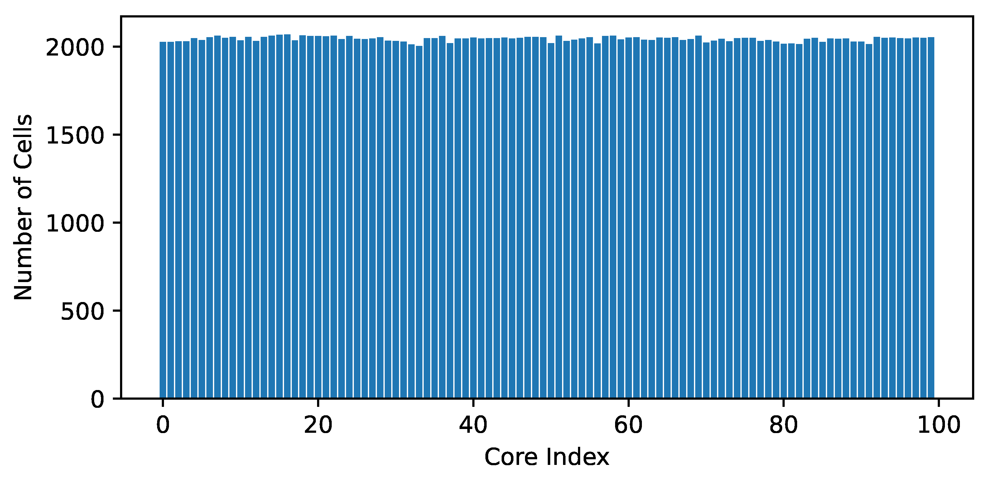
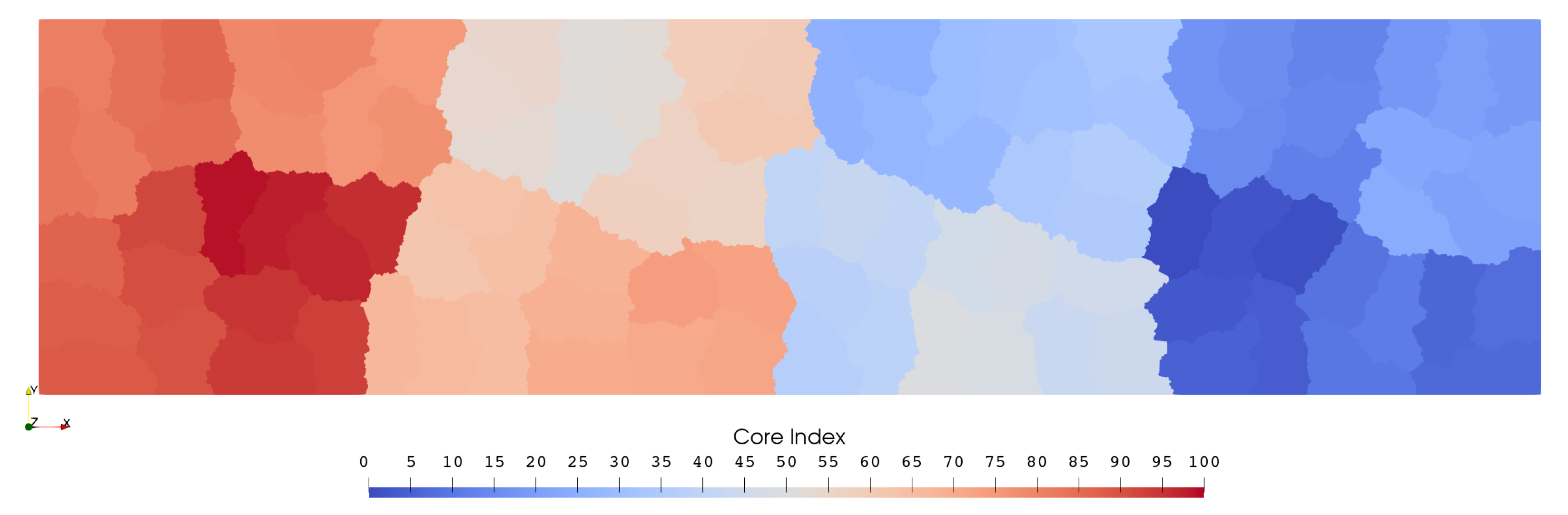
2.4. Parallel Programming

Both the flux integrals (Equation (5)) in the DG method and the function borrowing (Equation (6)) in WENO limiters put a requirement on each cell to access its neighbors in $𝒪$ (1) time, which is not supported by commonly used mesh formats. For this reason, we do not partition the input mesh directly using the METIS_PartMeshDual(...) function as in traditional finite element methods, but convert the mesh to its dual graph by the METIS_MeshToDual(...) function, and then partition the graph using the METIS_PartGraphKway(...) function. The METIS_MeshToDual(...) function stores the cell adjacency information in dynamically allocated arrays pointed by raw pointers, which should then be the released exactly once by some caller in the call stack. To avoid memory bugs, we suggest to wrap such raw pointers into some smart pointers, such as those provided by the standard library of modern C++ [35].

Once we obtain the partitioning, each part of the mesh should then be load by a process, which holds and updates local data sequentially and shares data on inter-part boundaries with neighbors when necessary. This is a typical scenario of the distributed memory parallelization, which achieves acceleration by solving relatively equal-sized subproblems simultaneously on multiple cores. Compared with this, the shared memory parallelization, which provides a global memory address space shared by multiple threads, is generally easier to program but less scalable. The price we paid for scalability is the explicit management of message passing for sharing data between processes. Thanks to the publicly available implementations of the MPI standard, such as MPICH (https://www.mpich.org) and Open-MPI (https://www.open-mpi.org),  the code for doing this is much simpler than it used to be. To improve readability and maintainability of our code, we wrap these communication operations in functions names as ShareSomething(...), which share the same code structure:

• For each destination, put the data to be sent into a sending buffer and register a request of sending by calling the MPI_Isend(...) function.
• For each source, allocate a receiving buffer for the data to be received and register a request of receiving by calling the MPI_Irecv(...) function.
• Performed other computations that can be conducted without communications.
• Block the process until all its requests complete by calling the the MPI_Waitall(...) function.

The third step is optional but may help to improve parallel efficiency, since it allows computations to overlap with communications.

3. Results

In this section, we give the results of various numerical experiments to show the accuracy and performance of the methods described in Section 2. Even though all these experiments can be carried out on one- or two-dimensional structured meshes, we intentionally solve them on three-dimensional unstructured meshes. In this way, the applicability of our solvers for real engineering problems could be demonstrated.

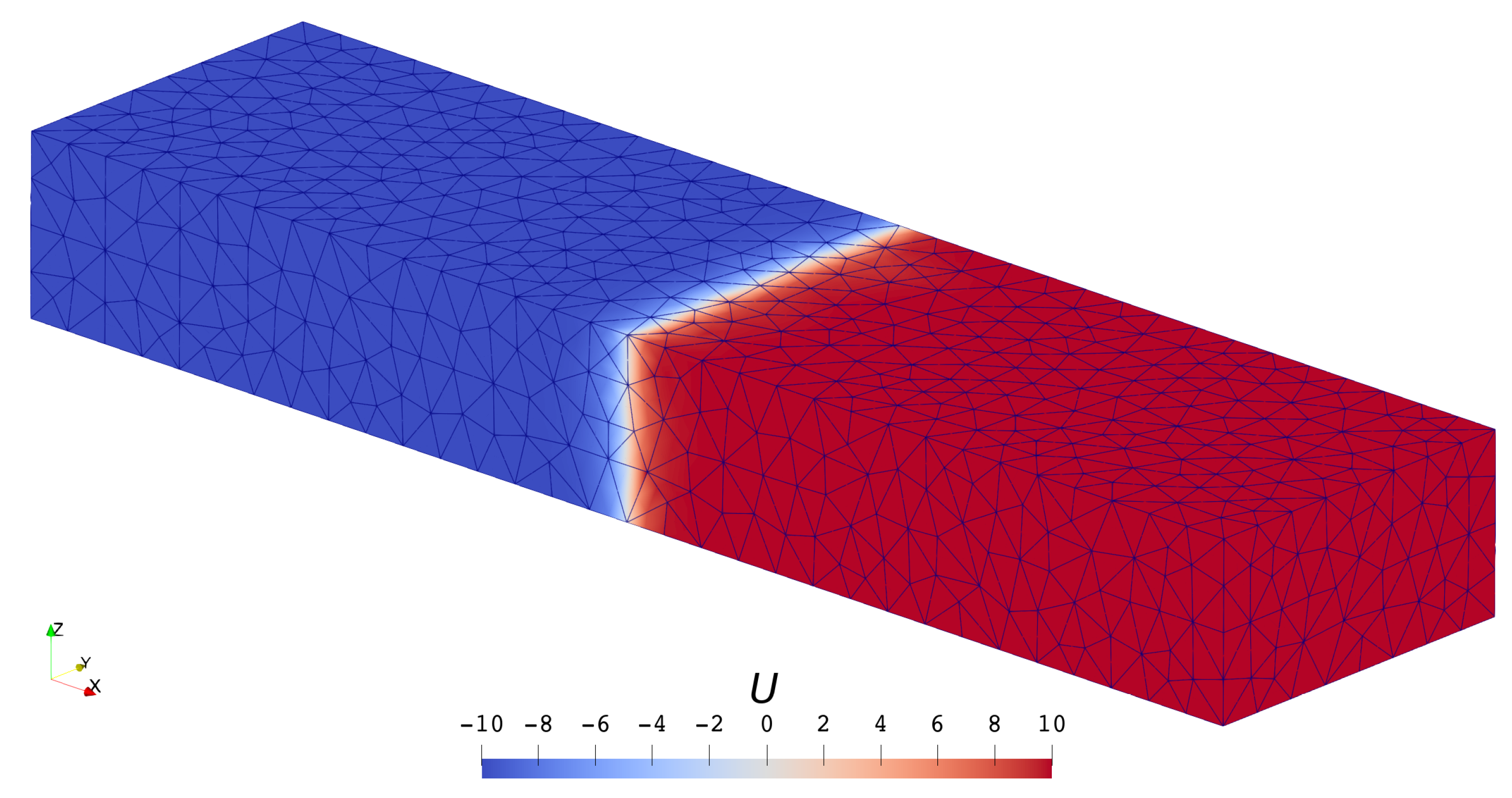
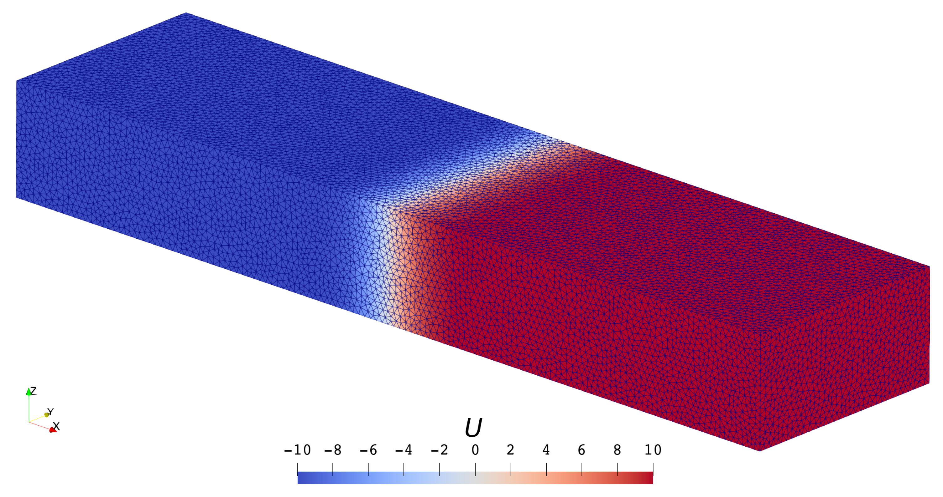
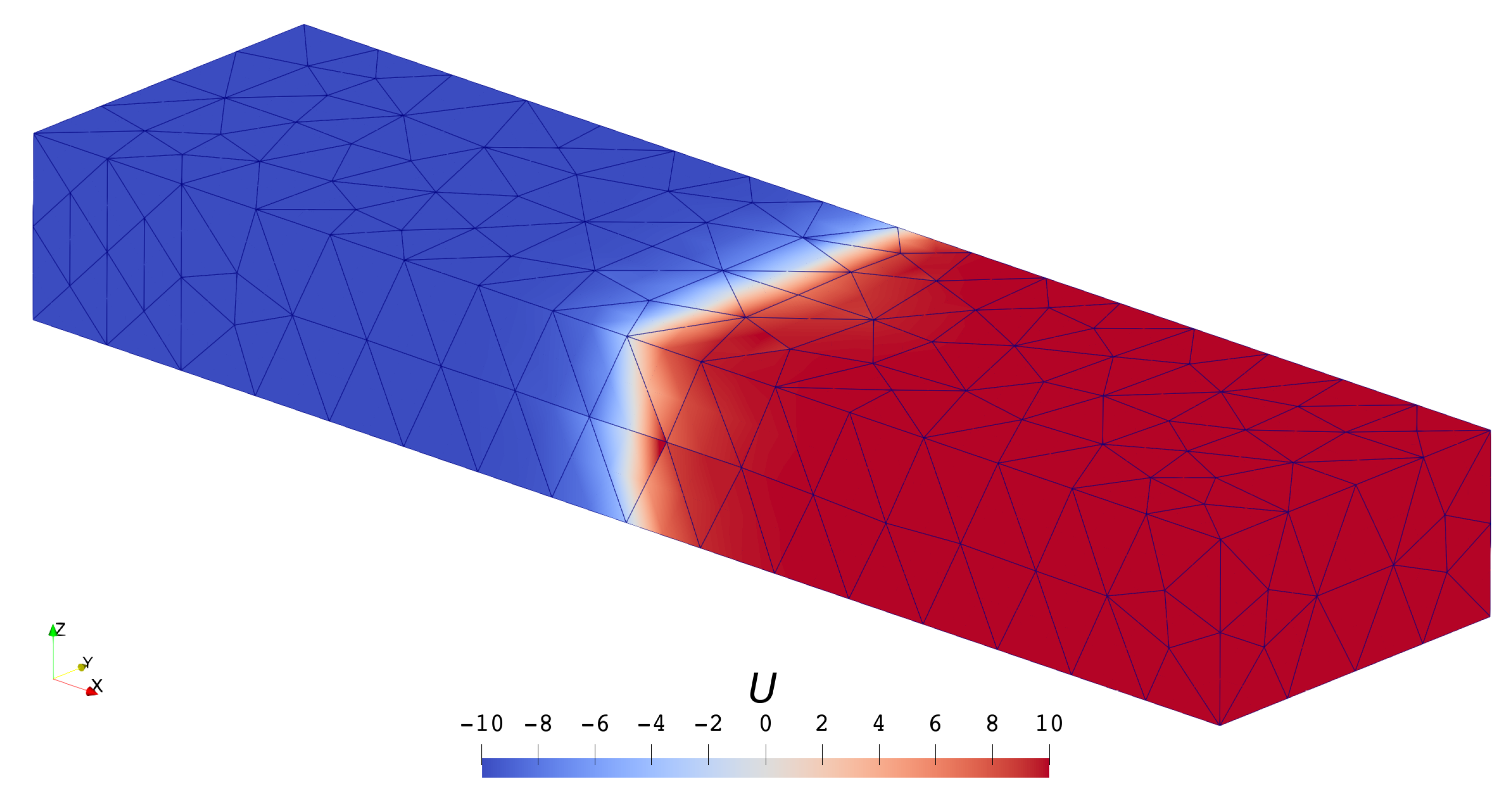
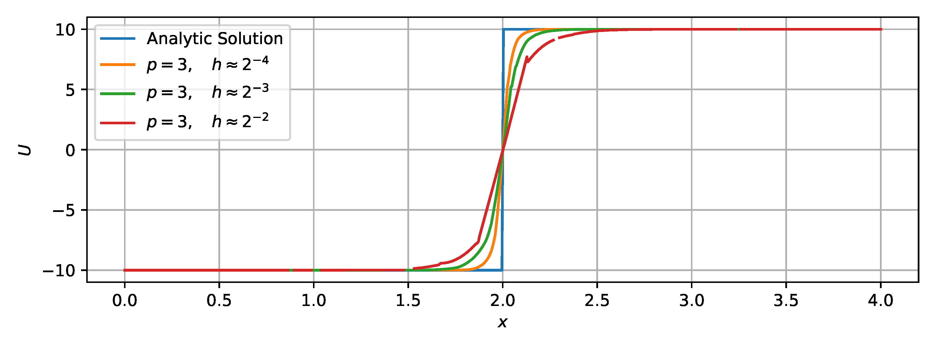
3.1. Linear Conservation Laws

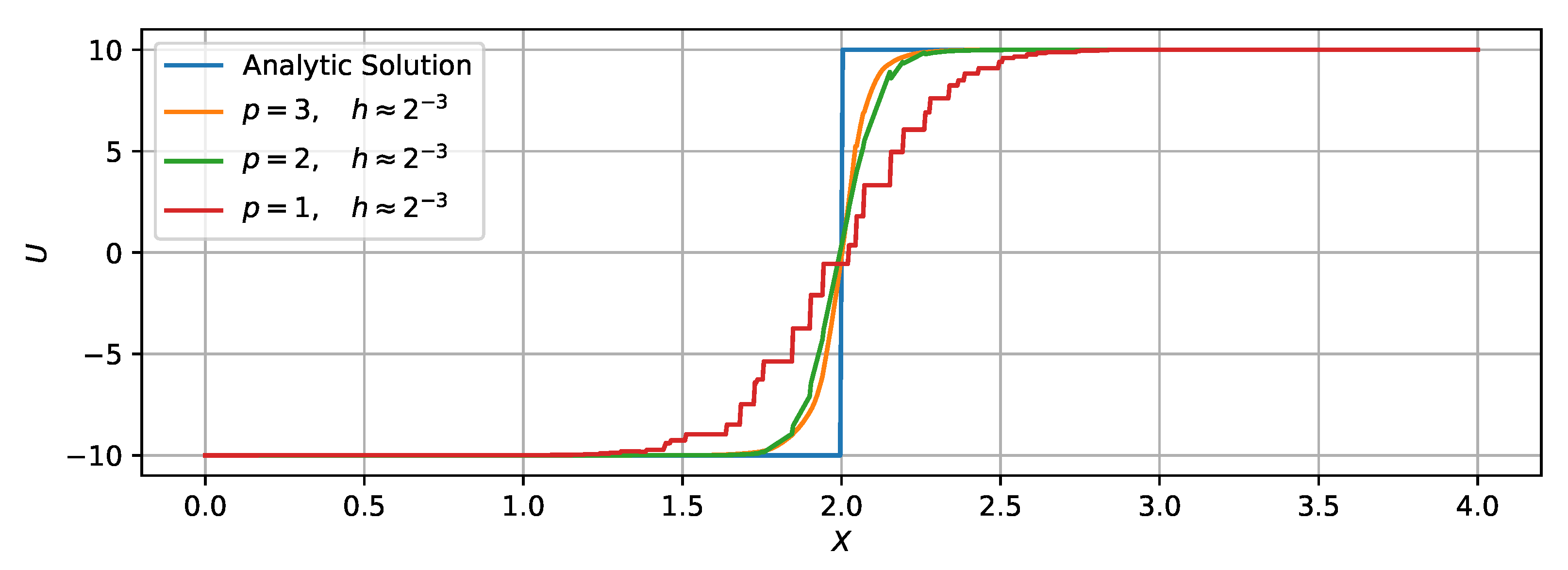
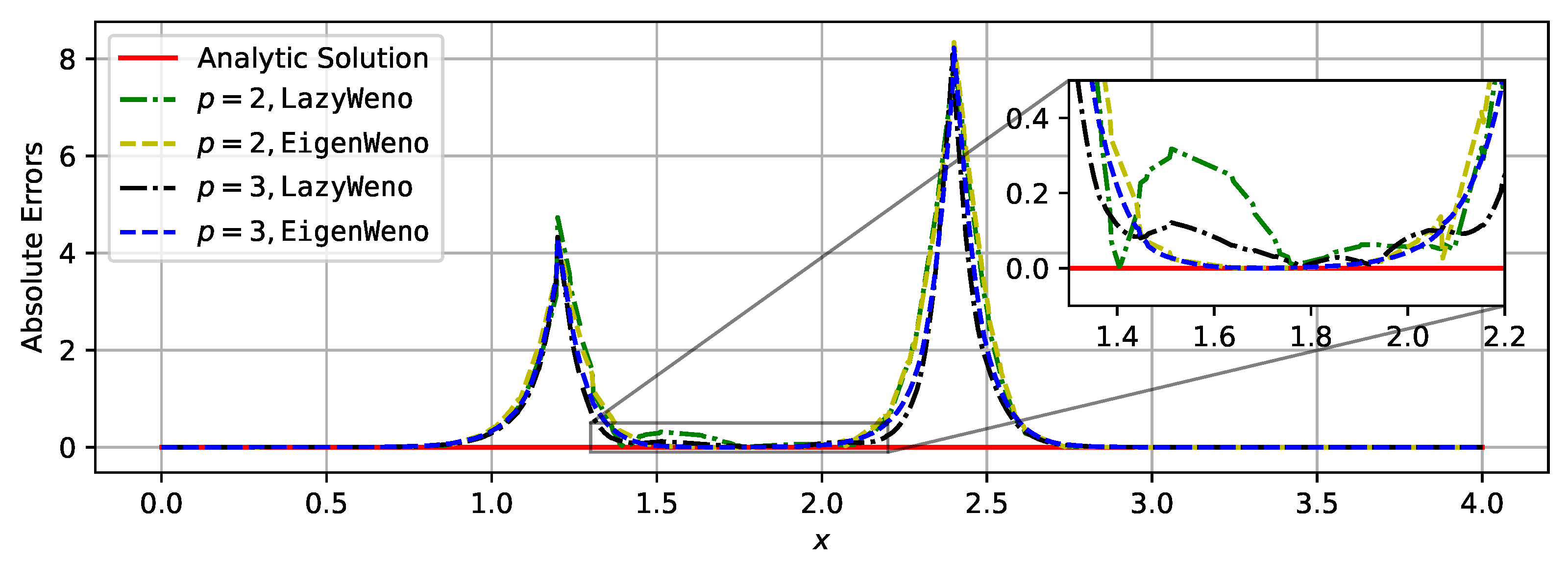
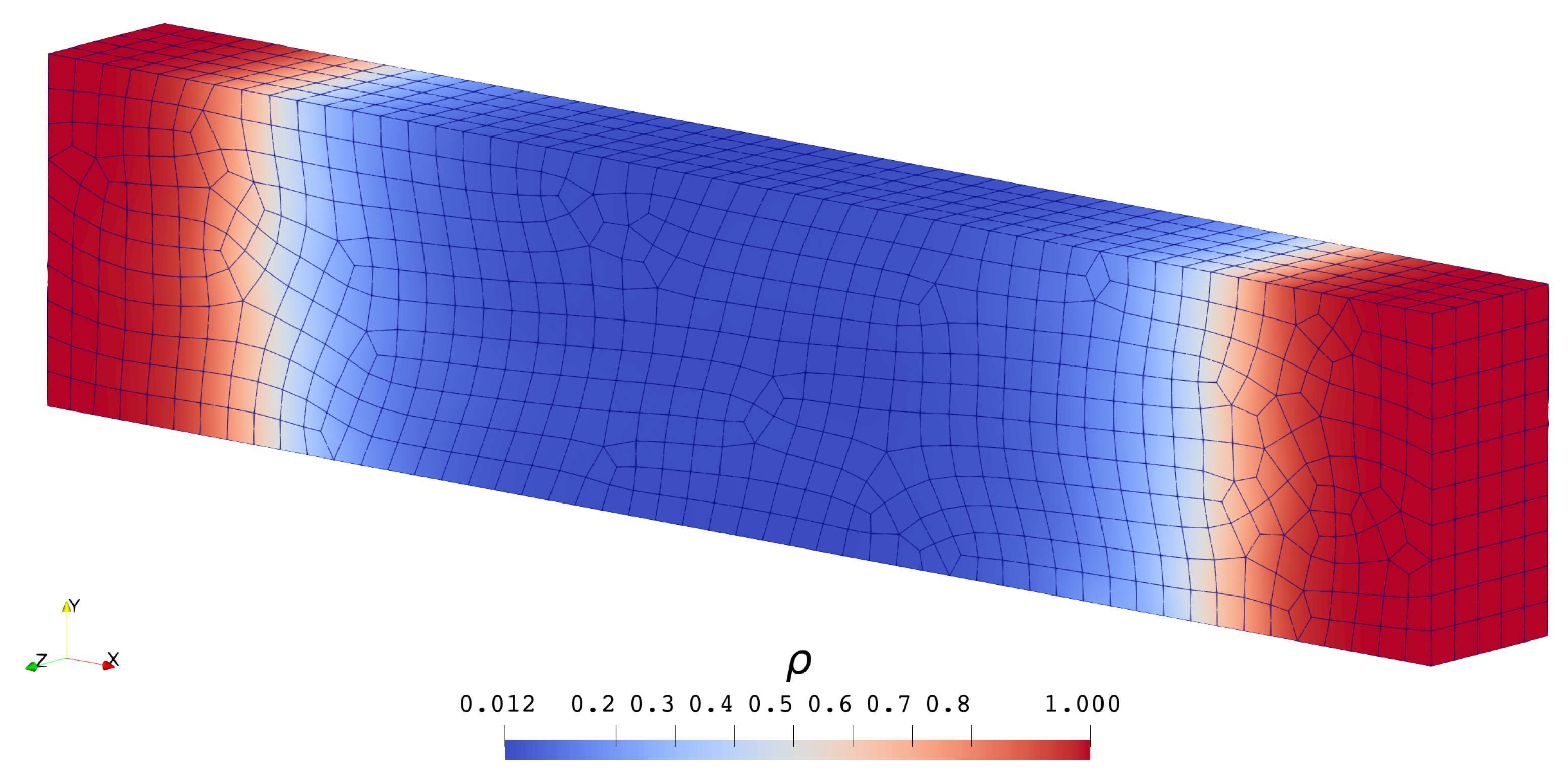
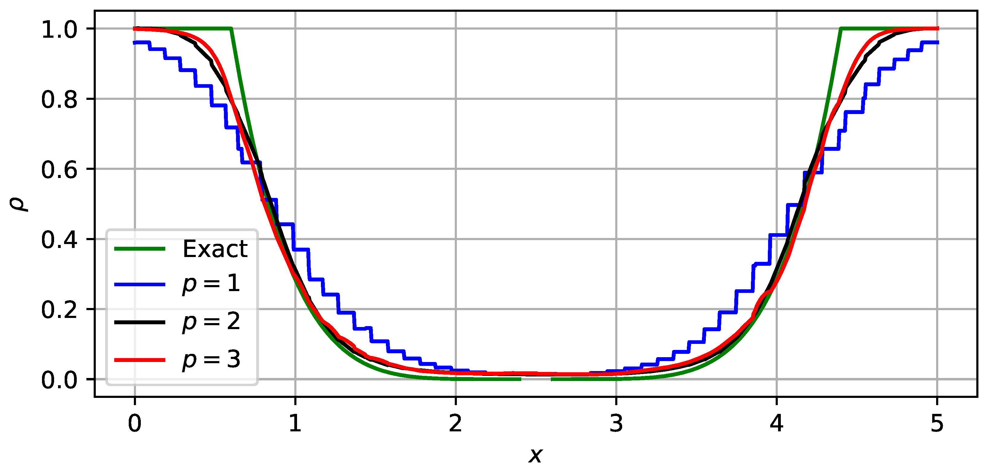
The first group of problems to be solved is the linear version of Equation (1):

$${\partial }_t\underline{U}+\underline{A^x}{\partial }_x\underline{U}+\underline{A^y}{\partial }_y\underline{U}+\underline{A^z}{\partial }_z\underline{U}=\underline{O}$$

(19)

with certain boundary and initial conditions. These problems are mathematically simple in the sense that they can be solved analytically. The existence of analytic solutions gives us a good way to measure the accuracy of our numerical solvers. In this subsection, we use tetrahedral meshes generated in a $[0,4]\times [0,1]\times [0,0.5]$ box.

3.1.1. Scalar Case

This is the simplest case of Equation (19):

Problem 1.

In Equation (19), let $\underline{U}$ consists only one component and each $\underline{A}$ consists a single number:

$$\underline{U}(\overrightarrow{x},t)=\left[\begin{array}{c}U(x,y,z,t)\end{array}\right],\underline{A^x}=\left[\begin{array}{c}-10\end{array}\right],\underline{A^y}=\underline{A^z}=\left[\begin{array}{c}0\end{array}\right].$$

The following boundary conditions

$$\underline{U}(x=0,y,z,t)=\left[\begin{array}{c}-10\end{array}\right]=:{\underline{U}}_{\mathrm{L}},\underline{U}(x=4,y,z,t)=\left[\begin{array}{c}+10\end{array}\right]=:{\underline{U}}_{\mathrm{R}},$$

and the initial condition

$$\underline{U}(x,y,z,t=0)={\underline{U}}_{\mathrm{L}}$$

are applied.

The analytic solution of Problem 1 is:

$$\underline{U}(x,y,z,t)=\left\{\begin{array}{cc}{\underline{U}}_{\mathrm{L}}\hfill & x-4<-10t\hfill \\ {\underline{U}}_{\mathrm{R}}\hfill & x-4>-10t\hfill \end{array}\right.$$

which can be interpreted as a left-running plane wave, whose profile is a jump initially positioned at the right end ($x=4$). To compare the accuracy of various schemes, we plot the meshes and the numerical solutions at the same moment ($t=0.2$) in Figure 1, Figure 2, Figure 3 and Figure 4. The white-colored regions in these figures are continuous transition layers, which are inevitable due to the dissipation of numerical schemes. The thickness of such transition layer, however, can then be used as an indicator of the scheme’s accuracy. Ideally, the thickness should be infinitesimal, as in the analytic solution. The differences between these results are more obvious in Figure 5 and Figure 6, in which we plot the values on 1001 uniformly distributed sample points along the longitudinal axis (on which $y=0.5$ and $z=0.25$) for each solver.

In

Table 1. Accuracy and time cost of each solver–mesh (p–h) pair.

${\mathit{L}}_1$-Error with Respect to the Analytic Solution
	$\mathit{h}$	${\mathbf{2}}^{-\mathbf{2}}$	${\mathbf{2}}^{-\mathbf{3}}$	${\mathbf{2}}^{-\mathbf{4}}$	${\mathbf{2}}^{-\mathbf{5}}$
$\mathit{p}$
1		2.858	2.095	1.524	1.108
2		1.258	0.771	0.463	0.275
3		1.021	0.590	0.341
Time Cost (in Seconds) Measured on a Single Core Whose Main Frequency Is 2.7 GHz
	$\mathit{h}$	${\mathbf{2}}^{-\mathbf{2}}$	${\mathbf{2}}^{-\mathbf{3}}$	${\mathbf{2}}^{-\mathbf{4}}$	${\mathbf{2}}^{-\mathbf{5}}$
$\mathit{p}$
1		0.373	1.129	16.533	306.293
2		1.580	14.894	253.821	4986.391
3		4.147	61.425	906.914

, we show the measured error and time cost of each solver/mesh pair. The seconds consumed by first-order solutions are somewhat exaggerated, since we use the same high-order quadrature rules for both first- and third-order solvers, which is necessary to integrate non-constant errors. If we did not have to measure the errors, then low-order numerical integrators could be used, which might save some time.

The following conclusions can be drawn from both Figure 1, Figure 2, Figure 3, Figure 4, Figure 5 and Figure 6 and Table 1:

• Both mesh refinement (decreasing h) and order increment (increasing p) can help to improve accuracy.
• The solver of the highest order ($p=3$) on the coarsest ($h\approx 2^{-2}$) mesh defeats the solver of the lowest order ($p=1$) on the finest ($h\approx 2^{-5}$) mesh in accuracy but saves quite a lot of time.
• High-order schemes are better than low-order ones in the sense of getting the same level of accuracy with less time cost.

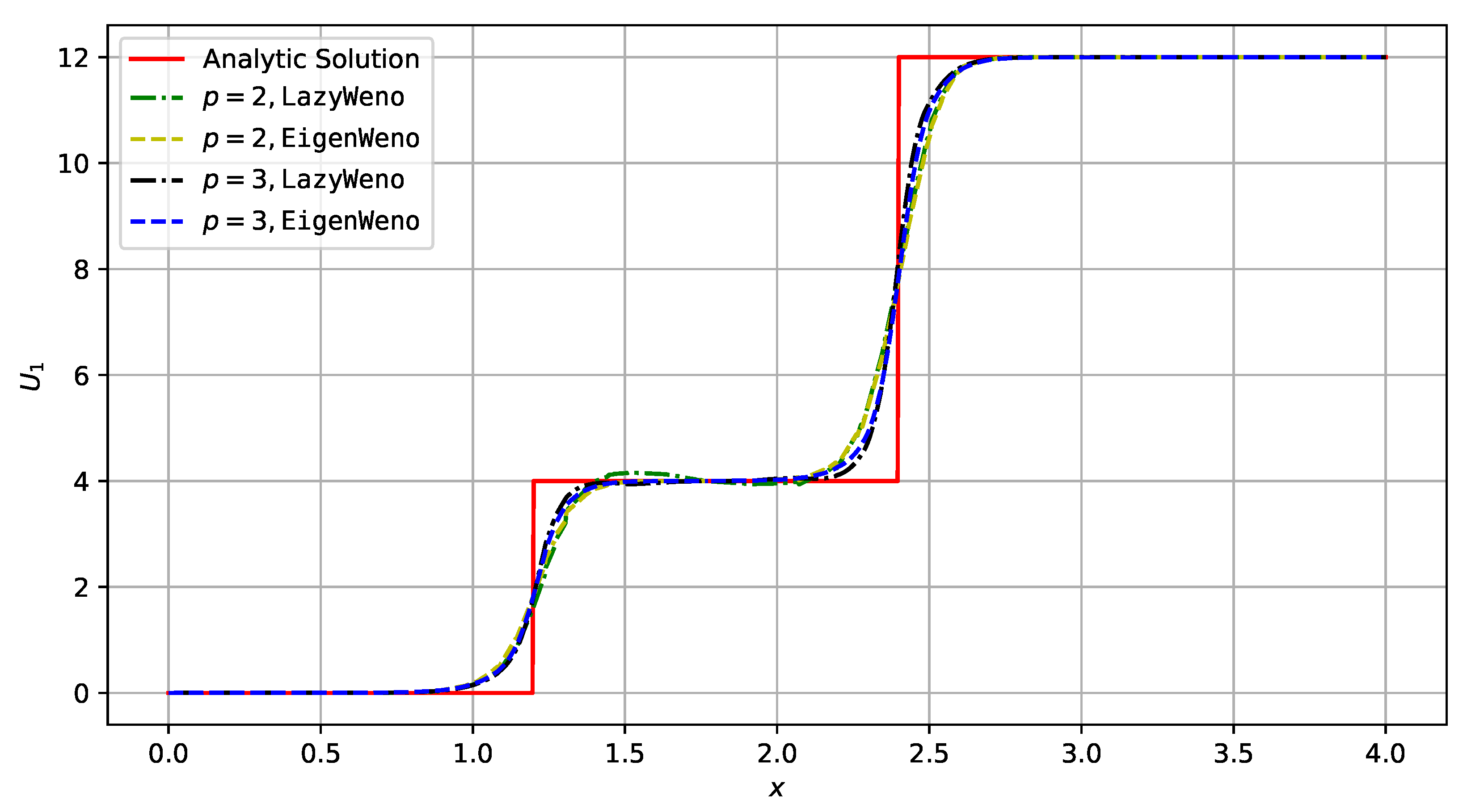
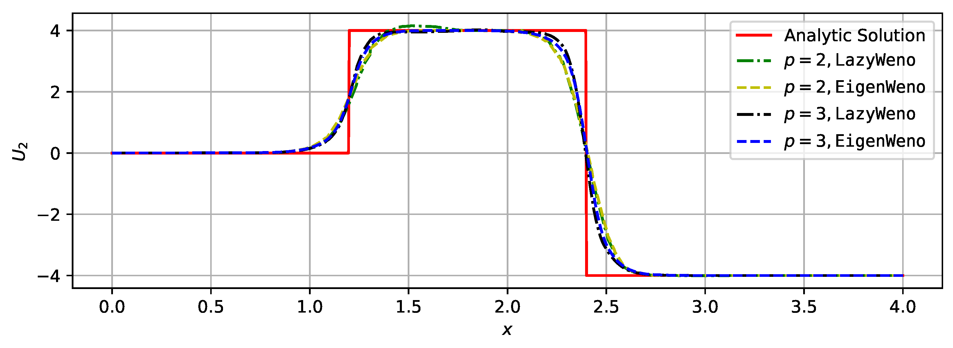
3.1.2. System Case

Problem 2.

In Equation (19), let $\underline{U}$ consists two components and each $\underline{A}$ be a $2\times 2$ matrix:

$$\underline{U}(\overrightarrow{x},t)=\left[\begin{array}{c}{U}_1(x,y,z,t)\\ U_2(x,y,z,t)\end{array}\right],\underline{A^x}=\left[\begin{array}{cc}6& -2\\ -2& 6\end{array}\right],\underline{A^y}=\underline{A^z}=\left[\begin{array}{cc}0& 0\\ 0& 0\end{array}\right],$$

The following boundary conditions

$$\underline{U}(x=0,y,z,t)=\left[\begin{array}{c}0\\ 0\end{array}\right]=:{\underline{U}}_{\mathrm{L}},\underline{U}(x=4,y,z,t)=\left[\begin{array}{c}12\\ -4\end{array}\right]=:{\underline{U}}_{\mathrm{R}},$$

and the initial condition

$$\underline{U}(x,y,z,t=0)={\underline{U}}_{\mathrm{R}}$$

are applied.

To solve this problem analytically, we first obtain the eigenvalue decomposition of $\underline{A^x}$, which is

$$\underset{\underline{A^x}}{\underbrace{\left[\begin{array}{cc}6& -2\\ -2& 6\end{array}\right]}}=\underset{\underline{R^x}}{\underbrace{\left[\begin{array}{cc}1& 1\\ -1& 1\end{array}\right]}}\underset{\underline{{\Lambda }^x}}{\underbrace{\left[\begin{array}{c}8\\ & 4\end{array}\right]}}\underset{{\left(\underline{R^x}\right)}^{-1}}{\underbrace{\left[\begin{array}{cc}1/2& -1/2\\ 1/2& 1/2\end{array}\right]}}$$

By introducing the characteristic variable $\underline{V}:={\left(\underline{R^x}\right)}^{-1}\underline{U}$, which means

$$\left[\begin{array}{c}{V}_1\\ V_2\end{array}\right]:=\left[\begin{array}{cc}1/2& -1/2\\ 1/2& 1/2\end{array}\right]\left[\begin{array}{c}{U}_1\\ U_2\end{array}\right]=\frac{1}{2}\left[\begin{array}{c}{U}_1-U_2\\ U_1+U_2\end{array}\right],$$

the boundary conditions become

$${\underline{V}}_{\mathrm{L}}={\left(\underline{R^x}\right)}^{-1}{\underline{U}}_{\mathrm{L}}=\left[\begin{array}{c}0\\ 0\end{array}\right],{\underline{V}}_{\mathrm{R}}={\left(\underline{R^x}\right)}^{-1}{\underline{U}}_{\mathrm{R}}=\left[\begin{array}{c}8\\ 4\end{array}\right],$$

and the system can be decoupled:

$$\left[\begin{array}{c}{\partial }_t+8{\partial }_x\\ & {\partial }_t+4{\partial }_x\end{array}\right]\left[\begin{array}{c}{V}_1\\ V_2\end{array}\right]=\left[\begin{array}{c}0\\ 0\end{array}\right].$$

We can then solve these two scalar problems independently, which gives

$$V_1(x,y,z,t)=\left\{\begin{array}{cc}0\hfill & x<8t\hfill \\ 8\hfill & x>8t\hfill \end{array}\right.,V_2(x,y,z,t)=\left\{\begin{array}{cc}0\hfill & x<4t\hfill \\ 4\hfill & x>4t\hfill \end{array}\right..$$

The solution of Problem 2 can be obtained by $\underline{U}=\underline{R^x}\underline{V}$, which gives

$$\underline{U}(\overrightarrow{x},t)=\left[\begin{array}{c}{V}_2+V_1\\ V_2-V_1\end{array}\right]=\left\{\begin{array}{cc}{\underline{U}}_{\mathrm{L}}\hfill & x/t<4\hfill \\ {\underline{U}}_{\mathrm{M}}\hfill & x/t\in (4,8)\hfill \\ {\underline{U}}_{\mathrm{R}}\hfill & x/t>8\hfill \end{array}\right.,$$

(20)

where

$${\underline{U}}_{\mathrm{L}}=\left[\begin{array}{c}0\\ 0\end{array}\right],{\underline{U}}_{\mathrm{M}}=\left[\begin{array}{c}4\\ 4\end{array}\right],{\underline{U}}_{\mathrm{R}}=\left[\begin{array}{c}12\\ -4\end{array}\right].$$

With this analytic solution, we can evaluate the accuracy of our numerical solvers. Four solver–limiter pairs are tested on the same mesh ($h\approx 2^{-3}$) used in Figure 1.

We plot the contour of $\underline{U}(x,y,z,t=0.3)$ with the underlying mesh in Figure 7 and Figure 8 and compare the results along the longitudinal axis at $t=0.3$ with the analytic solution in Figure 9 and Figure 10. It is clear that both LazyWeno and EigenWeno (see Section 2.2) can essentially suppress non-physical oscillations in each component. Figure 11 shows that higher-order ($p=3$) solvers still outperforms lower-order ($p=2$) solvers in accuracy and the EigenWeno limiter generally works better than its LazyWeno counterpart. For this reason, we will use EigenWeno limiters exclusively in the rest of this section.

3.2. Inviscid Compressible Flows

The second group of problems to be solved is the three-dimensional Euler system:

$${\partial }_t\left[\begin{array}{c}\rho \\ \rho u_x\\ \rho u_y\\ \rho u_z\\ \rho e_0\end{array}\right]+{\partial }_x\left[\begin{array}{c}\rho u_x\\ \rho u_x{u}_x+p\\ \rho u_y{u}_x\\ \rho u_z{u}_x\\ \rho h_0{u}_x\end{array}\right]+{\partial }_y\left[\begin{array}{c}\rho u_y\\ \rho u_x{u}_y\\ \rho u_y{u}_y+p\\ \rho u_z{u}_y\\ \rho h_0{u}_y\end{array}\right]+{\partial }_z\left[\begin{array}{c}\rho u_z\\ \rho u_x{u}_z\\ \rho u_y{u}_z\\ \rho u_z{u}_z+p\\ \rho h_0{u}_z\end{array}\right]=\left[\begin{array}{c}0\\ 0\\ 0\\ 0\\ 0\end{array}\right]$$

(21)

with certain boundary and initial conditions. These problems are genuinely nonlinear which cannot be solved analytically in general. However, their exact or high-order solutions in lower-dimensional spaces are well known in CFD studies, which can still be used to test our three-dimensional solvers.

For this system, the $\underline{A^{\nu }}$ defined in Equation (12) depends on $\underline{U}$, so do the ${\underline{R}}^{-1}$ in Equation (14) and the $\underline{R}$ in Equation (15). Fortunately, these matrices can be explicitly formulated:

$$\underline{R}\left(\underline{U}\right)=\left[\begin{array}{ccccc}1& 1& 0& 0& 1\\ u_x-a{\nu }_x& u_x& {\sigma }_x& {\pi }_x& u_x+a{\nu }_x\\ u_y-a{\nu }_y& u_y& {\sigma }_y& {\pi }_y& u_y+a{\nu }_y\\ u_z-a{\nu }_z& u_z& {\sigma }_z& {\pi }_z& u_z+a{\nu }_z\\ h_0-u_{\nu }a& \frac{u_x^2+u_y^2+u_z^2}{2}& u_{\sigma }& u_{\pi }& h_0+u_{\nu }a\end{array}\right],\left[\begin{array}{c}{u}_{\nu }\\ u_{\sigma }\\ u_{\pi }\end{array}\right]={\left[\begin{array}{ccc}{\nu }_x& {\sigma }_x& {\pi }_x\\ {\nu }_y& {\sigma }_y& {\pi }_y\\ {\nu }_z& {\sigma }_z& {\pi }_z\end{array}\right]}^{-1}\left[\begin{array}{c}{u}_x\\ u_y\\ u_z\end{array}\right],$$

$$\underline{L}\left(\underline{U}\right)=\left[\begin{array}{ccccc}\frac{1}{2}\left(B_2+\frac{u_{\nu }}{a}\right)& \frac{-1}{2}\left(B_1{u}_x+\frac{{\nu }_x}{a}\right)& \frac{-1}{2}\left(B_1{u}_y+\frac{{\nu }_y}{a}\right)& \frac{-1}{2}\left(B_1{u}_z+\frac{{\nu }_z}{a}\right)& \frac{1}{2}{B}_1\\ 1-B_2& B_1{u}_x& B_1{u}_y& B_1{u}_z& -B_1\\ -u_{\sigma }& {\sigma }_x& {\sigma }_y& {\sigma }_z& 0\\ -u_{\pi }& {\pi }_x& {\pi }_y& {\pi }_z& 0\\ \frac{1}{2}\left(B_2-\frac{u_{\nu }}{a}\right)& \frac{-1}{2}\left(B_1{u}_x-\frac{{\nu }_x}{a}\right)& \frac{-1}{2}\left(B_1{u}_y-\frac{{\nu }_y}{a}\right)& \frac{-1}{2}\left(B_1{u}_z-\frac{{\nu }_z}{a}\right)& \frac{1}{2}{B}_1\end{array}\right],$$

in which $B_1:=(\gamma -1)/a^2$ and $B_2:=B_1(u_{\nu }^2+u_{\sigma }^2+u_{\pi }^2)$.

3.2.1. Shock Tube Problems

These problems are usually defined as one-dimensional problems, but we treat them as three-dimensional ones. All these problems are considered in a $[0.0,5.0]\times [0.0,1.0]\times [0.0,0.5]$ box with all boundaries closed but the left and right ends open. Although no analytic solutions exist, we can still use the method described in [31], which solves nonlinear algebraic equations numerically, to obtain their exact solutions. To test the numerical methods described in Section 2, we use the unstructured hexahedral mesh in Figure 12, in which $h\approx 1/10$.

Problem 3

(Sod). Solve the Euler system (Equation (21)) for $t\in [0.0,1.0]$ with the initial condition

$${\left[\begin{array}{ccccc}\rho & u& vs.& w& p\end{array}\right]}_{t=0}=\left\{\begin{array}{cc}\left[\begin{array}{ccccc}1.000& 0.000& 0.000& 0.000& 1.000\end{array}\right]\hfill & x<2\hfill \\ \left[\begin{array}{ccccc}0.125& 0.000& 0.000& 0.000& 0.100\end{array}\right]\hfill & x>2\hfill \end{array}\right.$$

Problem 4

(Lax). Solve the Euler system (Equation (21)) for $t\in [0.0,0.6]$ with the initial condition

$${\left[\begin{array}{ccccc}\rho & u& vs.& w& p\end{array}\right]}_{t=0}=\left\{\begin{array}{cc}\left[\begin{array}{ccccc}0.445& 0.698& 0.000& 0.000& 3.528\end{array}\right]\hfill & x<2\hfill \\ \left[\begin{array}{ccccc}0.500& 0.000& 0.000& 0.000& 0.571\end{array}\right]\hfill & x>2\hfill \end{array}\right.$$

Problem 5

(Vacuum). Solve the Euler system (Equation (21)) for $t\in [0.0,0.3]$ with the initial condition

$${\left[\begin{array}{ccccc}\rho & u& vs.& w& p\end{array}\right]}_{t=0}=\left\{\begin{array}{cc}\left[\begin{array}{ccccc}1.0& -4.0& 0.0& 0.0& 0.4\end{array}\right]\hfill & x<2\hfill \\ \left[\begin{array}{ccccc}1.0& +4.0& 0.0& 0.0& 0.4\end{array}\right]\hfill & x>2\hfill \end{array}\right.$$

In Figure 13, Figure 14 and Figure 15, we plot the density contours given by the same third-order solver with an EigenWeno limiter. In Figure 13, Figure 14, Figure 15, Figure 16, Figure 17 and Figure 18, we plot the density distributions along the longitudinal axis (on which $y=0.5$ and $z=0.25$) of the box. All these results show that higher-order ($p=3$) solvers with EigenWeno limiters are better than lower-order ($p=1$) solvers at capturing discontinuities (shocks, contacts, expansions), which may occur frequently in compressible flows.

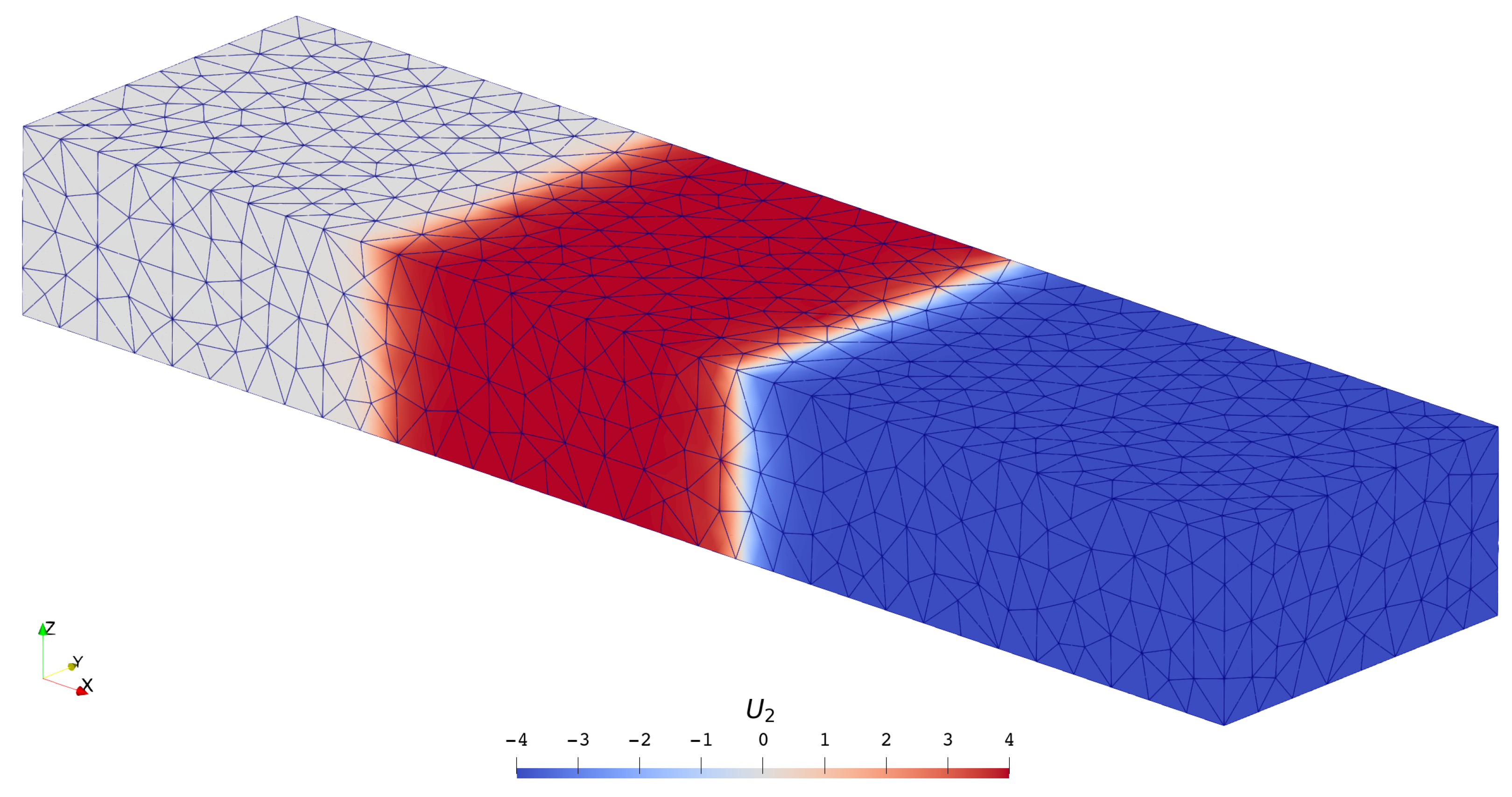
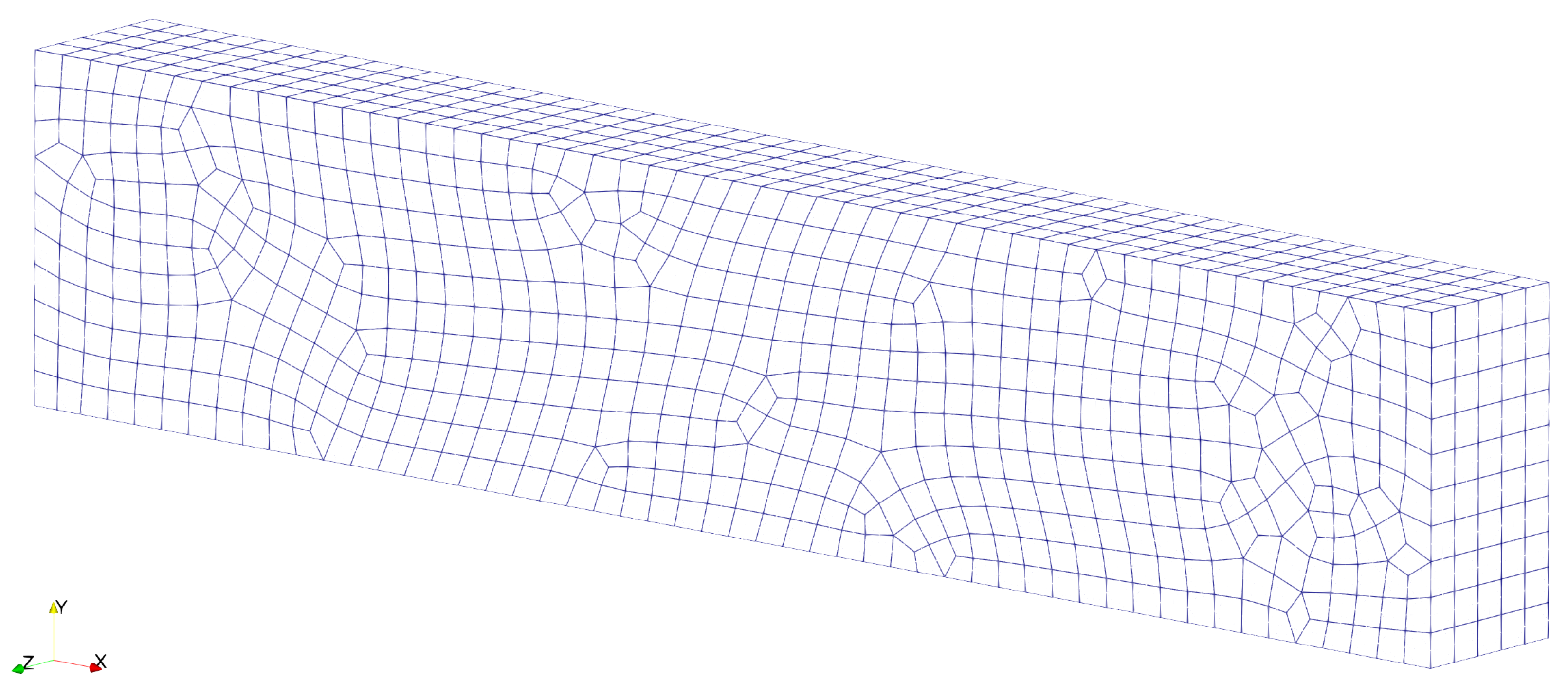
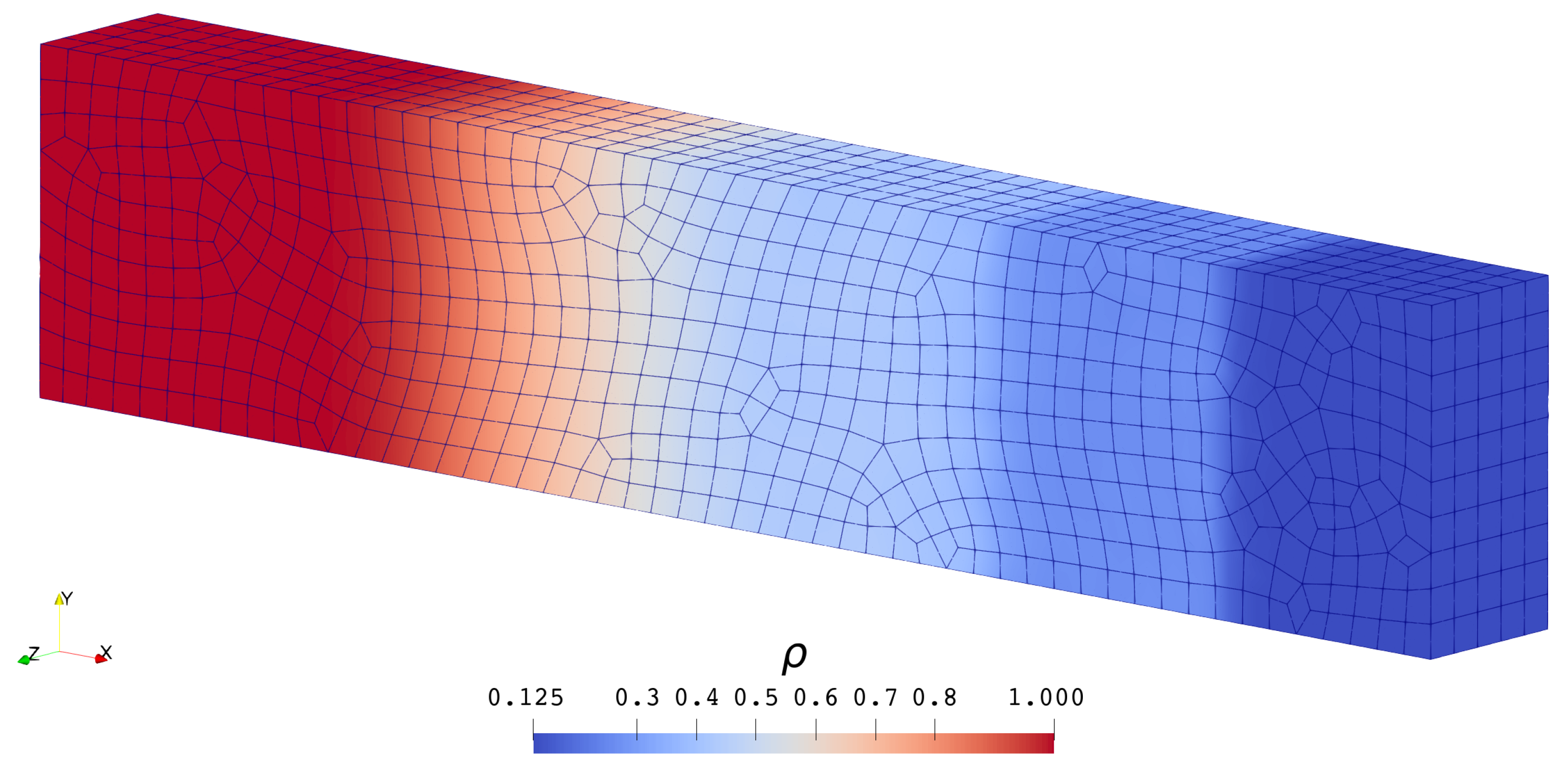
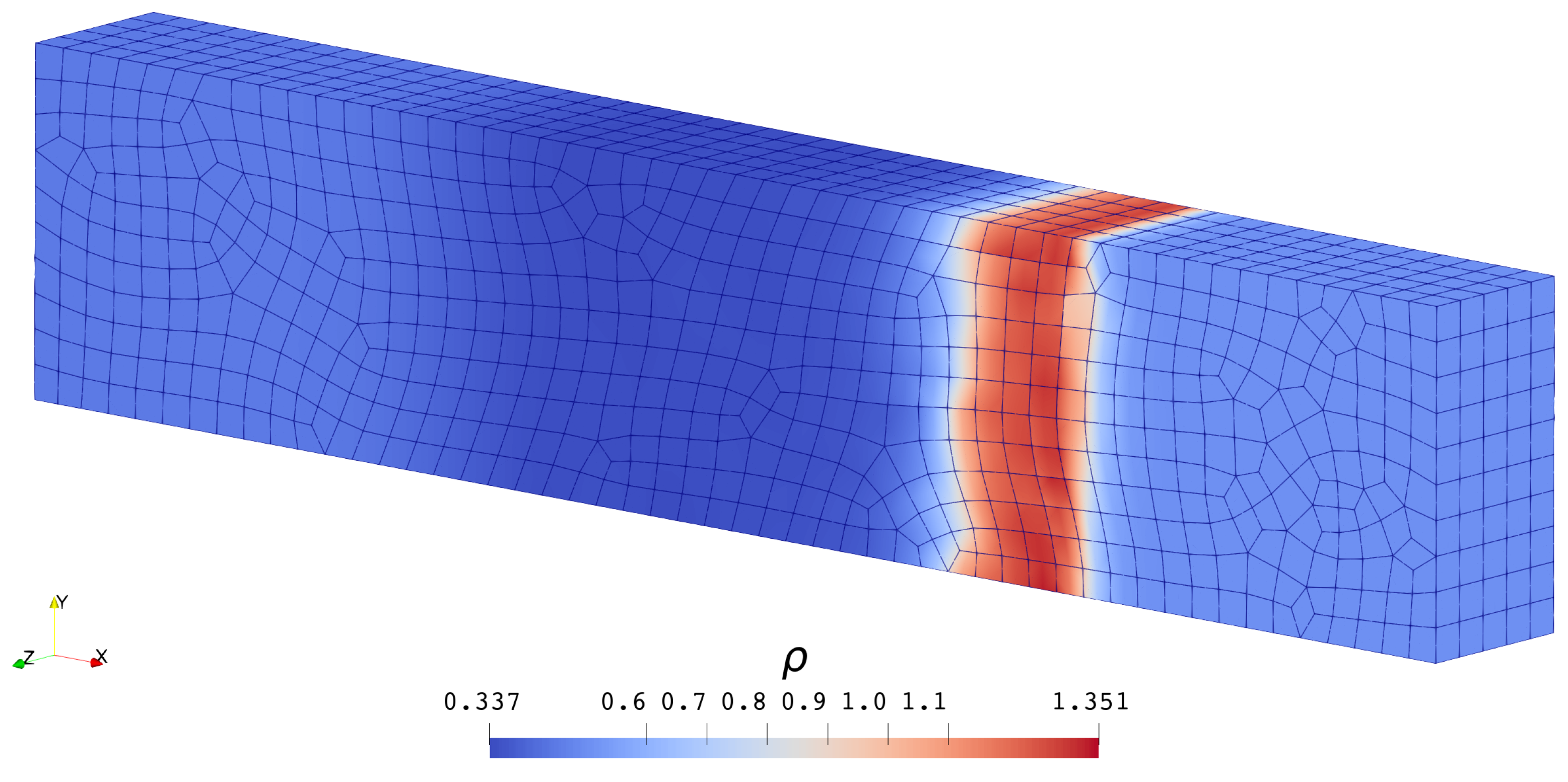
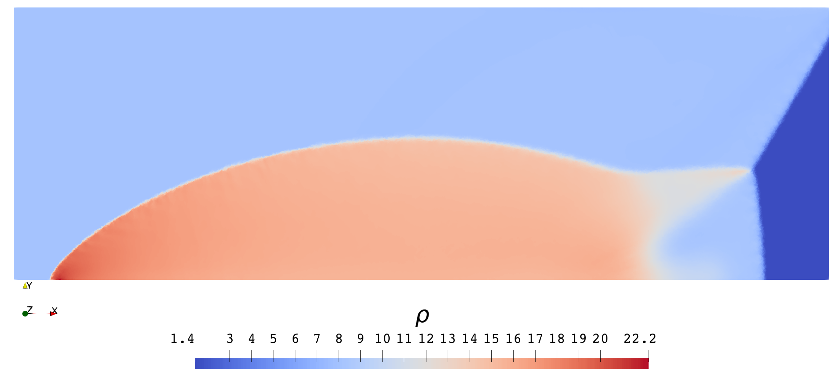
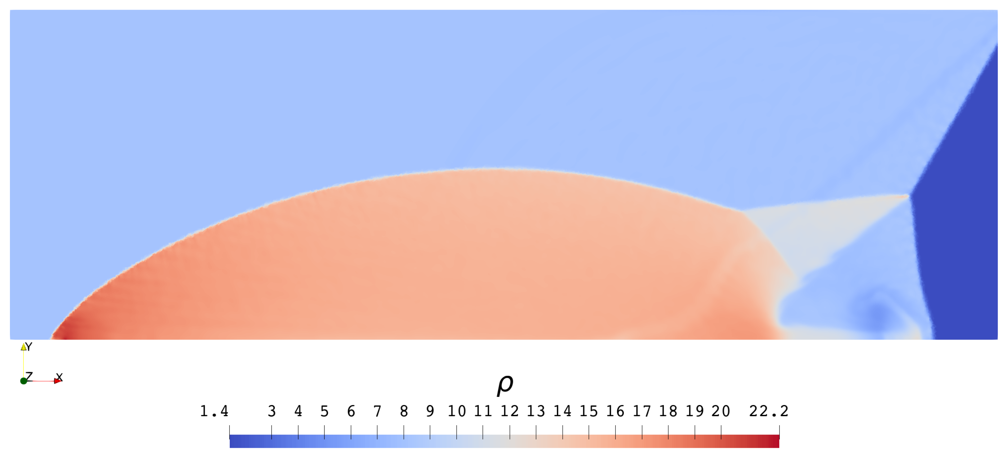
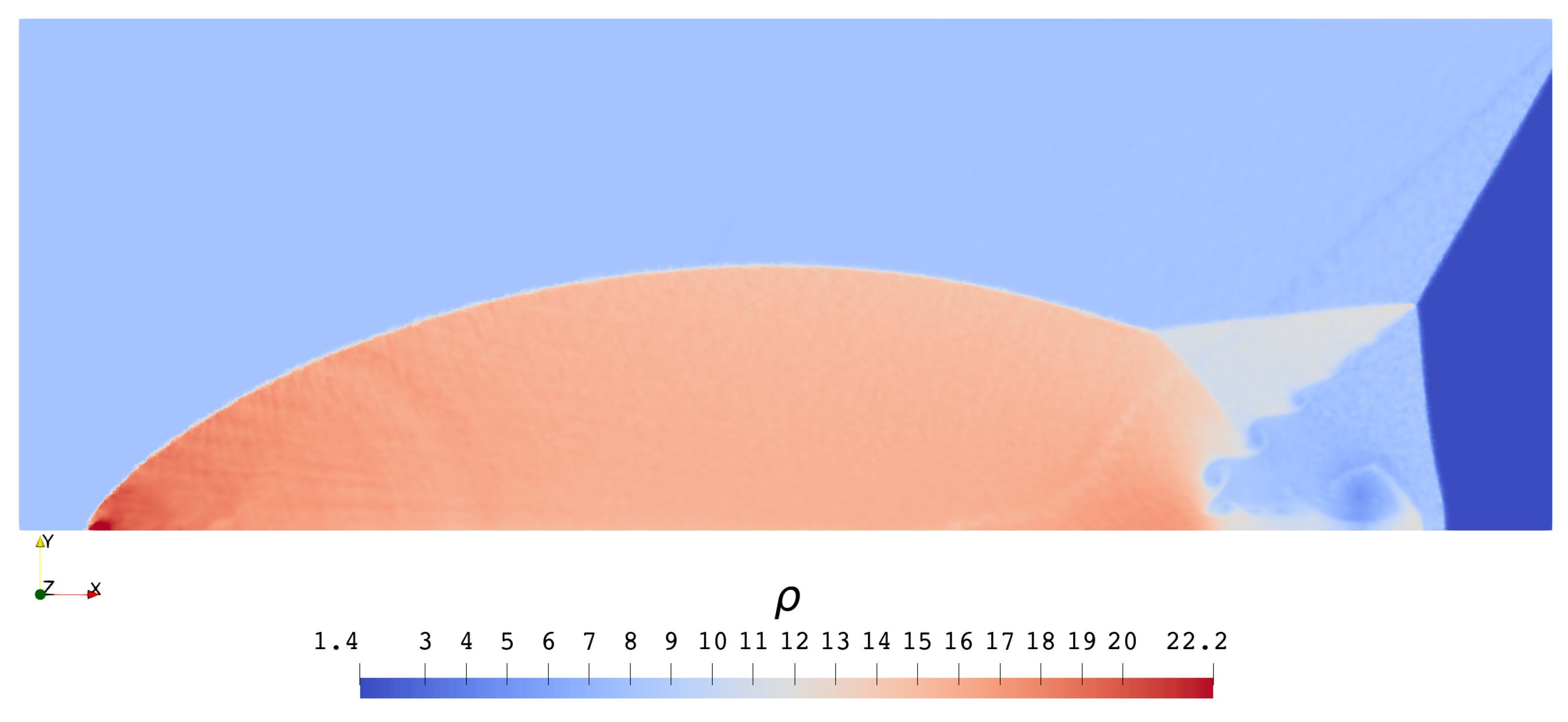
3.2.2. Double Mach Reflection Problem

This is a classical two-dimensional problem originally proposed in [36], which we redefine here as a three-dimensional one:

Problem 6.

Solve the Euler system (Equation (21)) in the region defined in Figure 19, in which $x_0=1/6$. The initial condition is given as a moving shock wave:

$${\left[\begin{array}{ccccc}\rho & u& vs.& w& p\end{array}\right]}_{t=0}=\left\{\begin{array}{cc}\left[\begin{array}{ccccc}1.4& 0.0& 0.0& 0.0& 1.0\end{array}\right]\hfill & y<\sqrt{3}(x-x_0)\hfill \\ \left[\begin{array}{ccccc}8.0& u_{\mathrm{A}}& v_{\mathrm{A}}& 0.0& 116.5\end{array}\right]\hfill & y>\sqrt{3}(x-x_0)\hfill \end{array}\right.,$$

(22)

in which $u_{\mathrm{A}}=4.125\sqrt{3}$ and $v_{\mathrm{A}}=-4.125$ are the velocity components after the shock wave. The boundary conditions are given as following:

• The $x=0$ surface is open as an inlet;
• The $x=4$ surface and the $x<x_0$ part of the $y=0$ surface are open as outlets;
• The $x>x_0$ part of the $y=0$ surface is closed as a solid wall;
• The $y=1$ surface has the following prescribed state:

$$\left[\begin{array}{ccccc}\rho & u& vs.& w& p\end{array}\right]=\left\{\begin{array}{cc}\left[\begin{array}{ccccc}1.4& 0.0& 0.0& 0.0& 1.0\end{array}\right]\hfill & 1<\sqrt{3}(x-(x_0+u_{\mathrm{A}}t))\hfill \\ \left[\begin{array}{ccccc}8.0& u_{\mathrm{A}}& v_{\mathrm{A}}& 0.0& 116.5\end{array}\right]\hfill & 1>\sqrt{3}(x-(x_0+u_{\mathrm{A}}t))\hfill \end{array}\right.,$$

which is consistent with the initial condition (Equation (22)).

As a common practice, we plot the density contour at $t=0.2$ in a $[0,3]\times [0,1]$ rectangle (on the $z=0$ surface) for each solver in Figure 20, Figure 21 and Figure 22. It is clear that as the accuracy order increases, the thickness of each discontinuity decreases and the rolled-up vortex structure becomes more clear.

Before concluding this section, we provide the measured performance of our third-order solver that produces Figure 22 in

Table 2. Performance of the same solver running on different number of cores.

P	${\mathit{T}}_{100}$	${\mathit{T}}_{199}$	${\mathit{T}}_{200}$	$\mathit{P}\frac{{\mathit{T}}_{199}-{\mathit{T}}_{100}}{99}$	$\mathit{P}\frac{{\mathit{T}}_{200}-{\mathit{T}}_{100}}{100}$
1	17,652.2	35,324.5	35,519.3	178.508	178.671
20	960.443	1912.365	1926.584	192.307	193.228
40	491.070	971.710	983.933	194.198	197.145
60	335.651	666.548	676.930	200.544	204.767
80	251.548	494.541	504.951	196.358	202.722
100	202.789	397.641	408.126	196.820	205.337

, in which

• P means the number of processes (one process per core).
• $T_n$ means the wall clock time to finish the first n step.
• $P\frac{T_{m+m}-T_n}{m}$ is the core time per step. The total core time of all steps is often used as an index for charging by high performance computing centers.

Since parallel I/O operations require many collective communications, we write one frame every 100 steps. Thus, the difference between the values in the last two columns is the amortized core time of writing per step. We have to admit that this cost is growing as the number of cores increases. If the number of cores keeps increasing, this may be a bottleneck of maintaining scalability.

The community of parallel computing usually use the speedup (S) and efficiency (E) defined as

$$S=\frac{T_{\mathrm{serial}}}{T_{\mathrm{parallel}}},E=\frac{S}{P}\times 100\%,$$

to assess the performance a parallel program. We follow this practice, calculate these values based on the measured data given in Table 2 and plot them in Figure 23 and Figure 24. These figures show again that the I/O operations have adverse effects on the parallel performance.

The efficiency values given in Figure 24 fluctuate around $90\%$, which are not as good as those above $99\%$ in [26]. One source of such gap is the imperfect load balancing of our tests. Since we are using a three-dimensional unstructured mesh, it can hardly be partitioned uniformly, which is an $NP$-hard problem. On the other hand, their meshes are one- and two-dimensional structured, on which uniform partitioning can be trivially achieved. Figure 25 gives the distribution of cells of the 100-part mesh partitioning (Figure 26) used in this section, which shows a $3\%$ fluctuation.

4. Discussion

In this article, we have formulated the RKDG methods and the WENO limiters for three-dimensional unstructured meshes. The algorithms have been implemented on top of the MPI standard, which supports distributed memory parallelization. The numerical experiments have shown that increasing a solver’s accuracy order helps more to produce better results than just refining the mesh it uses. The efficient parallel implementation has made the time cost affordable for large problems, as long as the solvers can be executed on sufficiently large number of cores. Extending the methods to Navier–Stokes equations and applications of these high-order parallel solvers to real engineering problems are ongoing works. Further optimization of the parallel I/O module may be conducted to achieve better parallel performance.

References

1. Hesthaven, J.S.; Warburton, T. Nodal Discontinuous Galerkin Methods; Springer: New York, NY, USA, 2008. [Google Scholar] [CrossRef] [Green Version]
2. Reed, W.H.; Hill, T.R. Triangular Mesh Methods for the Neutron Transport Equation; Technical Report LA-UR-73-479; Los Alamos Scientific Lab.: Los Alamos, NM, USA, 1973. [Google Scholar]
3. Chavent, G.; Salzano, G. A finite-element method for the 1-D water flooding problem with gravity. J. Comput. Phys. 1982, 45, 307–344. [Google Scholar] [CrossRef]
4. Cockburn, B.; Shu, C.W. The Runge-Kutta local projection P1-discontinuous-Galerkin finite element method for scalar conservation laws. In Proceedings of the 1st National Fluid Dynamics Conference, Cincinnati, OH, USA, 25–28 July 1988; American Institute of Aeronautics and Astronautics: Reston, VA, USA, 1988. [Google Scholar] [CrossRef] [Green Version]
5. Shu, C.W.; Osher, S. Efficient implementation of essentially non-oscillatory shock-capturing schemes. J. Comput. Phys. 1988, 77, 439–471. [Google Scholar] [CrossRef] [Green Version]
6. Shu, C.W.; Osher, S. Efficient implementation of essentially non-oscillatory shock-capturing schemes, II. J. Comput. Phys. 1989, 83, 32–78. [Google Scholar] [CrossRef]
7. Cockburn, B.; Lin, S.Y.; Shu, C.W. TVB Runge-Kutta local projection discontinuous Galerkin finite element method for conservation laws III: One-dimensional systems. J. Comput. Phys. 1989, 84, 90–113. [Google Scholar] [CrossRef] [Green Version]
8. Cockburn, B.; Hou, S.; Shu, C.W. The Runge-Kutta local projection discontinuous Galerkin finite element method for conservation laws. IV. The multidimensional case. Math. Comput. 1990, 54, 545–581. [Google Scholar] [CrossRef] [Green Version]
9. Cockburn, B. An introduction to the Discontinuous Galerkin method for convection-dominated problems. In Lecture Notes in Mathematics; Springer: Berlin/Heidelberg, Germany, 1998; pp. 150–268. [Google Scholar] [CrossRef]
10. Bassi, F.; Rebay, S. A High-Order Accurate Discontinuous Finite Element Method for the Numerical Solution of the Compressible Navier–Stokes Equations. J. Comput. Phys. 1997, 131, 267–279. [Google Scholar] [CrossRef]
11. Cockburn, B.; Shu, C.W. The Local Discontinuous Galerkin Method for Time-Dependent Convection-Diffusion Systems. SIAM J. Numer. Anal. 1998, 35, 2440–2463. [Google Scholar] [CrossRef]
12. Cockburn, B.; Shu, C.W. Runge–Kutta Discontinuous Galerkin Methods for Convection-Dominated Problems. J. Sci. Comput. 2001, 16, 173–261. [Google Scholar] [CrossRef]
13. Gottlieb, D.; Shu, C.W. On the Gibbs Phenomenon and Its Resolution. SIAM Rev. 1997, 39, 644–668. [Google Scholar] [CrossRef] [Green Version]
14. Leer, B.V. Towards the ultimate conservative difference scheme III. Upstream-centered finite-difference schemes for ideal compressible flow. J. Comput. Phys. 1977, 23, 263–275. [Google Scholar] [CrossRef]
15. Leer, B.V. Towards the ultimate conservative difference scheme. IV. A new approach to numerical convection. J. Comput. Phys. 1977, 23, 276–299. [Google Scholar] [CrossRef]
16. van Leer, B. Towards the ultimate conservative difference scheme. V. A second-order sequel to Godunov’s method. J. Comput. Phys. 1979, 32, 101–136. [Google Scholar] [CrossRef]
17. van Leer, B.; Nishikawa, H. Towards the ultimate understanding of MUSCL: Pitfalls in achieving third-order accuracy. J. Comput. Phys. 2021, 446, 110640. [Google Scholar] [CrossRef]
18. Harten, A.; Engquist, B.; Osher, S.; Chakravarthy, S.R. Uniformly High Order Accurate Essentially Non-oscillatory Schemes, III. J. Comput. Phys. 1997, 131, 3–47. [Google Scholar] [CrossRef]
19. Jiang, G.S.; Shu, C.W. Efficient Implementation of Weighted ENO Schemes. J. Comput. Phys. 1996, 126, 202–228. [Google Scholar] [CrossRef] [Green Version]
20. Hu, C.; Shu, C.W. Weighted Essentially Non-oscillatory Schemes on Triangular Meshes. J. Comput. Phys. 1999, 150, 97–127. [Google Scholar] [CrossRef] [Green Version]
21. Qiu, J.; Shu, C.W. Runge–Kutta Discontinuous Galerkin Method Using WENO Limiters. SIAM J. Sci. Comput. 2005, 26, 907–929. [Google Scholar] [CrossRef]
22. Zhu, J.; Qiu, J.; Shu, C.W.; Dumbser, M. Runge–Kutta discontinuous Galerkin method using WENO limiters II: Unstructured meshes. J. Comput. Phys. 2008, 227, 4330–4353. [Google Scholar] [CrossRef]
23. Zhong, X.; Shu, C.W. A simple weighted essentially nonoscillatory limiter for Runge–Kutta discontinuous Galerkin methods. J. Comput. Phys. 2013, 232, 397–415. [Google Scholar] [CrossRef]
24. Zhu, J.; Zhong, X.; Shu, C.W.; Qiu, J. Runge–Kutta discontinuous Galerkin method using a new type of WENO limiters on unstructured meshes. J. Comput. Phys. 2013, 248, 200–220. [Google Scholar] [CrossRef]
25. Mazaheri, A.; Shu, C.W.; Perrier, V. Bounded and compact weighted essentially nonoscillatory limiters for discontinuous Galerkin schemes: Triangular elements. J. Comput. Phys. 2019, 395, 461–488. [Google Scholar] [CrossRef]
26. Biswas, R.; Devine, K.D.; Flaherty, J.E. Parallel, adaptive finite element methods for conservation laws. Appl. Numer. Math. 1994, 14, 255–283. [Google Scholar] [CrossRef]
27. Bey, K.S.; Patra, A.; Oden, J.T. hp-version discontinuous Galerkin methods for hyperbolic conservation laws: A parallel adaptive strategy. Int. J. Numer. Methods Eng. 1995, 38, 3889–3908. [Google Scholar] [CrossRef]
28. Chalmers, N.; Agbaglah, G.; Chrust, M.; Mavriplis, C. A parallel hp-adaptive high order discontinuous Galerkin method for the incompressible Navier-Stokes equations. J. Comput. Phys. X 2019, 2, 100023. [Google Scholar] [CrossRef]
29. Karypis, G.; Kumar, V. A Fast and High Quality Multilevel Scheme for Partitioning Irregular Graphs. SIAM J. Sci. Comput. 1998, 20, 359–392. [Google Scholar] [CrossRef]
30. Message Passing Interface Forum. MPI: A Message-Passing Interface Standard, 4th ed.; University of Tennessee: Knoxville, TN, USA, 2021. [Google Scholar]
31. Toro, E.F. Riemann Solvers and Numerical Methods for Fluid Dynamics; Springer: Berlin/Heidelberg, Germany, 2009. [Google Scholar] [CrossRef]
32. Zhang, L.; Cui, T.; Liu, H. A Set of Symmetric Quadrature Rules on Triangles and Tetrahedra. J. Comput. Math. 2009, 27, 89–96. [Google Scholar]
33. Quarteroni, A.; Sacco, R.; Saleri, F. Numerical Mathematics; Springer: New York, NY, USA, 2007. [Google Scholar] [CrossRef] [Green Version]
34. Gottlieb, S.; Shu, C.W. Total variation diminishing Runge-Kutta schemes. Math. Comput. 1998, 67, 73–85. [Google Scholar] [CrossRef] [Green Version]
35. Meyers, S. Effective Modern C++; O’Reilly Media, Inc.: Sebastopol, CA, USA, 2015. [Google Scholar]
36. Woodward, P.; Colella, P. The numerical simulation of two-dimensional fluid flow with strong shocks. J. Comput. Phys. 1984, 54, 115–173. [Google Scholar] [CrossRef]
Figure 1. Third-order solution of Problem 1 on medium ( h 2 3 ) cells.
Applsci 12 04228 g001
Figure 2. First-order solution of Problem 1 on small ( h 2 4 ) cells.
Applsci 12 04228 g002
Figure 3. First-order solution of Problem 1 on tiny ( h 2 5 ) cells.
Applsci 12 04228 g003
Figure 4. Third-order solution of Problem 1 on big ( h 2 2 ) cells.
Applsci 12 04228 g004
Figure 5. Comparison between solutions of Problem 1 given by running the same solver on different meshes.
Applsci 12 04228 g005
Figure 6. Comparison between solutions of Problem 1 given by running different solvers on the same mesh.
Applsci 12 04228 g006
Figure 7. Third-order solution of U 1 ( t = 0.3 ) in Problem 2.
Applsci 12 04228 g007
Figure 8. Third-order solution of U 2 ( t = 0.3 ) in Problem 2.
Applsci 12 04228 g008
Figure 9. Comparison between solutions of U 1 ( t = 0.3 ) in Problem 2.
Applsci 12 04228 g009
Figure 10. Comparison between solutions of U 2 ( t = 0.3 ) in Problem 2.
Applsci 12 04228 g010
Figure 11. Comparison between absolute errors of numerical solutions in Figure 9 and Figure 10.
Applsci 12 04228 g011
Figure 12. Mesh for Problems 3–5.
Applsci 12 04228 g012
Figure 13. Third-order solution of ρ ( t = 1.0 ) in Problem 3.
Applsci 12 04228 g013
Figure 14. Third-order solution of ρ ( t = 0.6 ) in Problem 4.
Applsci 12 04228 g014
Figure 15. Third-order solution of ρ ( t = 0.3 ) in Problem 5.
Applsci 12 04228 g015
Figure 16. Comparison between solutions of ρ ( t = 1.0 ) in Problem 3.
Applsci 12 04228 g016
Figure 17. Comparison between solutions of ρ ( t = 0.5 ) in Problem 4.
Applsci 12 04228 g017
Figure 18. Comparison between solutions of ρ ( t = 0.3 ) in Problem 5.
Applsci 12 04228 g018
Figure 19. A schematic diagram of Problem 6. The rectangle bounded by four dashed lines and a solid line is the computational domain. The thick red line represents the initial shock wave, which is at an angle of π / 3 relative to the x-axis.
Applsci 12 04228 g019
Figure 20. First-order solution of ρ ( x , y , z = 0 , t = 0.2 ) in Problem 6 ( h 1 / 200 ).
Applsci 12 04228 g020
Figure 21. Second-order solution of ρ ( x , y , z = 0 , t = 0.2 ) in Problem 6 ( h 1 / 200 ).
Applsci 12 04228 g021
Figure 22. Third-order solution of ρ ( x , y , z = 0 , t = 0.2 ) in Problem 6 ( h 1 / 200 ).
Applsci 12 04228 g022
Figure 23. Speedup of the third-order solver for generating Figure 22.
Applsci 12 04228 g023
Figure 24. Parallel efficiency of the third-order solver for generating Figure 22.
Applsci 12 04228 g024
Figure 25. Distribution of cells in the mesh partitioning given in Figure 26.
Applsci 12 04228 g025
Figure 26. A 100-part mesh partitioning of the unstructured mesh used for generating Figure 20, Figure 21 and Figure 22.
Applsci 12 04228 g026