Article

An Online Task-Planning Framework Using Mixed Integer Programming for Multiple Cooking Tasks Using a Dual-Arm Robot

1
Mechanical Engineering, Sungkyunkwan University, Seobu-ro, Suwon-si 2066, Korea
2
Mechanical and Aerospace Engineering, University of California, Los Angeles, CA 90095, USA
3
Facultad de Ingeniería en Electricidad y Computación, Escuela Superior Politécnica del Litoral, ESPOL, Campus Gustavo Galindo, Guayaquil 09-01-5863, Ecuador
*
Author to whom correspondence should be addressed.
Appl. Sci. 2022, 12(8), 4018; https://doi.org/10.3390/app12084018
Submission received: 15 March 2022 / Revised: 7 April 2022 / Accepted: 11 April 2022 / Published: 15 April 2022
(This article belongs to the Topic Industrial Robotics)

Abstract

:
This work proposes an online task-scheduling method using mixed-integer programming for a multi-tasking problem regarding a dual-arm cooking robot in a controlled environment. Given each task’s processing time, their location in the working space, dependency, the required number of arms, and the kinematic constraints of the dual-arm robot, the proposed optimization algorithm can produce a feasible solution to scheduling the cooking order for each task and for each associated arms so that the total cooking time and the total moving distance for each arm are minimized. We use a subproblem optimization strategy in which the number of tasks to be planned is divided into several groups instead of planning all tasks at the same time. By doing so, the planning time can be significantly decreased, making the algorithm practical for online implementation. The feasibility of our optimization method and the effectiveness of the subproblem optimization strategy were verified through simulated experiments consisting of 30 to 120 tasks. The results showed that our strategy is advantageous in terms of computation time and makespan for large problems.

1. Introduction

Currently, autonomous robotic systems are used in various processes in manufacturing. In the food industry, robotic systems are mainly used for food processing and packaging in mass-production plants [1], while cooking and meal preparation at home or in restaurants is one of the least automated areas. In restaurants that offer a variety of choices on their menu, efficient job assignments are critical to serving orders on time as task scheduling greatly affects efficiency [2].
Attempts have been made to automate cooking tasks using robots. Cooking motions, such as cutting and peeling vegetables [3], mixing and chopping [4], and rocking and flipping of pans [5], have been studied using robots. Another research [6] proposes the collaboration of two robots to cook, but is limited to making a single type of dish. In general, to make a recipe executable by a robot, the recipe has to be decomposed into sub-tasks. In the case of simple recipes, the order of operation can be specified by breaking down a written recipe into keywords, and the robot could cook according to the recipes [4]. However, for more complicated recipes, such as those with verbose descriptions, including comments from recipe creators [7], more sophisticated solutions are needed. Furthermore, since most of the available cooking robots perform a single task at a time [8,9], multi-tasking, which is an essential part of efficiently cooking, remains an open problem. Such a task scheduling strategy is necessary to produce an optimal schedule that robots can follow to concurrently perform multiple tasks and complete a dish on time. In general, there are several methods to solve a task-planning problem. Specifically, planning domain description language (PDDL) [10,11,12] is one of the most popular task-planning languages. By predefining the object and its corresponding predicates(e.g., the affordances of an object), a domain can be established to describe its actions and the corresponding results. However, one disadvantage of PDDL is that the number of symbols and type are fixed [13], which makes it harder to generate domains in which the robot can discover or reconsider the type of objects, which is an essential requirement for many tasks such as cooking. Recently, attempts have been made to solve the task-planning problem with reinforcement learning or deep learning [14,15]. However, machine learning relies on handcrafted heuristics for making decisions or has an expensive training cost [16]. In addition, deep learning usually requires tremendous training data, and optimal solutions are not always guaranteed. On the other hand, research to solve the decision-making process using Mixed Integer Programming(MIP) has been actively conducted [17,18,19,20]. As a well-known flexible and powerful method for solving large problems consisting of integer constraints, MIP has seen recent developments as a computational resource in terms of speed and memory, and new and improved algorithms and preprocessing techniques [21] have further advanced its ability to be applied to more complex applications such as task planning.
Naturally, attempts have been made to solve these scheduling problems using MIP, but most studies have focused on cases where the same operation is repeated [22,23,24]. Since tasks are cyclic, the optimized solution of a cycle needs to be calculated before its operation. Therefore, a preprogrammed task sequence cannot deal with situations where modifications are needed on the fly depending on changing circumstances. Moreover, while MIPs have been widely applied to other robotics applications, to the best of our knowledge, the applications of MIP in cooking robotics have been few. In our previous research [25], MIP was also used to solve the task-scheduling problem of a dual-arm cooking robot; however, the algorithm was solved offline and we only considered cases where one arm performed one task at a time, which is not realistic since some tasks, such as cutting vegetables, need both arms while some others, such as waiting for water to boil, require none. Our issue can be described as the job-shop problem (JSP), where the goal is to complete n given jobs scheduled on m machines within a minimal duration of the schedule (the makespan). Some approaches to solving JSP have been proposed, including meta-heuristic (ant-colony optimization [26], artificial bee colony [27,28], genetic algorithm [29,30], particle swarm optimization [31,32] and neighborhood search [33,34]), heuristics [35], constraint programming [36,37], and dynamic programming [38]. In the case of metaheuristic algorithms, the same solution is not always guaranteed even for relatively small problems, whereas MIPs are deterministic. Furthermore, some MIP models used to solve JSP could obtain a more efficient solution than state-of-the-art metaheuristic algorithms [39]. For these reasons, in this study, MIP is chosen for scheduling the cooking tasks. Attempts have also been made to solve JSP using MIP [40,41], but they did not consider the kinematic constraints of the robot and the tasks that need multiple machines or none at all.
In this paper, we use an optimization framework using MIP to solve the job-shop scheduling problem for cooking multiple dishes using a dual-arm robot. We model the cooking problem using a dual-arm robot as the job-shop problem and divide the input of MIP for applying the subproblem strategy. As the subproblem optimization strategy is used, the total completion time, including computation time and makespan(the length of time that elapses from the start of work to the end), is reduced in the overall problem. Our goal is to find a feasible plan that minimizes the makespan while considering the constraints of task dependency, dual-arm collaboration constraints, and kinematic constraints of the cooking robot. We separate the planning task into two steps: finding the task sequence and the assignment of the robot arm. We also propose a strategy that can reduce the planning time by separating the number of tasks to be planned into segments. A set of tasks was evenly divided considering the continuity of tasks. The strategy makes it possible to update the cooking plans on-the-fly, even when the original cooking plan is altered because of situations such as new dishes being added to the schedule because of new orders, canceled dishes, as well as disruptions caused by undesired situations such as failure in the middle of the cooking process. To verify our approach, an experiment was conducted using a set of 32 tasks and 3 dishes on a dual-arm robot. As the kinematic constraints and prior information about the tasks to be scheduled are known, an optimal cooking plan for the dishes and operating sequences of the robot can be automatically generated. Moreover, an analysis of various problem sizes also confirms the effectiveness of the subproblem optimization, as the planning time was significantly reduced compared with when planning all tasks at the same time. Finally, to verify that online planning is efficiently implementable, experiments were conducted by changing the situation in the middle of planning.
This work is organized as follows. We define the terms for setting up the optimization problem and explain how we considered the kinematic constraints in Section 2. The two-step framework is then discussed in Section 3, with a discussion of the subproblem optimization strategy. Section 4 validates the proposed frameworks, and Section 5 concludes the paper while introducing some future work.

2. Problem Description

We aim to develop a framework to optimize the cooking time for the multi-tasking problem of a dual-arm cooking robot in a controlled environment. This section presents a description of the problem and the environment in which the task-scheduling problem is applied. Task dependency constraints, kinematic constraints, as well as other related terminologies are explained before formulating the optimization problem in the next section.

2.1. Problem Description

Given a set of dishes, in which the cooking recipes can be separated into multiple dependent tasks, the goal of our work is to find a feasible plan such that the total cooking time is minimized and to assign the robotic arms for each task so that the total moving path of each arm is minimized. The optimization problem is associated with the following subproblems:
  • Optimization of the order of cooking tasks so that the total time for all tasks (makespan) can be minimized;
  • Assignment of the corresponding arms of a dual-arm cooking robot for each task based on the output of the first problem so that the robot can finish cooking with minimal movements.
In the first subproblem, we aim to find the optimal order of tasks using MIP in which the overall cooking time can be optimized when making multiple dishes. Although the order of tasks of each dish is known, knowing which cooking tasks can be performed at the same time to reduce the overall cooking time when making multiple dishes is difficult. In addition, the feasibility of assigning robotic arms to perform concurrent tasks also needed to be taken into account. Since the feasibility of robotic-arm assignment was considered in the first subproblem, the result of the second subproblem does not affect the cooking time of all dishes. However, as the moving path is related to the transition time between the tasks, it was considered the optimization objective in the second subproblem. Unlike our previous work [25], this work considers dual-arm collaboration constraints, such as cutting vegetables or mixing eggs in the bowl. In addition, we also take into account that some tasks do not require the use of a robotic arm, for example, cooking in a microwave or waiting for water to boil.
The whole process of our work is presented as Algorithm 1. The expression about the tasks in lines 1 to 3 is defined in Section 2.3.1. Using the defined tasks and constraints, a pre-calculation for reducing complexity is conducted in lines 4 to 6 and described in Section 2.3.2. This process is performed only once because the output is not changed once the robot, environment, and tasks are defined. The next step is finding collision-task pair sets for solving the order-optimization problem in lines 7 to 10, which is explained in Section 3.1. Then, t, which represents the time sequence of the tasks, can be obtained in line 11. Additionally, L ( T ) and R ( T ) , which mean the assigned tasks for each robot arm, are calculated in line 12. Lines 11 and 12 are explained in Section 3.1 and Section 3.2, respectively.
Algorithm 1: Optimal task planner.
1:
T = { D } = { ( T , τ , L s , L e , A ) }
2:
n number of D
3:
m i number of T in D i
4:
for c   =   1   to   m i   do
5:
    for  d   =   1   to   m i  do
6:
         CheckPossible( T c , T d ) M R ( c , d )
7:
for a = 1 to n and b = 1 to n do
8:
    for k = 1 to m a and l = 1 to m b  do
9:
        if  M R ( k , l )   =   0   and   M R ( l , k )   =   0  then
10:
            C .insert ( a , b , k , l )
11:
find minimize t     t C
12:
find minimize L ( T ) , R ( T )     D t

2.2. Comparison with Other Work

The job-shop problem (JSP) is an optimization problem of scheduling n jobs on m machines, and each job contains multiple operations. Previous work using MIP to solve JSP labeled a single operation as triplets ( i , j , k ), which denotes that the operation j of job i must be executed on machine k [42]. This means that every operation has an assigned machine. Subsequent studies using disjunctive constraints dealt with the same assumption problem [40,43]. However, we did not assign a specific machine (robotic arm) to operations (cooking tasks) or jobs (dishes) because we wanted to minimize the travel distance of the robotic arms. Additionally, previous studies usually suggested how to formulate constraints to reflect jobs that cannot be run concurrently yet did not obtain a list of jobs that could not be performed at the same time but rather just simply defined and used them in advance. Unlike previous research, we show an example of how to obtain a list of cooking tasks that cannot be performed simultaneously in Section 2.3.2. Additionally, the comparison between the performance of the conventional algorithm and that of ours is also dealt with in Section 4.2.

2.3. Optimization Constraints

Prior to formulating the optimization problem, an analysis of the environment and the problem at hand can help embed good heuristics into the optimization such that the problem’s complexity can be reduced. This is similar to how infeasible solutions can be eliminated with good heuristics and, in essence, can be compared to tightening the bounds of a constraint.

2.3.1. Task-Dependency Constraint

The sequence of operations is especially important in the cooking process. This means that some tasks can only be executed after the previous tasks have finished. Therefore, some constraints that enforces dependencies on the task, such as execution of the task in order, must be reflected in the optimization process. To effectively represent multiple characteristics of each task, a hierarchical set called t a s k s e t is defined.
Definition 1.
A taskset T is an array of D of quadruples consisting of T , τ, L s , L e , A , and c, where D is the set of dish, T is the set of task, τ is the set of time duration required to complete task, L s and L e are the set of location indices where the T starts and ends, A is the set of number of robotic arms required to perform a task, and c is the set of parameters that represents the continuity of a task. If the value of c is 1, then the following task should be executed immediately after the current task finishes. t is the set of execution time of tasks. The purpose of optimization is to obtain t from each task.
Each set has components: for example, if the number of dish is n, D can be expressed as D = { D 1 , , D n } . The tasks in ith dish can be expressed as T i = T 1 i , , T m i , when there are m tasks. The other components can also be expressed as t j i (execution time of the jth task in ith dish), τ j i (time duration of the jth task in the ith dish), etc. The superscript can be omitted when it is clear which task is being referred to.
To illustrate what is the t a s k s e t , an example T is shown in Table 1. There are three dishes in T , which are pancakes [6], hand drip coffee [44], and chicken salad [45], and those can be written as D 1 , D 2 , and  D 3 , respectively. Each recipe was simplified for implementation into our environment, assuming that the ingredients were prepared in bowls before the start of cooking. Taking the second task T 2 1 as an example, the time duration of this task is 10 seconds, and it moves from the 6th location to the 11th location in the environment. Moreover, it only requires one arm for execution, and the following task T 3 1 does not need to be executed immediately. Especially in the task related to fire (e.g., boiling, frying, etc.), c needs to be set as 1; otherwise, the food can be burned or overcooked.
As an example of dependency, to prepare dish #3 ( D 3 ), tasks T 23 3 to T 32 3 must be executed in this order. The dependency constraint can be written as t j + 1 i t j i + τ j i in the task set of the ith dish. Considering continuity, when c j i = 1 , the formula becomes t j + 1 i = t j i + τ j i because T j + 1 i must be started right after T j i finishes by the definition of c j i .

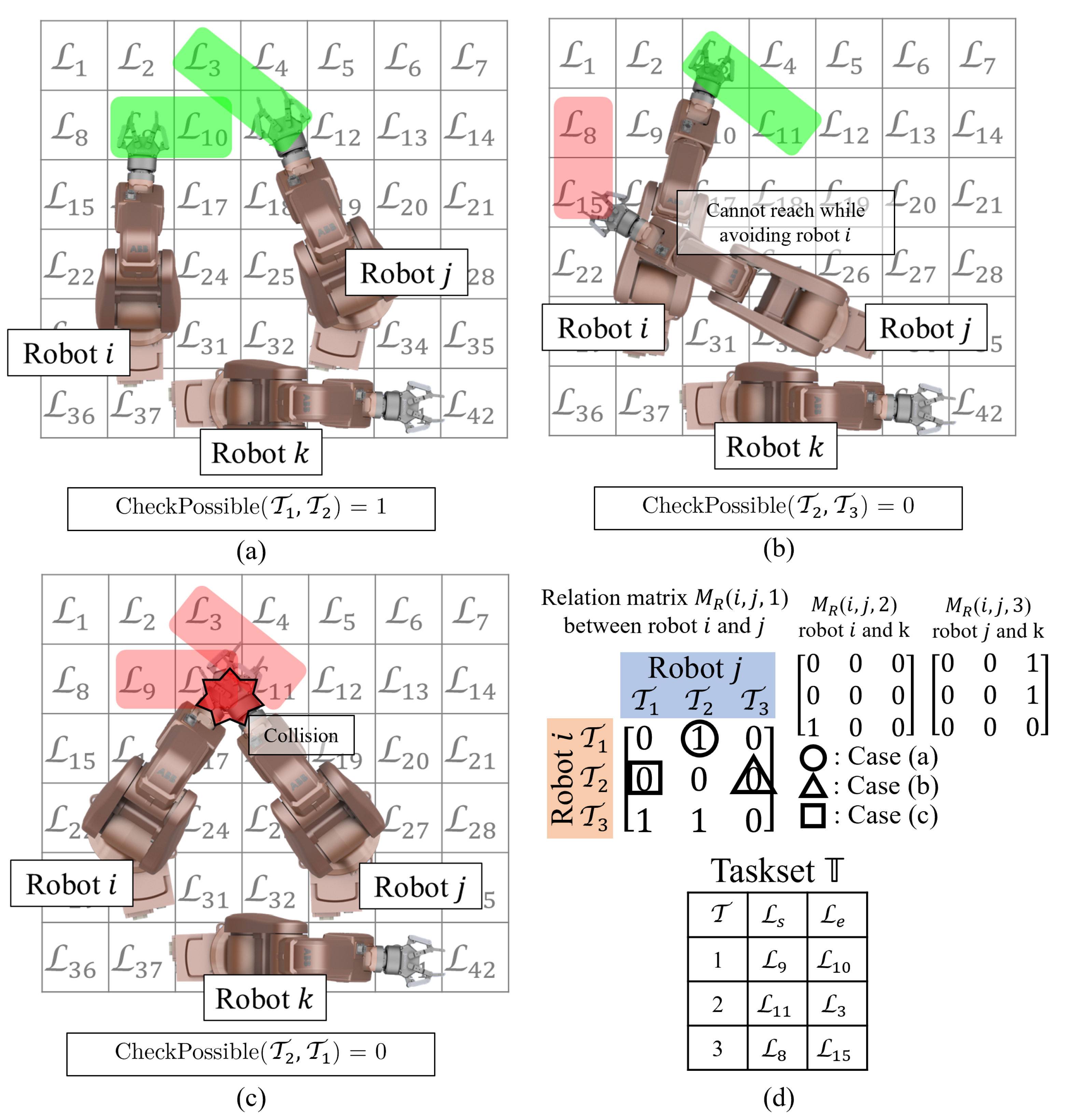
2.3.2. Kinematic Constraint

Due to the use of a robot in a controlled environment, kinematic constraints are generated. The constraints are affected by the configuration of the robot, predefined tasks, and the locations where the tasks are performed. Those components are not changed unless the configuration of robot or environment is not changed. Therefore, once the constraints are calculated before solving the problem, it does not need to be calculated while solving the optimization problem.
To minimize makespan, it is important that both robotic arms are performing tasks concurrently as much as possible. Using kinematic information, it is possible to calculate whether robotic arms can perform two specific tasks simultaneously, and it can be represented as a hashtable-like matrix called a Relation Matrix.
Definition 2.
A Relation Matrix M R is a binary matrix where the rows represent one arm’s capability to execute tasks and the columns represent the other arm’s capability to execute tasks. If there exists a nonzero element in M R ( i , j ) , then one arm can perform T i while the other arm can also conduct T j . If there are n tasks in T , the size of M R is n × n in the case where two robotic arms are used. When the number of robots is m, M R has a dimension of n × n × m C 2 .
An example of the case with three machines (robotic arm) describing the Relation Matrix is shown in Figure 1. A simple t a s k s e t T is defined in Figure 1d, and examples of obtaining the components of M R are presented in (a)–(c). In this example, M R has ( 3 × 3 × 3 C 2 ) dimension, because the number of tasks are 3, and robots are 3. To check whether the robot i and robot j can perform specific tasks simultaneously, we define CheckPossible ( T i , T j ) , and it returns the value 1 when possible and 0 when not. T i , T j is the task conducted by robot i and j, respectively. The function CheckPossible ( T i , T j ) checks two components: reachability and collision between two robots. Reachability can be calculated by discretizing the Cartesian space into smaller cubes and by verifying if all points on a surface of a sphere inside the cube can be reached [46]. However, in our environment, cooking materials, appliances, and tools are placed at specific locations, so it does not need to consider the entire Cartesian space. Figure 1b shows the case where the right arm cannot perform T 3 because it cannot reach the location. In this case, the value of CheckPossible ( T 2 , T 3 ) becomes 0 and so does M R ( 2 , 3 , 1 ) .
The second thing checked by CheckPossible ( T i , T j ) is the collision between two arms, which is affected by kinematic constraints such as the configuration of the robot. Finding out the collisions between manipulator is one of the research fields in robotics, but it is not the main scope of our work. In more detail, the state-of-the-art method [47] can be applied. Figure 1c shows the case in which the two arms collide with each other. In this case, the value of M R ( 2 , 1 , 1 ) become 0 because CheckPossible ( T 2 , T 1 ) is 0. Figure 1a shows that this case is possible, so the value M R ( 1 , 2 , 1 ) is 1. M R ( i , k , 2 ) , M R ( j , k , 3 ) also can be obtained using the method above. Following the method described above, M R can be found before the start of the optimization process. In the next section, the method describing how to apply the information from M R to the optimization problem will be presented.

3. Task Scheduling with Mixed-Integer Programming

In this section, the two-step task-scheduling algorithm presented in Section 2.1 considering the unique constraints mentioned in Section 2.3 is presented. The overall algorithm is shown in Algorithm 1. Once a t a s k s e t T , such as the one shown in Table 1, is prepared, the proposed mixed-integer optimization is conducted to determine the cooking sequences of all of the tasks. Thanks to the disjunctive constraints introduced to express the constraints, the optimization process can be formulated in a systematic way. After an optimal task is selected, the arms are assigned for each task based on the moving distance optimization criterion. Moreover, we present the subproblem optimization strategy in this section, which makes it possible to realize the optimization framework that can produce a feasible solution in run-time.

3.1. Task Scheduling with the Kinematic Constraints

While arranging multiple tasks, there are task pairs that cannot be performed simultaneously due to kinematic constraints. In this case, only part of the constraints in the task pairs set must hold, and it is called disjunctive constraints [48]. To schedule tasks in T , suppose that there are n dishes( D ). Each T j i (jth task in ith dish) must be performed on each D i . Suppose that the ith dish has x i tasks; then, the range of j is expressed as m 1 i , m x i i . For example, m 1 2 = 16 ,   m 7 2 = 22 ,   m 10 3 = 32 in Table 1. Suppose t j i is the start time of jth task ( T j i ) on the ith dish ( D i ). τ j i means the time duration of T j i in D i . Because T j + 1 i cannot start until T j i is finished, we can obtain the constraints below. c j i is also considered in the constraint, as explained in Section 2.3.1.
t j + 1 i t j i + τ j i when c j i = 0 , for j = m 1 i , , m x i i t j + 1 i = t j i + τ j i when c j i = 1 , for j = m 1 i , , m x i i
Equation (1) reflects the dependency constraint, but the kinematic constraints still need to be reflected. Assuming that M R is precalculated, it can be known which tasks cannot be performed simultaneously. For setting the constraints, the cases to be found are the cases that cannot be performed simultaneously. We describe this situation as the ‘tasks are in collision’. Therefore, an equation is formulated to avoid the collision of the task. Suppose that T i and T j are checked for collisions. For example, when M R ( i , j ) = 0 and M R ( j , i ) = 1 , T i and T j will not collide with each other because T j can be performed by the right arm and T i can be carried out by the left arm. Therefore, to find collision tasks, the cases M R ( i , j ) = 0 and M R ( j , i ) = 0 should be found. This task collision checking process is shown in Algorithm 2 lines 7 to 10 and in Algorithm 2 lines 5 to 8. For all tasks and dishes in the T , the collision checking process needs to be performed to find all collision task pairs. Suppose that T k a in D a and T l b in D b ( a , b , k , l N : a , b [ 1 , n ] , k [ 1 , m a ] , l [ 1 , m b ] ) determine that both cannot be performed simultaneously; then, ( a , b , k , l ) is inserted into the list of conflicting tasks is C .
After finding all colliding task pairs, the collision avoidance constraints need to be set. To set collision avoidance constraints, disjunctive constraints δ k l a b is introduced [49]. δ k l a b is a binary variable, and its value becomes 1 when T k a is processed before T l b starts ( t k a t l b ) and 0 when t k a t l b . Using δ k l a b , the constraints can be written as below. B is a sufficiently large positive number.
t l b t k + 1 a + B ( 1 δ k l a b ) 0 , t k a t l + 1 b + B δ k l a b 0 , for ( a , b , k , l ) N : ( a , b ) [ 1 , n ] , k [ 1 , m a ] , l [ 1 , m b ] .
Our goal is to minimize the time the last task to finish. t C is defined as makespan, and it is greater than or equal to the completion time of each dish. It can be expressed t C t x i i + τ x i i for all D when each D i has x i tasks. The list of conflicting tasks C was defined above, and the collision avoidance constraints need to be added with all of the components in C . If the number of components of C is k, then the constraint 2 k is added. If the number of D is n, then the total number of constraints are n + 2 · i = 1 n x i + 2 k . The formulation that considers every constraints is as follows:
minimize t t C subject to t C t x i i + τ x i i for i = 1 , , n t j i 0 t j + 1 i t j i + τ j i when c j i = 0 , for i = 1 , , n , j = m 1 i , , m x i i t j + 1 i = t j i + τ j i when c j i = 1 , for i = 1 , , n , j = m 1 i , , m x i i t l b t k + 1 a + B ( 1 δ k l a b ) 0 t k a t l + 1 b + B δ k l a b 0 f o r ( a , b , k , l ) C δ k l a b { 0 , 1 } .
Algorithm 2: Optimization solver.
1:
procedure SolveOptimization ( T )
2:
     T = { D } = { ( T , τ , L s , L e , A ) }
3:
     n number of D
4:
     x i number of T j i in D i
5:
    for a = 1 to n and b = 1 to n do
6:
        for k = m 1 a to m x a a and l = m 1 b to m x b b  do
7:
           if  M R ( k , l ) = 0   and   M R ( l , k ) = 0  then
8:
                C .insert ( a , b , k , l )
9:
    find minimize t     t C
10:
          subject to t C t x i i + τ x i i f o r i = 1 , , n
11:
                           t j i 0
12:
                           t j + 1 i t j i + τ j i when   c j i   =   1 ,   for   i   =   1 ,   ,   n ,   j   =   m 1 i ,   ,   m x i i
13:
                           t j + 1 i = t j i + τ j i when c j i   =   0 ,   for   i   =   1 ,   ,   n ,   j   =   m 1 i ,   ,   m x i i
14:
                           t l b t k + 1 a + B ( 1 δ k l a b ) 0
15:
                           t k a t l + 1 b + B δ k l a b 0   for   ( a , b , k , l ) C
16:
                           δ k l a b { 0 , 1 } .
17:
    for j = 1 to N do
18:
         D .insert ( p ( L s , j ) p ( L e , j + 1 ) )
19:
    find minimize L ( T ) , R ( T )     D t
20:
          subject to     D t L ( T ) · D
21:
                            D t R ( T ) · D
22:
                            L ( T j ) + R ( T j ) = A j   for  j   =  1 , , N
23:
                            L ( T l ) = 1 ,  R ( T l ) = 0 ,  L ( T k ) = 0 ,  R ( T k ) = 1 f o r ( k ,  l ) C
24:
                                when  M R   ( k , l ) = 0  and   L ( T j ) + R ( T j ) = 1 .
25:
    return  t , L ( T ) , R ( T )

3.2. Assigning Arm to the Tasks

In this section, the formulation that assigns the robot arms to each task and minimizes the transition distance between tasks is proposed. The t j i values for all T j i are decided in Section 3.1. Thus, the results from Section 3.1 is used as the input of our second-step formulation. The constraint of the second-step formulation is mainly related to A j i , which is the number of arms needed to proceed T j i . Let the sum of the number of tasks be N = i = 1 n x i . Then, we can define two binary vectors to assign tasks to the left and right arms, L ( T )   and   R ( T ) , and their size is N. If L ( T j i ) = 1 , the left arm is performing T j i , and 0 means that T j i is not processed by the left arm. This definition gives the condition L ( T j i ) + R ( T j i ) = A j i for j = 1 , , N . When A j i = 2 or 0, L ( T j i ) and R ( T j i ) are determined to be (1,1) and (0,0), respectively. However, in the case where A j i = 1 , additional constraints are needed. From the result in Section 3.1, the task pairs in that process can be concurrently seen. Assuming that T k a and T l b need to be processed at the same time and A k a = 1 and A l b = 1 , it must be checked whether M R ( T k a , T l b ) = 1 or M R ( T l a , T k b ) = 1 . If the former case, the result becomes L ( T l b ) = 1 , R ( T l b ) = 0 , L ( T k a ) = 0 , R ( T k a ) = 1 , and if the latter, it becomes 0, 1, 1, and 0, respectively. From A , most of constraints are decided. However, in the case of T j i having no pairs of tasks performed concurrently and A j i = 1 , additional constraints are needed.
For additional constraints, when T j + 1 is the next sequence of T j , the distance between L e , j and L s , j + 1 is considered. Let us define p ( L s , j ) , p ( L e , j ) as the Cartesian coordinates of L s , j and L e , j . Additionally, we define D as the set of distances between the locations. If we define d = p ( L s , j + 1 ) p ( L e , j ) , then we can add d to D . Because the sizes of L ( T ) and R ( T ) are N, the number of d can be obtained N 1 . To make the dimensions of D the same as L ( T ) and R ( T ) , we add an initial location. Then, the distance between the initial position and first task can be added into D , making the size of D N. The moving distance does not need to be considered when the robot arm will not perform T j i ; when A j i = 0 , it has to be zero. Reflecting this condition, the moving distance of the left arm is L ( T ) · D and that of the right arm is R ( T ) · D . One condition for these equations to be established is that the left or right arms should not be moved when L ( T j i ) = 0 , R ( T j i ) = 0 , respectively. From the result of the cross product, the constraints D t L ( T ) · D , D t R ( T ) · D when D t is to be minimized. The formulation that considers every constraint is as follows:
minimize L ( T ) , R ( T ) D t subject to D t L ( T ) · D D t R ( T ) · D L ( T j ) + R ( T j ) = A j for j = 1 , , N L ( T l ) = 1 , R ( T l ) = 0 , L ( T k ) = 0 , R ( T k ) = 1 for ( k , l ) C when   M R ( k , l ) = 1   and   L ( T j ) + R ( T j ) = 1 .
The whole optimization process is shown in Algrothm 2. Line 5 ∼ 8 shows the collision check process of the task in Section 3.1 before optimization. Through this process, the list of conflicting tasks C can be obtained. After that, the sequence of time t can be obtained through the solving stage 1 in Section 3.1 and is shown in lines 9 ∼ 16. Using the collision information, the distance vector D is calculated in lines 17 ∼ 18. Stage 2 in Section 3.2 is processed in lines 19 ∼ 25.

3.3. Subproblem Optimization Strategy

This section deals with how to apply the subproblem optimization strategy by dividing one T into several. In the previous section, if the whole T is applied to the formulation, the actual work cannot begin until all processes have been computed. In the real process, it is necessary to modify or add a task in the middle, so online planning is necessary. We established a strategy to divide T to carry out online planning, which was one of the limitations of the previous study [25].
The process of executing the subproblem optimization strategy is in Algorithm 3. Our first goal is to recursively divide T into subproblems. S is set as the maximum number of tasks in a subproblem in line 2. In line 4, G is set as a group of subproblems. Let the ith component in G be defined as T i . Divide ( T i ) divides T i into several proper size of subproblem. The method to divide T i is as follows. If T i contains m tasks and n dishes and T i is divided into s segments, then one segment of T contains m / s tasks when m / s N . In each segment, the tasks located in the first sequence of each dish are gradually filled. In the case of m / s N , each segment contains a different number of tasks. Moreover, considering the continuity of tasks, the tasks that cannot be separated from each other should be placed in one segment. If T i is divided into s problems, the outputs become T i , 1 , , T i , s , and these are described in line 8. The each components of outputs T i , 1 , , T i , s are used as input of Divide in the next step. This step (lines 5 to 10) is executed until the number of tasks in all components of G is reduced under S .
After dividing the problem, the optimization of all subproblems should be solved. Let the ith t, L ( T ) , and  R ( T ) be defined as t s e g , i , L ( T ) s e g , i , and  R ( T ) s e g , i , respectively. Then, the result of optimizations of T i is that t s e g , i , L ( T ) s e g , i , R ( T ) s e g , i can be obtained from SolveOptimization( T i ). The final results t , L ( T ) , R ( T ) are the stack of each segmented result.
Algorithm 3: Subproblem optimization strategy.
1:
T = { ( T , τ , L s , L e , A ) }
2:
S Maximum number of tasks in segmented   T
3:
G Group of segmented   T
4:
G .insert( T )
5:
while NumberOfTasks ( T i G ) > S do
6:
     g Empty list
7:
    for  T i in   G  do
8:
         T i , 1 , , T i , s Devied ( T i )
9:
        g.insert( T i , 1 , , T i , s )
10:
     G g
11:
for T i   in   G   do
12:
     t s e g , i , L ( T ) s e g , i , R ( T ) s e g , i SolveOptimization( T i )
15:
    t.insert ( t s e g , i )
16:
     L ( T ) .insert ( L ( T ) s e g , i )
17:
     R ( T ) .insert ( R ( T ) s e g , i )
18:
end for

4. Experiment

In this section, the results of the test Algorithms 1 and 3 are presented. In the simulated experiments, the results were observed when changing the number of tasks and the number of segments. The optimization solver used is MOSEK [50], running on a desktop computer with a CPU of Intel Core i7 10700K @ 3.80GHz and 32GB of RAM at 2666 MHz.

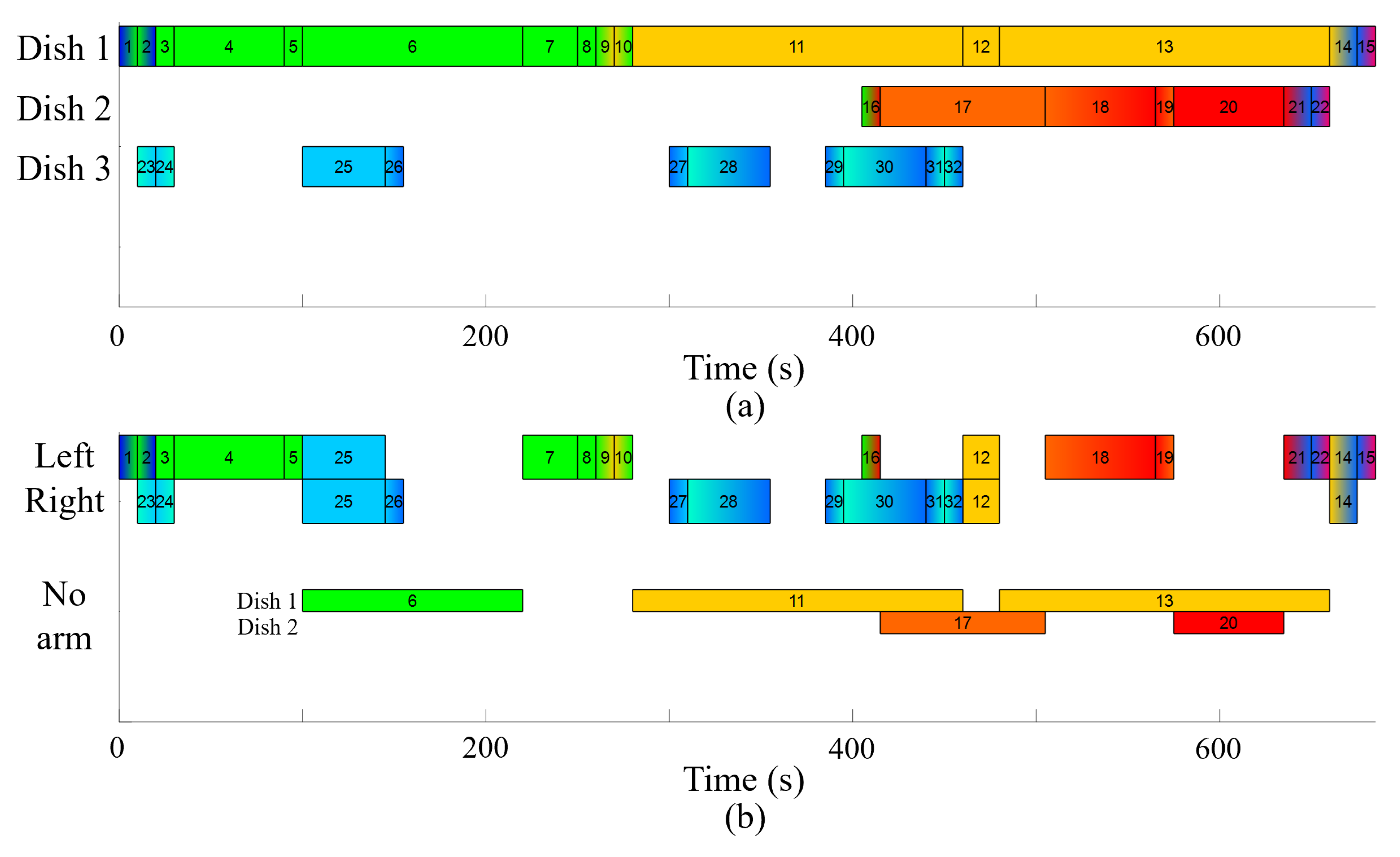
4.1. Task Scheduling and Assigning Arm

Using the the taskset T data in Table 1 as the input, Algorithm 1 was tested in a realistic environment. The cooking robot in the environment is made up of 11 degrees of freedom (DOF) dual arms, where there are five DOFs per arm with another revolute joint that couples the two arms at the center of the body. This robot was designed and analyzed in our previous work [51]. Additionally, the tables with tools for cooking surround the robot. Figure 2 shows the environment used for the experiments. The workspace is segmented into several spaces, and specific tasks are performed at that location. The yellow boxes in Figure 2 represent each location, and the indices were set for convenience, which are the numbers in the white box in (b). We assume that one task can have performed in 1 ∼ 2 locations, start and end locations (e.g., moving the bowl from the 6th location to the 7th location). Depending on the robot configuration, the table is arranged in a way that the robot can access all locations. Thanks to the coupling joint in the waist of the robot, a single arm can access all locations easily.
The results of the experiment are shown in Figure 3. Figure 3a shows the result of the first step of the optimization process in Section 3.1, (b) shows the result of the second step in Section 3.2. Each rectangle represents all T in T and the same color represents the same location of the task. If L s L e in one T , then the colors change gradually in one box. In Figure 3a, the result did not violate any kinematic constraints and dependencies of T . In Figure 3b, all T are assigned to the left and right arms properly. The task needs two arms (e.g., T 12 , T 14 , and T 25 ) and no arm (e.g., T 6 , T 11 , T 13 , T 17 , and T 20 ) are also well assigned following the sequences. Moreover, the continuity is well reflected in the result. The tasks where c = 1 were T 5 , T 6 , T 9 to T 12 , T 17 , and T 20 . The result shows that T 5 to T 7 , T 9 to T 13 , T 17 , T 18 , T 20 , and T 21 are consecutive, so it can be seen that continuity is well reflected.

4.2. Comparison with Conventional Algorithm

The experiments were performed to compare the performance of our algorithm with the conventional algorithm. Let us define an n × m problem when n jobs are conducted on m machines. The experiments consist of problems of twelve sizes, which are 2 × 2 , 3 × 2 , 4 × 2 , 5 × 2 , 2 × 3 , 3 × 3 , 4 × 3 , 5 × 3 , 2 × 4 , 3 × 4 , 4 × 4 , and 5 × 4 , and each set consists of ten problem instances. As mentioned in Section 2.2, the conventional algorithm used a pre-assigned machine for a specific operation. Therefore, while testing the conventional algorithm, a robotic arm is assigned to cook specific dishes. Additionally, our algorithm did not assign a robotic arm to a specific task. In case of number of machine is more than two, the process adding constraint (lines 20 to 24 in Algorithm 2) is executed m C 2 times when m machines exist. For example, for n × 3 problem, the constraints from the pairs of (1st, 2nd), (1st, 3rd), (2nd, 3rd) robots will be added in the formula. Table 2 shows the result of the comparison between conventional algorithm and ours. Opt means the number of instances proved to optimality. The results show that our algorithm can obtain a better or same makespan than the conventional algorithm. The reason for this result is that if the number of machines (robotic arms) is insufficient compared with the number of jobs (dishes), it is more advantageous in makespan to allocate robot arms later. In case of run-time, when the size of the problem is small, there are cases where it is larger because of the second step of our algorithm (lines 19 to 25 in Algorithm 2). However, as the problem size increases, the run-time of our algorithm also had advantages because pre-defined machines create more constraints using the conventional method.

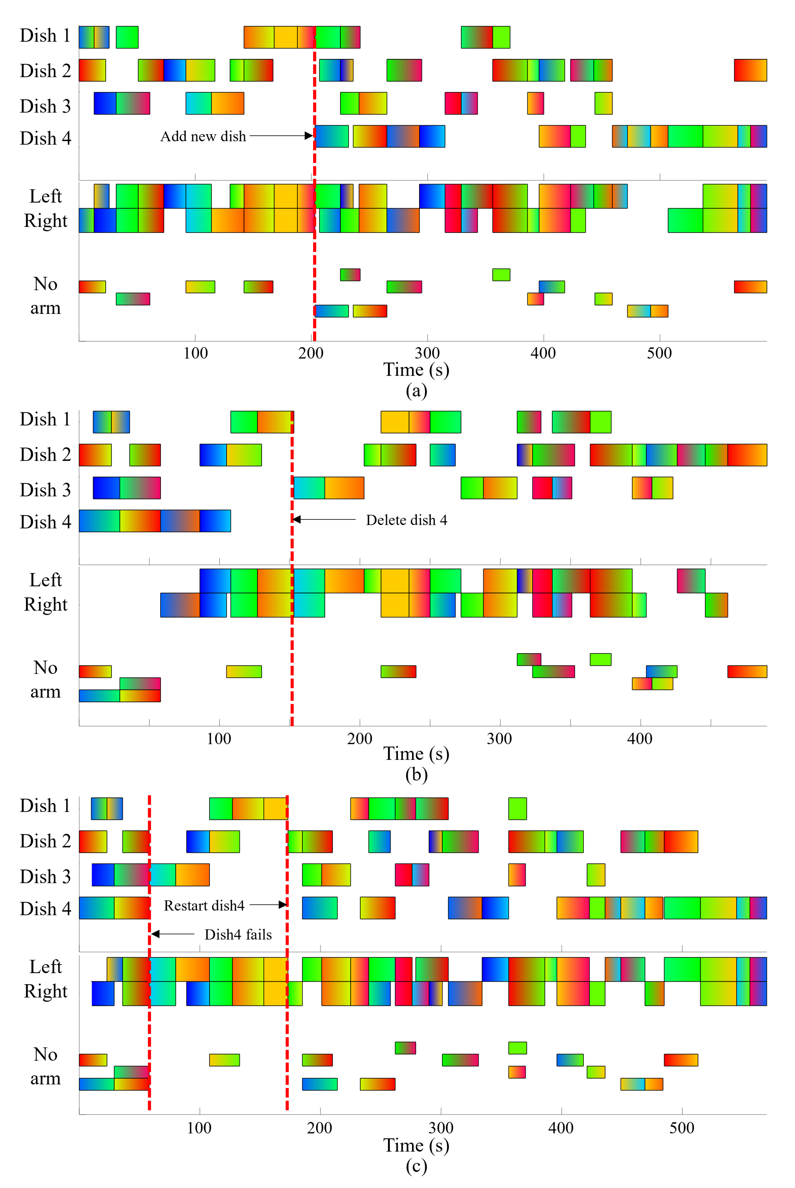
4.3. Subproblem Optimization Strategy

In this section, Algorithm 3 is validated. It is obvious that the result of the makespan in the segmented case is longer than in the non-segmented case because the task that can be performed at the same time may not be performed simultaneously. However, the advantage in the run-time of the algorithm can be expected. In general, when computing optimization, the computation time increases exponentially with each process step [52]. As the number of tasks increases, the probability of the number of collision cases between tasks also increases. According to Equation (2), if the length of C increases, then the number of constraints increase twice. By dividing the T , the number of constraints in MIP will be decreased. The experiments for verifying these are conducted as followed.
To see the correlation between the number of tasks and the optimization result, experiments were conducted using 30 to 120 tasks. Each T contained 2 dishes and was divided until each segments included 10 tasks ( S = 10 ). Figure 4 shows the experimental results, and the experiments were conducted 50 times to compare the average. When looking at the cases in which the number of tasks in T is less than 70 in Figure 4a, the total elapsed time ( t C + run time) increased by 3.36% on average when T was divided compared with the case in which T was not divided. However, as the size of T increases, the computational time of the full case exponentially increases, as shown in Figure 4b. It causes opposite trends, as shown in Figure 4a, when the number of tasks exceeds 70. The total time elapsed decreased by 12.4% on average when T was divided. It can be seen through the result that the subproblem strategy reduces not only the computation time but also the overall time in the large problem. When comparing Figure 4b,c, the segmented result is much smaller relative to the full-sized result.
Figure 4b shows the result of using full-sized T . The computational times taken to solve collision checking and MIP (including the first and second steps) are displayed together. However, in the case of (b), the run-time of the collision check is much more than that of MIP. It can be seen that, when the problem size becomes big, the collision checking process becomes the most computationally expensive. Thus, when the run-time of a big problem is considered, considering only the computational time of the collision checking process can be acceptable. Figure 4c shows the result of using segmented T . In this figure, it can be seen that the run-time of the collision checking process is significantly reduced. In the case of T that has 120 tasks, run-time is reduced from 499 s to 2.433 s. The average reduced run-time is 73.81% and 98.9% when the number of tasks is more than 60. Through the experimental results, it can be seen that the optimization strategy for subproblems has an advantage in terms of computational time and total elapsed time, especially when the size of the problem is large. It can be expected that this strategy will be optimized to perform tremendous cooking tasks that humans cannot perform.
To examine how the subproblem optimization strategy can respond to change of task in the middle of executing, three cases with changing situations are verified. T used in this experiment is randomly generated, and it contains four dishes. D 1 contains 10 tasks, D 2 has 15, D 3 has 10, and D 4 has 13. The first case is to add one more plate in the middle of the process. If it is assumed that the robot is working in a restaurant kitchen, this can be happened when a customer orders an additional dish. In Figure 5a, the result of the first case is shown. In the first part of the timeline, only D 1 to D 3 are processed. At the time indicated by the red dashed line, the command was given to start cooking D 4 . As shown in the figure, D 4 started successfully and finished the entire process. The second case is when the dish is removed in the middle of the process. This situation can happen when the order is canceled. In Figure 5b, D 1 to D 4 are processed simultaneously by the robot. However, D 4 is removed after the time indicated by the red dashed line. After that, D 4 is not processed at all. The last case is that one dish is restarted after a failure. It is assumed that the situation is such that if the robot drops any ingredients earlier during cooking, then cooking has to be restarted from the beginning. There are two red dashed line in Figure 5c. The line on the left indicates the time at which the robot fails D 4 . After recognizing the failure, the restart command is given in the second red line. From this, D 4 is restarted again from the beginning. Through all three cases, it is shown that our algorithm can conduct online planning.

5. Conclusions

In this article, a framework is proposed that can optimally schedule multiple cooking tasks simultaneously. Two mixed-integer programs are formulated to schedule a sequence of tasks and to assign robot arms to tasks. For executing online planning, a subproblem optimization strategy is also proposed. Even though the makespan increased by 6.02%, the run-time was significantly reduced by 98.9%, so the total elapsed time was reduced by 7.89% in a big problem with over 110 tasks.
The approach was validated on a real-sized t a s k s e t and segmented t a s k s e t . Moreover online planning was validated in situations where tasks are suddenly reordered. Although this work was proposed for the scheduling of cooking tasks, it can be applied to any situation that needs to be optimized, such as the scheduling of work in a warehouse using multiple mobile robots, where more than one robot is used and the workspace is shared. Future work includes cooking in a real environment with a vision-recognition system that can detect tasks that fail.

Author Contributions

Conceptualization, J.-s.Y., T.A.L. and M.S.A.; methodology, J.-s.Y. and T.A.L.; software, J.-s.Y. and T.A.L.; validation, J.-s.Y. and T.A.L.; formal analysis, J.-s.Y. and T.A.L.; investigation, J.-s.Y. and T.A.L.; resources, J.-s.Y.; data curation, J.-s.Y.; writing—original draft preparation, J.-s.Y. and T.A.L.; writing—review and editing, H.C., M.S.A., D.N., H.N.T., E.A., N.P. and F.Y.; visualization, J.-s.Y., M.D.; supervision, D.H. and H.M.; project administration, J.-s.Y. and H.M.; All authors have read and agreed to the published version of the manuscript.

Funding

This research was supported by the MOTIE (Ministry of Trade, Industry, and Energy) in Korea, under the Fostering Global Talents for Innovative Growth Program (P0008746) supervised by the Korea Institute for Advancement of Technology (KIAT).

Institutional Review Board Statement

Not applicable.

Informed Consent Statement

Not applicable.

Conflicts of Interest

The authors declare no conflict of interest.

References

  1. Caldwell, D.G. Robotics and Automation in the Food Industry: Current and Future Technologies; Elsevier: Amsterdam, The Netherlands, 2012. [Google Scholar]
  2. Kuo, C.F.; Nelson, D.C. A simulation study of production task scheduling for a university cafeteria. Cornell Hosp. Q. 2009, 50, 540–552. [Google Scholar] [CrossRef]
  3. Watanabe, Y.; Nagahama, K.; Yamazaki, K.; Okada, K.; Inaba, M. Cooking behavior with handling general cooking tools based on a system integration for a life-sized humanoid robot. Paladyn, J. Behav. Robot. 2013, 4, 63–72. [Google Scholar] [CrossRef]
  4. Bollini, M.; Tellex, S.; Thompson, T.; Roy, N.; Rus, D. Interpreting and Executing Recipes with a Cooking Robot; Experimental Robotics; Springer: Berlin/Heidelberg, Germany, 2013; pp. 481–495. [Google Scholar]
  5. Wang, H.; Zhao, W.; Li, B.; Lin, X.; Zhang, D. Dynamic analysis and robust reliability design of pan mechanism for a cooking robot. In Proceedings of the 2009 IEEE International Conference on Robotics and Biomimetics (ROBIO), Guilin, Guangxi, 13–19 December 2009; pp. 1996–2001. [Google Scholar]
  6. Beetz, M.; Klank, U.; Kresse, I.; Maldonado, A.; Mösenlechner, L.; Pangercic, D.; Rühr, T.; Tenorth, M. Robotic roommates making pancakes. In Proceedings of the 2011 11th IEEE-RAS International Conference on Humanoid Robots, Bled, Slovenia, 26–28 October 2011; pp. 529–536. [Google Scholar]
  7. Inagawa, M.; Takei, T.; Imanishi, E. Japanese Recipe Interpretation for Motion Process Generation of Cooking Robot. In Proceedings of the 2020 IEEE/SICE International Symposium on System Integration (SII), Honolulu, HI, USA, 12–15 January 2020; pp. 1394–1399. [Google Scholar]
  8. (ENG) ‘CLOi’s Table Zone’, Futuristic Restaurant at CES. 2020. YouTube. 2022. Available online: https://www.youtube.com/watch?v=vsZ_HUAPXL8 (accessed on 14 March 2022).
  9. Samsung Bot Chef at CES 2020. YouTube. 2022. Available online: https://www.youtube.com/watch?v=OwA6-b1Z7aQ (accessed on 14 March 2022).
  10. Aeronautiques, C.; Howe, A.; Knoblock, C.; McDermott, I.D.; Ram, A.; Veloso, M.; Weld, D.; SRI, D.W.; Barrett, A.; Christianson, D.; et al. PDDL|The Planning Domain Definition Language. Tech. Rep. 1998. [Google Scholar]
  11. Jeon, J.; Jung, H.r.; Yumbla, F.; Luong, T.A.; Moon, H. Primitive Action Based Combined Task and Motion Planning for the Service Robot. Front. Robot. AI 2022, 9, 713470. [Google Scholar] [CrossRef] [PubMed]
  12. Jiang, Y.q.; Zhang, S.q.; Khandelwal, P.; Stone, P. Task planning in robotics: An empirical comparison of PDDL-and ASP-based systems. Front. Inf. Technol. Electron. Eng. 2019, 20, 363–373. [Google Scholar] [CrossRef]
  13. Manso, L.J.; Bustos, P.; Alami, R.; Milliez, G.; Núnez, P. Planning human–robot interaction tasks using graph models. In Proceedings of the International Workshop on Recognition and Action for Scene Understanding (REACTS 2015), Malta, Malta, 5 September 2015; pp. 15–27. [Google Scholar]
  14. Ayunts, E.; Panov, A.I. Task planning in “Block World” with deep reinforcement learning. In First International Early Research Career Enhancement School on Biologically Inspired Cognitive Architectures; Springer: Berlin/Heidelberg, Germany, 2017; pp. 3–9. [Google Scholar]
  15. Lee, H. Learning Representations and Models of the World for Solving Complex Tasks; NVIDIA: Santa Clara, CA, USA, 2021. [Google Scholar]
  16. Bengio, Y.; Lodi, A.; Prouvost, A. Machine learning for combinatorial optimization: A methodological tour d’horizon. Eur. J. Oper. Res. 2021, 290, 405–421. [Google Scholar] [CrossRef]
  17. Kleinert, T.; Labbé, M.; Ljubić, I.; Schmidt, M. A survey on mixed-integer programming techniques in bilevel optimization. EURO J. Comput. Optim. 2021, 9, 100007. [Google Scholar] [CrossRef]
  18. Leal, M.; Ponce, D.; Puerto, J. Portfolio problems with two levels decision-makers: Optimal portfolio selection with pricing decisions on transaction costs. Eur. J. Oper. Res. 2020, 284, 712–727. [Google Scholar] [CrossRef]
  19. Bastos, L.S.; Marchesi, J.F.; Hamacher, S.; Fleck, J.L. A mixed integer programming approach to the patient admission scheduling problem. Eur. J. Oper. Res. 2019, 273, 831–840. [Google Scholar] [CrossRef]
  20. Yanıkoğlu, I.; Kuhn, D. Decision rule bounds for two-stage stochastic bilevel programs. SIAM J. Optim. 2018, 28, 198–222. [Google Scholar] [CrossRef]
  21. Lima, R.M.; Grossmann, I.E. Computational Advances in Solving Mixed Integer Linear Programming Problems; AIDAC: Rome, Italy, 2011. [Google Scholar]
  22. Leung, J.M.; Zhang, G.; Yang, X.; Mak, R.; Lam, K. Optimal cyclic multi-hoist scheduling: A mixed integer programming approach. Oper. Res. 2004, 52, 965–976. [Google Scholar] [CrossRef]
  23. Sawik, T. Batch versus cyclic scheduling of flexible flow shops by mixed-integer programming. Int. J. Prod. Res. 2012, 50, 5017–5034. [Google Scholar] [CrossRef]
  24. Che, A.; Lei, W.; Feng, J.; Chu, C. An improved mixed integer programming approach for multi-hoist cyclic scheduling problem. IEEE Trans. Autom. Sci. Eng. 2013, 11, 302–309. [Google Scholar] [CrossRef]
  25. Yi, J.S.; Ahn, M.S.; Chae, H.; Nam, H.; Noh, D.; Hong, D.; Moon, H. Task Planning with Mixed-Integer Programming for Multiple Cooking Task Using dual-arm Robot. In Proceedings of the 2020 17th International Conference on Ubiquitous Robots (UR), Kyoto, Japan, 22–26 June 2020; pp. 29–35. [Google Scholar]
  26. Huang, K.L.; Liao, C.J. Ant colony optimization combined with taboo search for the job shop scheduling problem. Comput. Oper. Res. 2008, 35, 1030–1046. [Google Scholar] [CrossRef]
  27. Zhang, R.; Song, S.; Wu, C. A hybrid artificial bee colony algorithm for the job shop scheduling problem. Int. J. Prod. Econ. 2013, 141, 167–178. [Google Scholar] [CrossRef]
  28. Wang, L.; Zhou, G.; Xu, Y.; Wang, S.; Liu, M. An effective artificial bee colony algorithm for the flexible job-shop scheduling problem. Int. J. Adv. Manuf. Technol. 2012, 60, 303–315. [Google Scholar] [CrossRef]
  29. Nakano, R.; Yamada, T. Conventional genetic algorithm for job shop problems. ICGA 1991, 91, 474–479. [Google Scholar]
  30. Della Croce, F.; Tadei, R.; Volta, G. A genetic algorithm for the job shop problem. Comput. Oper. Res. 1995, 22, 15–24. [Google Scholar] [CrossRef]
  31. Sha, D.; Hsu, C.Y. A hybrid particle swarm optimization for job shop scheduling problem. Comput. Ind. Eng. 2006, 51, 791–808. [Google Scholar] [CrossRef]
  32. Lin, T.L.; Horng, S.J.; Kao, T.W.; Chen, Y.H.; Run, R.S.; Chen, R.J.; Lai, J.L.; Kuo, I.H. An efficient job-shop scheduling algorithm based on particle swarm optimization. Expert Syst. Appl. 2010, 37, 2629–2636. [Google Scholar] [CrossRef]
  33. Yazdani, M.; Amiri, M.; Zandieh, M. Flexible job-shop scheduling with parallel variable neighborhood search algorithm. Expert Syst. Appl. 2010, 37, 678–687. [Google Scholar] [CrossRef]
  34. Adibi, M.; Zandieh, M.; Amiri, M. Multi-objective scheduling of dynamic job shop using variable neighborhood search. Expert Syst. Appl. 2010, 37, 282–287. [Google Scholar] [CrossRef]
  35. Adams, J.; Balas, E.; Zawack, D. The shifting bottleneck procedure for job shop scheduling. Manag. Sci. 1988, 34, 391–401. [Google Scholar] [CrossRef]
  36. Beck, J.C. Solution-guided multi-point constructive search for job shop scheduling. J. Artif. Intell. Res. 2007, 29, 49–77. [Google Scholar] [CrossRef]
  37. Beck, J.C.; Feng, T.; Watson, J.P. Combining constraint programming and local search for job-shop scheduling. INFORMS J. Comput. 2011, 23, 1–14. [Google Scholar] [CrossRef] [Green Version]
  38. Gromicho, J.A.; Van Hoorn, J.J.; Saldanha-da Gama, F.; Timmer, G.T. Solving the job-shop scheduling problem optimally by dynamic programming. Comput. Oper. Res. 2012, 39, 2968–2977. [Google Scholar] [CrossRef]
  39. Meng, L.; Zhang, C.; Ren, Y.; Zhang, B.; Lv, C. Mixed-integer linear programming and constraint programming formulations for solving distributed flexible job shop scheduling problem. Comput. Ind. Eng. 2020, 142, 106347. [Google Scholar] [CrossRef]
  40. Ku, W.Y.; Beck, J.C. Mixed integer programming models for job shop scheduling: A computational analysis. Comput. Oper. Res. 2016, 73, 165–173. [Google Scholar] [CrossRef] [Green Version]
  41. Pan, J.C.H.; Chen, J.S. Mixed binary integer programming formulations for the reentrant job shop scheduling problem. Comput. Oper. Res. 2005, 32, 1197–1212. [Google Scholar] [CrossRef]
  42. Van Hulle, M.M. A goal programming network for mixed integer linear programming: A case study for the job-shop scheduling problem. Int. J. Neural Syst. 1991, 2, 201–209. [Google Scholar] [CrossRef]
  43. Liao, C.J.; You, C.T. An improved formulation for the job-shop scheduling problem. J. Oper. Res. Soc. 1992, 43, 1047–1054. [Google Scholar] [CrossRef]
  44. our over Coffee Drip Brewing Guide—How to Make Pour over Coffee. Blue Bottle Coffee. 2022. Available online: https://bluebottlecoffee.com/brew-guides/pour-over (accessed on 14 March 2022).
  45. Chinese Chicken Salad. The Cheesecake Factory. 2022. Available online: https://www.thecheesecakefactory.com/recipes/chinese-chicken-salad (accessed on 14 March 2022).
  46. Zacharias, F.; Borst, C.; Hirzinger, G. Capturing robot workspace structure: Representing robot capabilities. In Proceedings of the 2007 IEEE/RSJ International Conference on Intelligent Robots and Systems, San Diego, CA, USA, 29 October–2 November 2007; pp. 3229–3236. [Google Scholar]
  47. Jang, K.; Kim, S.; Park, J. Reactive Self-Collision Avoidance for a Differentially Driven Mobile Manipulator. Sensors 2021, 21, 890. [Google Scholar] [CrossRef] [PubMed]
  48. Wolsey, L.A.; Nemhauser, G.L. Integer and Combinatorial Optimization; John Wiley & Sons: Hoboken, NJ, USA, 1999; Volume 55. [Google Scholar]
  49. Peng, J.; Akella, S. Coordinating multiple robots with kinodynamic constraints along specified paths. Int. J. Robot. Res. 2005, 24, 295–310. [Google Scholar] [CrossRef]
  50. Andersen, E.D.; Andersen, K.D. The MOSEK interior point optimizer for linear programming: An implementation of the homogeneous algorithm. In High Performance Optimization; Springer: Berlin/Heidelberg, Germany, 2000; pp. 197–232. [Google Scholar]
  51. Noh, D.; Liu, Y.; Rafeedi, F.; Nam, H.; Gillespie, K.; Yi, J.S.; Zhu, T.; Xu, Q.; Hong, D. Minimal Degree of Freedom Dual-Arm Manipulation Platform with Coupling Body Joint for Diverse Cooking Tasks. In Proceedings of the 2020 17th International Conference on Ubiquitous Robots (UR), Kyoto, Japan, 22–26 June 2020; pp. 225–232. [Google Scholar]
  52. Paek, J.H.; Lee, T.E. Optimal scheduling of dual-armed cluster tools without swap restriction. In Proceedings of the 2008 IEEE International Conference on Automation Science and Engineering, Washington, DC, USA, 23–26 August 2008; pp. 103–108. [Google Scholar]
Figure 1. Examples for explaining the Relation Matrix. CheckPossible ( T i , T j ) is the function that checks whether robot i and robot j can conduct two tasks concurrently. (a) The case in which the robots can conduct two tasks. (b) The case in which the robot j cannot reach the third task location. (c) The case in which the robots collide with each other. (d) Example t a s k s e t and M R used for the example. M R ( i , j , 1 ) follows the result of CheckPossible ( T i , T j ) .
Applsci 12 04018 g001
Figure 2. The environment of the cooking robot. (a) Isometric view of the whole environment. Yellow cubes represent pre-defined locations for defining tasks. (b) Top view of the environment. The meaning of number in white box is the index of locations.
Applsci 12 04018 g002
Figure 3. The optimization result of T in Table 1. It shows that makespan is minimized without any violation of the constraints. While the left arm made dish 1 mainly, the right arm made dishes 2 and 3. (a) The result of the first step of the optimization process. It shows the sequence of tasks per dish. (b) The result of the second step of the optimization process. It shows the sequence of tasks per each robot arm.
Applsci 12 04018 g003
Figure 4. The comparison result of the full-sized T and segmented T . Each T contains 2 dishes and 30 to 120 tasks. (a) The result of the total elapsed time (makespan + run-time). (b) The run-time result of the experiment using full-sized T . (c) The run-time result of the experiment using segmented T .
Applsci 12 04018 g004
Figure 5. Examples of online planning. The red dashed line indicates the time at which the command was given. The result shows the change of planning result when the situation changes in the middle of planning. In all cases, planning was conducted well without any violation of the constraints. (a) The case of dish 4 being added in the middle of execution. (b) The case of dish 4 being removed in the middle of execution. (c) The case of dish 4 restarting after failure.
Applsci 12 04018 g005
Table 1. An example t a s k s e t T .
D T No. T τ L s L e A c
11Add 400ml of milk to the pancake mix bottle1011610
2Put the milk back1061110
3Close the cap of the pancake mix bottle106620
4Shake the bottle with the head facing down606610
5Put the pancake mix bottle down106611
6Sit the pancake mix1206601
7Shake the pancake mix again306610
8Open the cap of the pancake mix bottle106620
9Pour the mix into the frying pan106311
10Put the pancake mix bottle back103611
11Wait for 3 min1803301
12Flip the pancake203321
13Wait until all pancakes are baked1803300
14Plate the food1531020
15Bring the pan to the wash station10101510
216Put the coffee bean powder in the coffee dripper106110
17Wait until the water boils902201
18Pour the water slowly602110
19Put the pot back101210
20Wait until the drip finishes601101
21Pour the coffee1511010
22Bring the dripper to the wash station10101510
323Place all of the ingredients into a mixing bowl108910
24Put the ingredient bowl back109810
25Toss the ingredients together until evenly combined459920
26Mound the ingredients into a large serving bowls1091010
27Put the mixing bowl back1010910
28Place the mandarin orange segments around the salad4581010
29Put the ingredient bowl back1010810
30Sprinkle the almonds and sesame seeds over the salad4581010
31Put the ingredient bowl back1010810
32Garnish the salad with some thinly sliced snow peas1081010
Table 2. The comparison result of a conventional disjunctive algorithm and our algorithm.
ProblemDisjunctive [40]Our Method
Makespan(s)Run-Time(s)OptMakespan(s)Run-Time(s)Opt
2 × 2 347.90.5010347.90.8010
3 × 2 361.81.1810320.81.2410
4 × 2 420.89.031040513.7810
5 × 2 2802.9310272.63.0910
2 × 3 351.71.0610351.71.0410
3 × 3 363.52.1810306.51.6510
4 × 3 329.98.30103098.0010
5 × 3 303.88.5510302.811.7910
2 × 4 349.51.0410349.51.0410
3 × 4 338.52.4210305.41.6610
4 × 4 346.24.6010323.93.8910
5 × 4 337.428.271033328.0110
Publisher’s Note: MDPI stays neutral with regard to jurisdictional claims in published maps and institutional affiliations.

