Criteria Selection Using Machine Learning (ML) for Communication Technology Solution of Electrical Distribution Substations

Abstract

In the future, as populations grow and more end-user applications become available, the current traditional electrical distribution substation will not be able to fully accommodate new applications that may arise. Consequently, there will be numerous difficulties, including network congestion, latency, jitter, and, in the worst-case scenario, network failure, among other things. Thus, the purpose of this study is to assist decision makers in selecting the most appropriate communication technologies for an electrical distribution substation through an examination of the criteria’s in-fluence on the selection process. In this study, nine technical criteria were selected and processed using machine learning (ML) software, RapidMiner, to find the most optimal technical criteria. Several ML techniques were studied, and Naïve Bayes was chosen, as it showed the highest performance among the rest. From this study, the criteria were ranked in order of importance from most important to least important based on the average value obtained from the output. Seven technical criteria were identified as being important and should be evaluated in order to determine the most appropriate communication technology solution for electrical distribution substation as a result of this study.

1. Introduction

The traditional power distribution network is designed to distribute electricity and information in a unidirectional flow from the power transmission network to consumers through electrical distribution substations. The introduction of distributed energy resources (DERs) and many other end-user applications, such as electric vehicles (EVs), advanced metering infrastructure (AMI), and smart appliances, to the distribution grid has resulted in a shift in the supply and demand trend of electricity. However, the traditional distribution communication networks are not suitably designed for these additional connections [1]. This necessitates two-way communication in the distribution substation in order to accommodate the fast response required for supply and demand from consumers for effective power distribution.

Furthermore, the expected exponential growth in the population, the anticipated increase in DERs, and the rise of end-user applications connected to the distribution networks would place further strain on the current communication infrastructure in the distribution grid. This is due to the expected increment in power, bandwidth, and data rate demands. As a result, the distribution grid will face a multitude of difficulties, including network congestion, latency, jitter, and, in the worst-case scenario, network failure. Therefore, it is necessary to investigate viable future communications technology to cater for these future demands, particularly for the communication within and between electrical distribution substations.

However, the manual selection process for the appropriate communication technology for the distribution substation is frequently difficult and complex due to the presence of numerous factors and specification criteria that must be considered, such as bandwidth, frequency, data rate, distance coverage, topologies, and geographical limitations. Other considerations, aside from the technical criteria, include costs, standards, technology maturity, and so on, all of which will influence the selection of the appropriate communication technology. Thus, in this study, machine learning (ML) was used to aid the decision makers in the selection of the best communication technology for distribution substations based on the analysis of the influences of the criteria on the selection process. In short, the objectives of this paper were to find the optimal performance for the ML models in criteria selection, rank the criteria from the most important to the least important, and evaluate the criteria that most strongly influence selecting the best communication technology for the electrical distribution substation.

Other considerations, aside from the technical criteria, include costs, standards, technology maturity, and so on, all of which will influence the communication technology selection. Manually selecting suitable communication technologies can be complex, especially when numerous criteria are involved. Thus, in this work, machine learning (ML) was used to aid in the selection of the best communication technology for electrical distribution substation based on the analysis of the influences of the criteria on the selection process. In short, the objectives of this paper were to find the optimal performance for the ML models in criteria selection and to omit some technical criteria that least influence the selection of the best communication technology for the electrical distribution substation.

The first step for criteria selection using ML for electrical distribution substation communication technology was to identify the potential communication technologies for the substations. Then, based on several important criteria in the literature, a dataset for communication technology specification was created. The dataset was fed into one of the ML software packages, RapidMiner, in which several ML models were selected to find the model with the highest performance in terms of prediction accuracy. In particular, several performance markers, such as the “support prediction”, and “contradict prediction” values, were be used to aid the assessment of each of the ML model’s abilities in deciding which criteria should be considered in the selection of potential communication technology for the electrical distribution substation. Based on the performance output, the average score for each technical criteria was calculated and ranked in terms of importance for the selection of communication technology for the electrical distribution substation.

The contributions of this paper are:

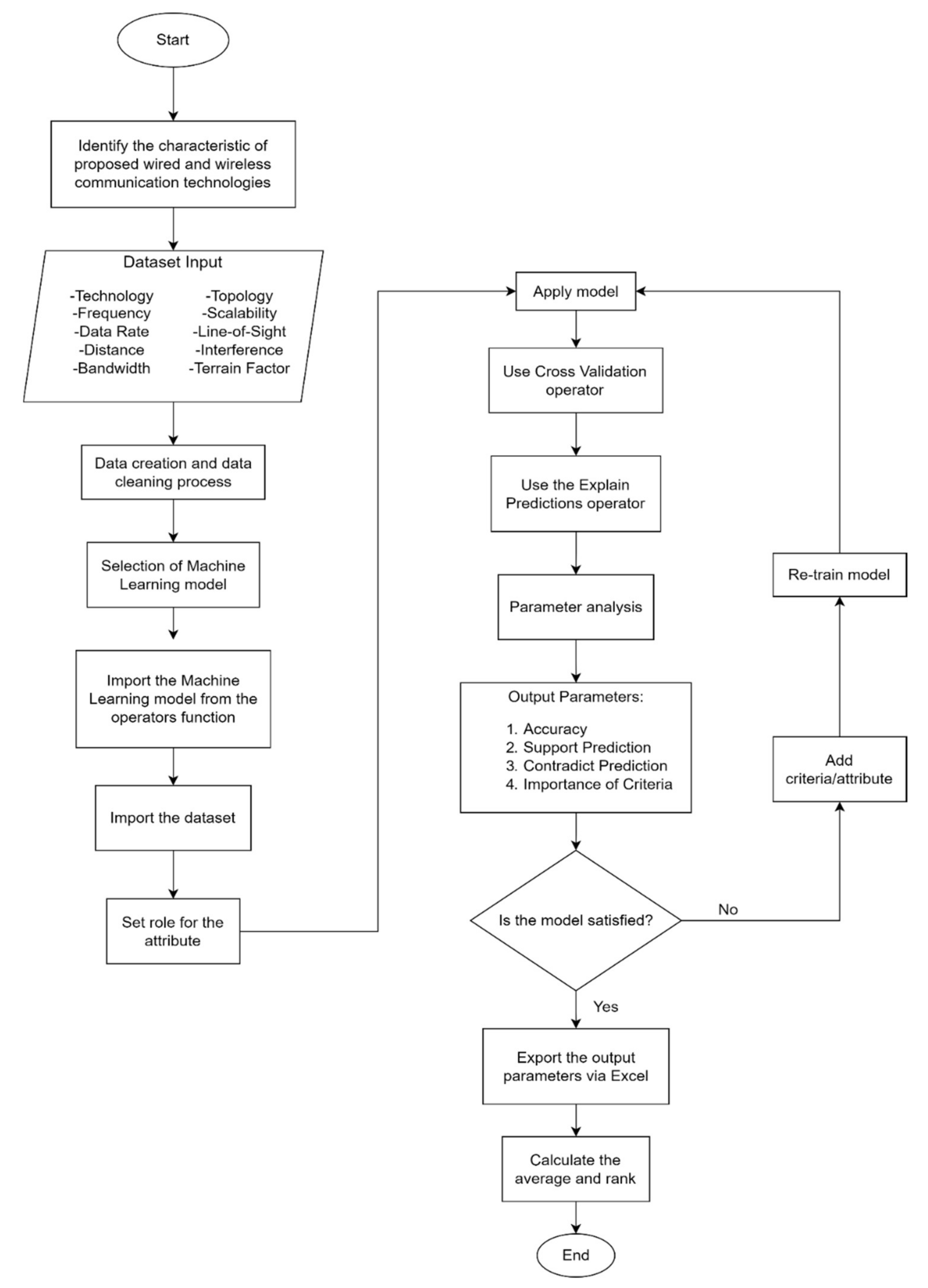
• A list of the potential communication technologies to be applied at the electrical distribution substation, based on extensive literature review.
• The creation of an ML dataset of the potential communication technologies based on the specifications in the literature.
• A thorough investigation on the ML models with the highest performance in selecting the most important criteria for electrical distribution substation communication technology.
• A ranking of the criteria from the most important to the least important, and an evaluation of the criteria that most strongly influence the selection of the best communication technology for the electrical distribution substation.

The remainder of the paper is structured as follows. Section 2 describes the communication technologies in detail, and Section 3 discusses the criteria and dataset specification for the ML model. Section 4 discusses the ML process and the preliminary results. The acronym used in the rest of this paper is tabulated in

Table 1. Acronyms and definition.

Acronyms	Definition
AMI	Advanced Metering Infrastructure
EV	Electric Vehicle
HAN	Home Area Network
IoT	Internet of Things
k-NN	k-Nearest Neighbor
LoS	Line of Sight
LTE	Long-Term Evolution
ML	Machine Learning
M2M	Multipoint-to-Multipoint
NB-IoT	Narrow-Band IoT
NBPLC	Narrowband Power Line Communication
P2M	Point-to-Multipoint
P2P	Point-to-Point
PLC	Power Line Communication
SATCOM	Satellite communication
UHF	Ultra-high frequency
WAN	Wide Area Networks

.

2. Selection of Communication Technology

The smart grid consists of three major components: electrical generation sources, transmission system, and distribution system, where communication plays an important role in providing reliable, efficient, and secure power transfer. The distribution system consists of all the facilities and equipment connecting a transmission system to the customer’s equipment and typically consists of distribution transformers, switches, distribution feeders, and substations [2]. The substation’s main function is to receive the energy transmitted from the generating station at high voltage, reduce it to an appropriate local distribution level, and provide switching facilities. This substation includes isolators, lightning arresters, step-down transformers, circuit breakers, and capacitor banks [3]. Communication systems allow information to be exchanged between monitoring systems, and data management systems, all of which necessitate fast and reliable communication. With the advent of distributed energy sources and energy storage systems closer to the consumer’s side, the importance of timely and dependable communication grows exponentially.

The initial step for this research starts with finding the potential communication technologies for the electrical distribution substations. The typical communication technologies for the smart grid consist of wired and wireless communication. Wired communication relies on a physical medium (cables) that exists between the transmitter and the receiver in a wired communication system, through which the signal is transferred. The cables can transmit and receive data depending on the capability of the cables themselves. Transmission of information over a distance without wires, cables, or any other electrical conductors is called wireless technology. The data transmission is transferred using electromagnetic waves such radio frequencies, infrared, and satellites.

In wired technology, power line communication (PLC) is widely used in smart grid applications, such as advanced metering infrastructure (AMI). PLC offers a wide range of technologies from the transmission grid to the distribution grid and home automation, such as ultra narrowband, narrowband, and broadband PLC [4]. Narrowband power line communication (NBPLC) is capable of handling and identifying equipment faults and is preferable on the distribution side of the power grid by participating in and supporting distributed generation (DG), microgrids, and consumer participation based on two-way communication [5].

Another wired communication technology that is commonly employed is fiber optics, which is used to provide backbone communication for various smart grid applications, such as substation automation and transmission domain communication, and to provide a long-term smart grid solution [6]. Fiber optics communication consists of several standards, such as AON (IEEE 802.3ah), BPON (ITU-T G.983), GPON (ITU-T G.984), and EPON (IEEE 802.3ah). Each standard possesses a different data rate and distance it can cover [7]. The distinction between PLC and fiber optics communication is that PLC communicates over existing electrical lines, whereas optical fiber communication involves the installation of fiber optics cables. It offers high bandwidth, low attenuation, small interference, and enhanced signal to noise ratio (SNR), making it a commonly utilised cable communications technology in the smart grid [8]. Despite the advantages, the most significant drawback of fiber optics communication is its high cost of installation. Furthermore, because the installation of fiber optic cables involves a significant amount of time, they are not ideal for quick deployment. Connecting geographical regions located in rocky or steep terrain is also difficult [8].

Zigbee is a wireless technology built on the IEEE standard 802.15.4 that is widely used in wireless communication for home or building automation, energy monitoring, managing industrial plants, as well as AMI applications [5]. As a result of its low power consumption and low deployment cost, it has been widely used in many smart grid applications in distributed automation, control, monitoring, management, and fault identification. Zigbee operates in unlicensed industrial, scientific, and medical (ISM) bands. However, since it shares the same spectrum with other wireless communication mediums, it is most likely to suffer from interference between the mediums [9].

Cellular networks, one of the most rapidly growing communication technologies, is also considered. This technology has rapidly evolved, starting from the 2G, 3G, 4G; the most recent is 5G technology. These cellular networks, particularly 4G, LTE, and 5G, provide numerous wide-area services to smart grid applications at a low cost [5]. For example, cellular networks can enable smart metering deployments in a wide area environment [6]. In addition, because of the existing network, the cellular network is ideal for rapid rollout. This technology is being used for AMI, home area network (HAN), wide area networks (WAN), and vehicle-to-vehicle (V2V) communication, among other applications [8]. Some of the features of cellular networks are that they offer high data rates, large coverage, high reliability and flexibility, and operate in both licensed and unlicensed spectrum. However, because the cellular system is shared by many users, it cannot support mission-critical applications that require uninterrupted service [8]. For 5G, there are some concerns on security and privacy issues, apart from the expected high deployment cost. Additionally, the long-term environmental impacts of 5G are still unknown. Because of their stability and capabilities, only 4G, 5G, and private long-term evolution (LTE) are considered in this research Furthermore, 1G, 2G, and 3G technologies are not included because they are considered sunset technologies and are no longer available in most parts of the world.

WiFi is a wireless network that is based on the IEEE 802.11 family of standards. In the IEEE 802.11 family, there are other standards, such as 802.11a, 802.11b, 802.11g (also known as enhanced WiFi), 802.11n (WiFi 4), 802.11ac (WiFi 5) and 802.11ax (WiFi 6). Each of the standards differs in terms of speed and the frequency band used. Some of the standards only utilise 2.4 GHz or 5 GHz, and some can utilise both frequencies. WiFi is mostly used in gadgets that utilise HAN technology, such as mobile phones, laptops, and personal computers [10]. From the research in [11], WiFi wireless sensor networks offer more advantages than Zigbee, such as large coverage, high bandwidth, cost effective, and ease of expansion. It also offers the advantage of high data rates, IP support, wide availability, and scalability [10]. However, the big challenges in using Wi-Fi for smart grid HAN applications are the interference between other wireless mediums and security issues.

LoRa (short for long range) is a wireless technology that provides long-distance, low-power, and secure data transfer for machine-to-machine (M2M) and internet of things (IoT) applications. It uses chirp spread spectrum (CSS)-derived modulation technology that uses lower power, such frequency-shift keying (FSK) modulation, for long-range communications. LoRa is a representation of low-power wide-area network (LPWAN) technology that operates in several ISM bands. Due to LoRa’s low data rate, it is only suitable for applications with small payloads, such as sensors and actuators that operate in low power mode, and is unsuitable for mission-critical services [9,12].

Another wireless communication that operates on the existing cellular networks, particularly the LTE facilities, is the narrow-band IoT (NB-IoT). The NB-IoT is capable of coexisting seamlessly with traditional GSM, general packet radio service (GPRS), and LTE technologies [9]. It offers an excellent battery life of 8 to 10 years, low channel bandwidth, a huge coverage area, is inexpensive, and possesses a good level of network security [12]. The NB-IoT can offer greater quality of service (QoS) compared with unlicensed technologies for neighbourhood area networks (NANs) and dependable services for mission-critical grid applications, such as meter reading and home automation [9]. However, NB-IoT is a latency-insensitive technology, which makes it more applicable to those delay-tolerant applications, such as AMI services.

Ultra-high frequency (UHF) is one of the wireless communication technologies that can be considered for electrical distribution substation communication. UHF is well-suited for applications that require only a small amount of bandwidth, such as monitoring or automation through the IEC 60870-5-104 protocol. Applications with modest data rate requirements and widely distributed end points, such as an extensive private broadband wireless infrastructure, may have a negative benefit-cost ratio. In these cases, newly upgraded UHF radio systems are a better fit for these requirements [13]. A major advantage of these UHF systems is their ability to scale dynamically between throughput and range. They are also suitable for mission-critical applications due to the deployment of licensed spectrum and the flexibility of private network architecture [13].

The RF mesh is a standard adopted by the Wireless Smart Utility Networks Alliance (Wi-SUN Alliance). It is for building private wireless networks based on a mesh topology, with each network node acting as a repeater. As a result, each element can be accessed directly by an access point or indirectly via another network terminal element over one or more hops [14]. In order to assure compatibility across networks and devices from different manufacturers, RF Mesh aspires to be a system built on open standards. For utility applications, RF Mesh is a well-established and practical technology. From a technological and functional standpoint, RF Mesh was designed to satisfy the requirements of critical utility applications, such as smart metering and distribution automation in the case of the electric sector [14].

Satellite communication, often known as SATCOM, is a technology that has been extensively utilised for a variety of purposes, including direct-to-home (DTH), geological monitoring, and military uses. SATCOM consists of several frequency bands such as C-band, L-band, X-band, Ku-band, and Ka-band. Due to the system’s location in space, natural calamities, such as floods and earthquakes, do not effect this system, making it one of the advantages [8]. SATCOM also offers a high availability range and is suitable for deployment in areas lacking terrestrial communication facilities, as the facilities are either expensive or insufficient for domain needs [15]. The disadvantage is that data transmission will be delayed due to the great distance between the earth and the satellite system, making it unsuitable for real-time monitoring and control applications [8].

3. Criteria and Dataset Specification

Each of the shortlisted technologies in Section 2 has numerous characteristics and technical criteria that may need to be considered when selecting a communication solution for the substation. Due to this, ML was employed to help in the selection of criteria that are important in deciding or selecting the best communication technology for the substations. The ML process needs a dataset to train on in order to make the right selection. This dataset must be comprehensive and cover all of the criteria for the communication technologies suitable for implementation at the electrical distribution substation. The identified criteria were frequency, data rate, distance, bandwidth, line of sight (LoS), scalability, interference, topology, and terrain factor (city, plains, coastal, forestry, and mountains). The overall flow of this research is summarized in Figure 1. The information below is the justification of the selected criteria:

• Frequency is defined as the rate of radio signals measured in Hertz (Hz) to transmit and receive communication signals. Each technology has its own operating frequency spectrum, which can be classified into two categories: (1) licensed: assigned solely to operators for independent use; and (2) unlicensed: assigned to each citizen for non-exclusive use subject to regulatory limits such as transmission power restrictions.
• Bandwidth is defined as the range that carries a signal within a band of frequencies. For example, a system that operates on frequencies between 150 MHz and 200 MHz operates with a bandwidth of 50 MHz.
• Data rate is defined as the amount of data transmitted over a network in a certain period of time, commonly expressed in megabit per second (Mbps).
• Distance refers to the coverage offered by a communication technology. Some wireless technologies, such as SATCOM, LoRa, and private LTE, are known to offer long-distance coverage, whereas others offer short-distance coverage (Zigbee, WiFi). Shorter coverage usually leads to higher deployment of a particular technology in the selected areas.
• Terrain factor divides the land into several categories as follows:

  (a)

  City: The city area is known to contain the highest user density, with buildings and existing wireless communication technologies. It is one of the factors affecting the reliability of communication technologies, especially in terms of the line-of-sight (LoS) interference.

  (b)

  Coastal: The coastal area is defined as the interface or transition area between land and sea, including large inland lakes. Because of its large area and low population density, it is assumed to contain no LoS interference.

  (c)

  Plains: The plains are defined as a broad area of relatively flat land. The assumption is that they contain lower user density compared to the city and less or almost no LoS interference due to the wide area and lower vegetation.

  (d)

  Forestry: A forest is defined as an area with more than 0.5 hectares of land, trees taller than 5 m, and a canopy cover of more than 10%, or trees capable of reaching these thresholds in situ. It does not include land that is predominantly used for agricultural or urban land use. The assumption is that it contains the lowest user density. However, the high density of forest affects the communication technology’s reliability, especially for wireless technology.

  (e)

  Mountains: A mountain is a land that is raised above the surrounding landscape. It is usually in the form of a peak with a well-defined summit. The assumption is that mountainous areas contain low density of users and trees. However, due to the topography, it requires higher cost and longer time for cable installation.

• Scalability is defined in this research as the ability of the communication technology to be scaled, measured in terms of percentage. It is dependent on the topology and data rate that each technology can offer, in which the more devices are added to a network, the longer the communication delay on the network. This means that the number of devices added to a network topology needs to be monitored carefully to make sure that the network resources are not stretched beyond their limit. Point-to-point (P2P) topology is not scalable, whereas point-to-multipoint (P2M) and multipoint-to-multipoint (M2M) are considered scalable. The ring topology raises scalability concerns, as the bandwidth is shared by all devices within the network. A star and mesh topology network is considered scalable, as network nodes can be added with minimal disruption.
• Line-of-Sight (LoS) interference, measured in terms of percentage in this research, refers to the setting when the transmit and receive nodes are not in view of each other due to the presence of obstacles between them. A higher percentage is given to the wired technologies than to the wireless technologies due to the latter’s reliability against LoS interference. The reliability of wireless technology is lower than wired technology, taking into consideration the example of Urban (City): high density with buildings, Suburban (Coastal and Plains): higher than Urban and Rural because there are no or few LOS interferences due to the wide area and lower density (buildings, trees), Rural (Forestry): high density of trees and Rural (Mountains): slightly lower considering lower density of trees.
• Interference refers to spectrum interference, measured in percentage in this research. For wired technology, the assumption is that the interference is lower than the wireless technology. To the best of our knowledge, wired technology’s only source of interference is interference from other mediums. Additionally, it is expected that there will be less interference in wired technologies as they are mostly buried underground. The terrain factor affects interference in wireless technology, especially because of the user density in a particular area. For example, in urban areas (cities), the interference is expected to be the highest compared to other areas due to the high density of users.

The process for ML dataset creation starts with identifying the technical criteria of the proposed wired and wireless communication technologies, a visualization of the created dataset is shown in

Table 2. The visualization of the training dataset in Microsoft Excel.

Technology	Frequency (MHz)	Data Rate (Mbps)	Distance (km)	Frequency Bandwidth (MHz)	Physical Topology	Scalability (%)	Line-of-Sight (%)	Interference (%)	Terrain Factor
NBPLC	0.01	0.5	150	0.1	Point-to-Point	30	70	60	City
NBPLC	0.01	0.5	150	0.1	Point-to-Multipoint	45	70	60	City
NBPLC	0.1	0.5	150	0.1	Point-to-Point	30	70	60	City
NBPLC	0.1	0.5	150	0.1	Point-to-Multipoint	45	70	60	City
NBPLC	0.3	0.5	150	0.1	Point-to-Point	30	70	60	City
NBPLC	0.3	0.5	150	0.1	Point-to-Multipoint	45	70	60	City
NBPLC	0.5	0.5	150	0.1	Point-to-Point	30	70	60	City
NBPLC	0.5	0.5	150	0.1	Point-to-Multipoint	45	70	60	City
Fiber	193,000,000	1000	70	50,000	Point-to-Point	60	85	60	City
Fiber	193,000,000	1000	70	50,000	Point-to-Multipoint	80	85	60	City
Fiber	193,000,000	1000	70	100,000	Point-to-Point	60	85	60	City
Fiber	193,000,000	1000	70	100,000	Point-to-Multipoint	80	85	60	City
NBPLC	0.01	0.5	150	0.1	Point-to-Point	30	70	45	Coastal
NBPLC	0.01	0.5	150	0.1	Point-to-Multipoint	45	70	45	Coastal

.

These technical criteria were chosen from various literature reviews [4,5,6,7,8,9,10,11,12,13,14,15] and surveys that are related to the possible communication technologies and were summarised in

Table 3. The criteria specification of selected communication technologies.

Technology	Frequency (MHz)	Data Rate (Mbps)	Distance (km)	Frequency Bandwidth (MHz)	Physical Topology	Terrain Factor	Scalability(%)	LoS (%)	Interference(%)
NBPLC	0.01 0.1 0.3 0.5 [5,16,17]	0.5 [5,6] [16,18]	150 [6,18]	0.1	P2P P2M [5,19]	City Coastal Plains Forestry Mountains	City: 30 (P2P), 45 (P2M) Coastal and Plains: 30 (P2P), 45 (P2M) Forestry and Mountains: 25 (P2P), 40 (P2M)	City: 70 Coastal and Plains: 70 Forestry: 70 Mountains: 60	City: 60 Coastal and Plains: 45 Forestry: 40 Mountains: 35
Fiber optics	193,000,000 [20]	1000 [21]	70 [21]	50,000 100,000	P2P P2M [6,22]	City Coastal Plains Forestry Mountains	City: 60 (P2P), 80 (P2M) Coastal and Plains: 60 (P2P), 80 (P2M) Forestry and Mountains: 55 (P2P), 75 (P2M)	City: 85 Coastal and Plains: 85 Forestry: 85 Mountains: 75	City: 60 Coastal and Plains: 45 Forestry: 40 Mountains: 35
Zigbee	2400 [5,6,10] [16,17] [22,23,24,25]	0.25 [5,6,10] [17,23,24,25,26,27]	0.07 [5,6,10] [23,24,26]	2 [25]	P2P Star P2M Mesh [5,10,16,22] [24,27,28]	City Coastal Plains Forestry Mountains	City: 35 (P2P), 55 (Star), 55 (P2M), 70 (Mesh) Coastal and Plains: 35 (P2P), 55(Star), 55 (P2M), 70 (Mesh) Forestry and Mountains: 30 (P2P), 50 (Star), 50 (P2M), 65 (Mesh)	City: 60 Coastal and Plains: 60 Forestry: 60 Mountains: 50	City: 75 Coastal and Plains: 60 Forestry: 55 Mountains: 50
WiFi	2400 5000 [6,10,16] [23,24] [26,28,29]	150 450 [5,6,10,18] [27,30]	0.125 0.07 [5,29,30]	20 22 26 [30]	P2P P2M Star Mesh [26,28,31]	City Coastal Plains Forestry Mountains	City: 45 (P2P), 65 (P2M), 65 (Star), 80 (Mesh) Coastal and Plains: 45 (P2P), 65 (P2M), 65 (Star), 80 (Mesh) Forestry and Mountains: 40 (P2P), 60 (P2M), 60 (Star), 75 (Mesh)	City: 60 Coastal and Plains: 60 Forestry: 60 Mountains: 50	City: 75 Coastal and Plains: 60 Forestry: 55 Mountains: 50
RF Mesh	2400	0.1 [14,32]	5 (Urban), 8 (Suburban), 12 (Rural) [14,32]	0.2 0.7 1.2	Mesh [32]	City Coastal Plains Forestry Mountains	City: 70 Coastal and Plains: 70 Forestry and Mountains: 65	City: 60 Coastal and Plains: 60 Forestry: 60 Mountains: 50	City: 75 Coastal and Plains: 60 Forestry: 55 Mountains: 50
Cellular Network—4G LTE	900 1800 2600 [33,34]	100 [24]	2 (Urban), 3 (Suburban), 6 (Rural) 1.42 (Urban), 2.44 (Suburban), 5.88 (Rural) 1 (Urban), 2.05 (Suburban), 4.09 (Rural)	20	P2P [26,28,35]	City Coastal Plains Forestry Mountains	City: 45 (P2P) Coastal and Plains: 45 (P2P) Forestry and Mountains: 40 (P2P)	City: 60 Coastal and Plains: 60 Forestry: 60 Mountains: 50	City: 75 Coastal and Plains: 60 Forestry: 55 Mountains: 50
5G	700 3500 26,000 28,000 [36]	100 to 20,000 [37]	10 to 100 [38]	1000 [39,40]	P2P [41]	City	City: 50 (P2P)	City: 50	City: 75
Cellular Network—Private LTE	450 900 2300	0.256, 0.512, 1.024 100	450 MHz: - 30 (Urban, Suburban, Rural) 900 MHz: - 2 (Urban), - 3 (Suburban), - 6 (Rural) 2300 MHz: - 2 (Urban, Suburban, Rural) [42]	10 20 5	P2P M2M Mesh [26,28,35]	City Coastal Plains Forestry Mountains	City: - 450 MHz: 35 (P2P), 55 (M2M), 70 (Mesh) - 900 MHz: 45 (P2P), 65 (M2M), 80 (Mesh) - 2300 MHz: 35 (P2P), 55 (M2M), 70 (Mesh) Coastal and Plains: - 450 MHz: 35 (P2P), 55 (M2M), 70 (Mesh) - 900 MHz: 45 (P2P), 65 (M2M), 80 (Mesh) - 2300 MHz: 35 (P2P), 55 (M2M), 70 (Mesh) Forestry and Mountains: - 450 MHz: 30 (P2P), 50 (M2M), 65 (Mesh) - 900 MHz: 40 (P2P), 60 (M2M), 75 (Mesh) - 2300 MHz: 30 (P2P), 50 (M2M), 65 (Mesh)	City: 60 Coastal and Plains: 60 Forestry: 60 Mountains: 50	City: 60 Coastal and Plains: 45 Forestry: 40 Mountains: 35
NB-IoT (LTE)	900 1800 2600 [34,43]	0.2 [43]	1 (Urban), 5 (Suburban), 10 (Rural) [43]	0.2 [43]	P2P P2M Star [43]	City Coastal Plains Forestry Mountains	City: 45 (P2P), 55 (P2M), 55 (Star) Coastal and Plains: 45 (P2P), 55 (P2M), 55 (Star) Forestry and Mountains: 40 (P2P), 50 (P2M), 50 (Star)	City: 60 Coastal and Plains: 60 Forestry: 60 Mountains: 50	City: 75 Coastal and Plains: 60 Forestry: 55 Mountains: 50
LoRa	433 [43,44,45]	0.0055 0.022 [45]	5 (Urban), 15 (Suburban), 20 (Rural) [43]	0.125 0.5 [45,46]	Star Mesh [47]	City Coastal Plains Forestry	City: 55 (Star), 70 (Mesh) Coastal and Plains: 55 (Star), 70 (Mesh) Forestry and Mountains: 50 (Star), 65 (Mesh)	City: 60 Coastal and Plains: 60 Forestry: 60 Mountains: 50	City: 75 Coastal and Plains: 60 Forestry: 55 Mountains: 50
SATCOM	C band: 4–8 GHz [15,48]	0.032	100–6000	0.1	Star Mesh	Coastal Plains Mountains	Coastal and Plains: 55 (Star), 70 (Mesh) Mountains: 50 (Star), 65 (Mesh)	Coastal and Plains: 60 Mountains: 50	Coastal and Plains: 60 Mountains: 50
UHF	450–470 [49]	0.032 0.064 [49]	30	0.0125 0.025 [49]	P2P P2M [50]	Coastal Plains Mountains	Coastal and Plains: 35 (P2P), 55 (P2M) Mountains: 30 (P2P), 50 (P2M)	Coastal and Plains: 60 Mountains: 50	Coastal and Plains: 45 Mountains: 35

. These criteria are deemed to be crucial and fit with the purpose of this study. Each criterion was chosen based on the applicability, the general usage and how can it be implemented in various areas, such as urban, suburban and rural. Each criterion has different characteristics, for example, for distance, each area has different length of coverage. All of these factors were considered and examined to ensure that the data creation process was smooth, simple and straightforward.

From the criteria summarized in the Table 3, a total of 880 lines of communication technology data were created using Microsoft Excel. This dataset served as a training input for the ML models in the RapidMiner software, in which the performance of each ML model was evaluated and analysed. The next section will describe how the dataset was processed using the RapidMiner software.

4. Machine Learning (ML)

ML has been widely used in various applications and fields. Nowadays, data can be obtained across the internet, but the method of extracting or obtaining knowledge from the data can be very challenging. With the aid of ML, the learning process of the data can be performed with minimal calculation and less time consumption. The continuous learning process is needed to ensure continuous development. In practice, this means enabling a model to learn and adapt autonomously in production as new data is received. ML is described as a computer’s capacity to learn and improve its accuracy over time without being instructed to do so. In ML, an algorithm has been trained several times to adapt and detect patterns in order to be able to make decisions and pre-dictions based on newly acquired information [51]. Better algorithms often result in more accurate decisions and predictions. Some of the ways to choose an algorithm is by looking at the size of the training data, accuracy and/or interpretability of the out-put, the training time, and the number of features. ML can be classified into three different categories, namely, supervised ML, unsupervised ML, and reinforcement and semi-supervised learning [52,53].

In this research, supervised ML was selected as it has the capability of predicting continuous quantities (regression) and predicting a label or class (classification). In particular, supervised ML will be used for the identification of the communication technology class based on the technical criteria dataset. This will consequently lead to the identification of the technical criteria having the biggest contribution to the decision on choosing the best communication technologies for the electrical distribution substation. To the best of our knowledge, there are limited studies related to criteria selection via ML especially in the communication technology field. An example of ML criteria selection in a different field can be found in [54], in which in the authors per-formed criteria selection in the selection of non-native language Master of Business Administration (MBA) students in Shanghai International MBA Program in China. Some of the major criteria of the study includes age, oral English fluency, and working years. The authors evaluated three different ML approaches: Ridge Linear Regression, Gradient-Boosted Decision Trees (GBDT), Random Forests and SVM. Each of these algorithms is subjected to tenfold cross validation, which is similar to our method.

Figure 2 depicts the steps of the ML modelling used, with each block representing an operator that was used in the modelling. The created dataset in Section 3 was imported into RapidMiner, and was applied to several ML models specialising in the classification method, such as naïve Bayes, decision tree, random forests, k-nearest neighbours (k-NN), and gradient boosted trees. These ML approaches were chosen and shortlisted for this study because they are considered to be among the most well-known approaches in the field of supervised machine learning. Other ML approaches such as support vector machine (SVM), artificial neural networks, logistic regression and perceptron, were not selected, as RapidMiner had identified them not suitable based on the dataset. This is because the label data was in polynomial instead of binomial or real or integer. These ML models could not identify the polynomial data, making them unsuitable to be used. RapidMiner is used for this project since it has become one of the most popular tools for the ML models due to its graphical user interface, and because it is user friendly and easy to use compared to other code-based software. The tools and functions provided by RapidMiner are efficient for data observation, comparison, results evaluation, and analysis. It also offers extensive documentation, numerous worked examples, training, and support from a large user community. A brief description on these ML models are as follows, while the advantages and disadvantages of these ML models are described in

Table 4. The advantages and disadvantages of the selected ML models.

ML Model	Advantages	Disadvantages
Naïve Bayes	Time-efficient. Suitable for solving multi-class prediction problems Better performance and requires fewer training data than other models if its assumption of the independence of features holds true. Better suited for categorical input variables than numerical variables.	Limited applicability in real-world use cases due to its assumption that all predictors/features are independent, which rarely happens in real life. Smoothing technique is needed to solve the ‘zero-frequency problem’ where it assigns zero probability to a categorical variable whose category in the test dataset was unavailable in the training dataset. Its probability output estimations are not precise in some cases.
Decision Tree	Easy to use and understand. Can handle both categorical and numerical data. Resistant to outliers, hence, require little data pre-processing. New features can be easily added. Can be used to build larger classifiers by using ensemble methods.	Prone to overfitting. Require some kind of measurement as to how well they are doing. Need to be careful with parameter tuning. Can create biased learned trees if some classes dominate.
Random Tree Forest	Reduces overfitting in decision trees and helps to improve the accuracy. It is flexible to both classification and regression problems. It works well with both categorical and continuous values, and it automates missing values in data. Normalizing of data is not required as it uses a rule-based approach.	It requires large computational power as well as resources as it builds numerous trees to combine their outputs. It takes a long time to train because it combines many decision trees to determine the class. It also lacks interpretability due to the ensemble of decision trees and fails to determine the significance of each variable.
Gradient Boosted Tree	Is generally more accurate compared to other models. It trains faster especially on larger datasets. It provides support for handling categorical features. Able to handle missing values natively.	Prone to overfitting. It can be computationally expensive and take a long time to train, especially on central processing units (CPUs). It can be hard to interpret the final models.
k-Nearest Neighbor	Quick calculation time. Simple algorithm. Versatile and useful for regression and classification. High accuracy. It does not require any data assumptions. As a result, there is no need to make additional assumptions, fine-tune several parameters, or construct a model. This is especially important in the case of non-linear data.	Accuracy depends on the quality of the data. With large data, the prediction stage might be slow. Sensitive to the scale of the data and irrelevant features. Require high memory, needs to store all of the training data. Given that it stores all of the training, it can be computationally expensive.

.

Naïve Bayes: The Naïve Bayes method is a form of supervised learning that is based on the Bayes’ theorem, which involves conditional probability and is used to solve classification problems. A Naïve Bayes classifier assumes that the presence of one feature in a class has no relationship with the presence of any other feature [53]. The overall structure of Naïve Bayes is called the Bayesian network. Naive Bayes is described as a method of classification that requires only a small amount of training data. Another advantage is that it has a short computational time for training [53,55].

Decision Tree: The decision tree is another supervised ML model used for classification. Essentially, it is a basic tree that contains of branches where each branch indicates a possible value a node may have and nodes, where the node represents attributes of a group that is to be classified [53,55]. The tree structure is simple to comprehend and gives a clear perspective for decision-making. But it has several disadvantages, such as overfitting, and errors due to bias and variance. A simple technique to avoid overfitting is to pre-prune the decision tree by preventing it from growing to its maximum size [55].

Random Tree Forest: The Random Tree Forest is an improvement on the Decision Tree, which is a versatile and powerful ensemble classifier [56]. It has the capability of generating a huge number of trees using random bootstrapped samples of the training dataset. Random Forests need two parameters to be tuned, including the number of trees (ntree), and the number of variables (mtry) [56]. However, since this method generates a huge number of trees, the process consumes more time than the Decision Tree and takes more effort to comprehend and evaluate. This is because each tree in the forest will be produced, processed, evaluated, and analysed individually [57].

Gradient Boosted Tree: The gradient boosted tree is an ensemble of either regression or classification tree models [58]. Its ensemble of weak prediction models usually involves a decision tree to produce an improved or strong prediction model. Gradient boosted trees function by building each succeeding tree consecutively and learning from the faults of the preceding tree. The process of identifying and updating the pattern is then repeated until no pattern can be modelled and the sum of residuals approaches zero and the predicted values approach the actual values [59].

k-Nearest Neighbor (k-NN): The k-NN is a simple but effective supervised ML algorithm [60]. This approach provides a class label to an unlabeled item based on the class labels of its k nearest neighbours. The model is simple to implement, robust to noisy training data, and effective even with large amounts of training data.

The steps of ML modelling start with importing the training dataset into the RapidMiner software, using the ‘Retrieve’ operator. Next, the ‘Set Role’ operators are used to assign a class to an attribute. In this case, the technology criteria were set as a label role. A label role works as a learning operator target attribute and is often referred to as ‘target variable’ or ‘class’. After assigning a role to the imported dataset, the information was fed into the ‘Cross Validation’ operator. Each ML approaches uses default parameters for both variables and hyperparameters. Thus, no optimization is required.

Cross-validation is one of several data resampling methods, including randomization, bootstrap, and jackknife [61]. This method’s function is to estimate the accuracy and efficacy of an ML model [62,63], while [64] states that the overall goal of cross validation is to assess the generalization ability of predictive models and to avoid overfitting. This method will randomly split the data by dividing into one or more subsets for resampling. The ‘Cross Validation’ operator, in particular, is divided into two sub-processes: training and testing. Each of the ML models will undergo the training sub-process before being applied in the testing sub-process. The performance obtained during the testing phase is used as an accuracy marker for the ML model, with accuracy defined as how accurate the model is in determining the labelled data, and it is calculated by dividing the percentage of correct predictions by the total number of examples. As mentioned in [65], the authors stated that the cross-validation method aided in these three ways:

• It reduced the variability in prediction errors.
• It made the best use of all available data while avoiding overfitting or overlap between test and validation data.
• It avoided testing hypotheses provided by arbitrarily split data.

Some of the cross-validations variants are K-fold cross validation, leave-one-out cross-validation, stratified K-fold cross-validation, Repeated K-fold cross-validation, nested cross-validation, and time series cross-validation [66,67]. In this research, the K- fold cross validation was selected. The K-fold technique is popular and simple to grasp; it produces a less biased model when compared to other methods because it assures that every observation in the original dataset holds a chance of appearing in both the training and test sets and suitable for limited input data. Moreover, one option for improving the holdout method is to use K-fold cross validation. This strategy ensures that the ML model’s score is independent of how we chose the train and test sets [63,68].

The general procedures of K-fold cross validation are as follows [69,70]:

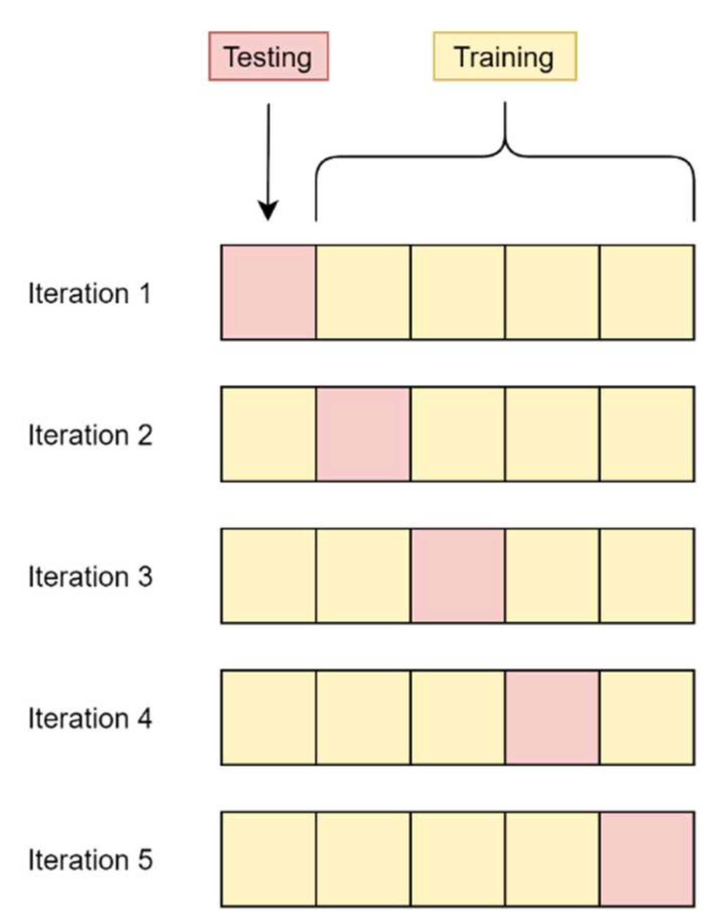
• Pick any number of folds, K. Ideally, it can be from 5 to 10, depending on data sizes.
• The dataset will be divided into K equal subsets, which are also called folds.
• Choose K − 1 folds, which will be the training set. The remaining folds will be the test set.
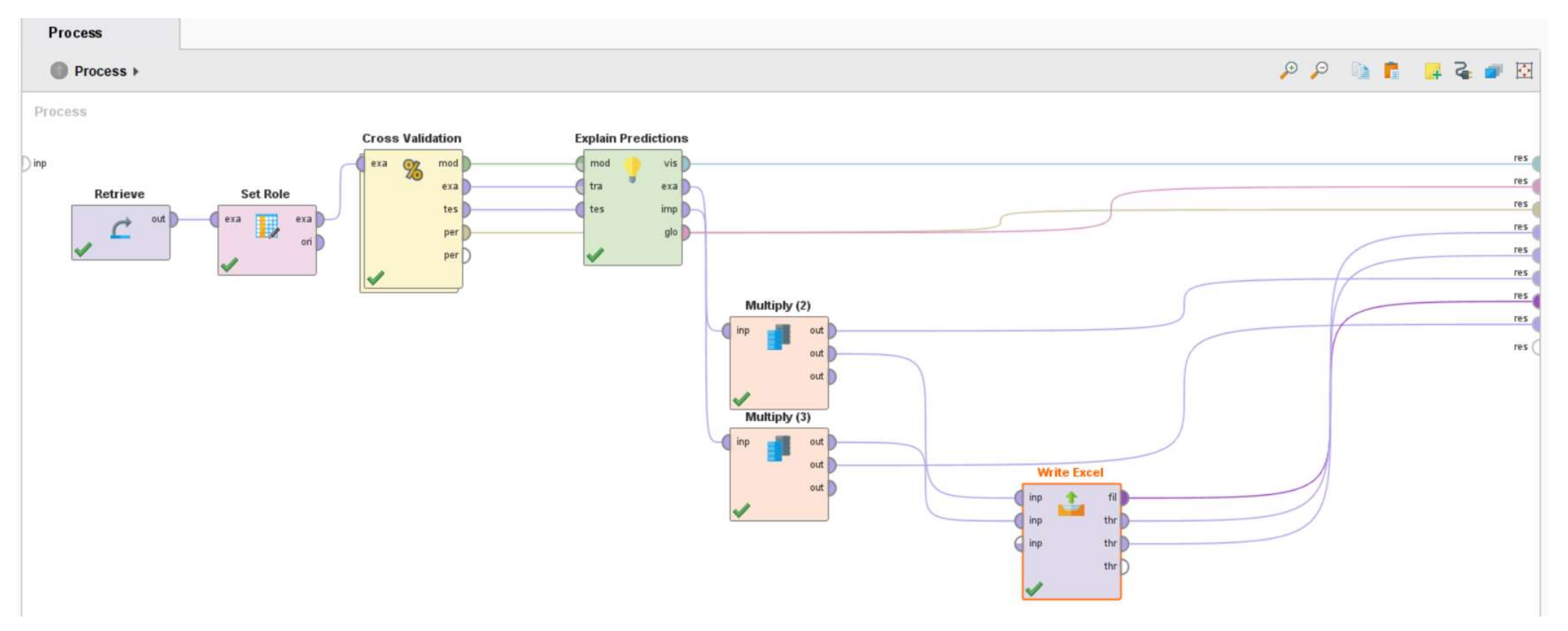
• Use the cross-validation method to train the ML model and calculate its accuracy
• Evaluate the accuracy using all the K cases of cross validation.

Figure 3 shows an example when the number of folds is equal to 5, which also summarizes the general procedure for conducting the K-fold cross validation. Typically, a number of K = 10 is used in a vast area [65,71]. As K increases, the size of the gap between the training set and the resampling subset decreases. Consequently, the technique’s bias decreases (i.e., the bias is less for K = 10 than it is for K = 5), in which the bias defined in this context is the difference between estimated and true performance values [72].

The authors in [71] proposed a repeated cross validation with K = 10, especially for the research problems that are often encountered in the social sciences. Cross validation is also used to predict fatty liver disease, with the authors using k-fold cross validation on several machine learning algorithms [65]. They proposed four different machine learning algorithms: Random forest, naïve Bayes, artificial neural networks, and logistic regression, each with three different K values (3, 5, 10). Observation shows that the random forest performed best with K = 10. As a result, K = 10 was also used in our analysis. As stated in [70], because training and testing are done on separate sections of the dataset, the K-fold produces a more consistent and trustworthy result. It is also possible to improve the overall score by increasing the number of folds used to test the model on a variety of different sub-datasets. The disadvantage is that increasing the number of K in training more models may lengthen the training process.

The output of the ‘Cross-validation’ operator is then fed into the ‘Explain Prediction’ operator to find the ML model’s performance using the ‘support prediction’, and the ‘contradict prediction’ values. The ‘Explain Prediction’ operator provides statistical and visual observations to help understand the role of each attribute/criterion on the prediction. Essentially, this operator will create a table highlighting the attributes that most strongly support or contradict each prediction. Additionally, the table is also presented with two additional columns providing numeric data values on the support and contradict predictions [73]. This operator works with all data types and data sizes. It supports both classification and regression problems. The only ML model type that is not recommended is random forest, since this model typically suffers from long runtimes. The output from both the ‘Cross Validation’ and ‘Explain Prediction’ operators are exported into an Excel file via the ‘Write Excel’ operator for further analysis on the outcome.

5. Results and Discussion

The obtained results from the ‘Cross Validation’ and ‘Explain Prediction’ operators are tabulated in

Table 5. Results comparisons obtained from the RapidMiner simulation.

Models	Cross Validation Accuracy	Standard Deviation	Execution Time (Cross Validation)	Execution Time (Explain Prediction)
Naïve Bayes	98.41%	+/− 0.79%	28–50 ms	3320–3800 ms
Decision Tree	97.05%	+/− 2.94%	45–80 ms	1800–2500 ms
Random Forest	97.95%	+/− 1.29%	980–2400 ms	144,000–160,000 ms
Gradient Boosted Tree	98.07%	+/− 1.52%	3700–9400 ms	28,000–40,000 ms
k-NN	97.73%	+/− 1.42%	95–150 ms	47,000–55,000 ms

, which shows the comparison between each ML model in terms of accuracy, standard deviation, classification error, the cross-validation execution time, and ‘Explained Prediction’ execution time when K = 10. The model with the highest accuracy is then selected for the elimination of the least important criteria for the electrical distribution substation communication technology. The output of the ‘Explain Prediction’ operator for the chosen ML model was specifically evaluated in terms of its supporting and contradicting prediction values. Following that, an average value for each technical criterion was calculated, and the criteria were ranked in order of importance, as shown in

Table 6. Ranked technical criteria based on the average values of the output of the ‘Explain Prediction’ operator.

Criteria	Average
Frequency	0.0127919
Distance	0.0086610
Scalability	0.0048568
Data rate	0.0037547
Reliability	0.0032249
Physical Topology	0.0013349
Frequency Bandwidth	0.0003337
Terrain Factor	−0.0016518
Interference	−0.0067775

.

From Table 5, it can be observed that the Naïve Bayes model showed the highest accuracy, the lowest standard deviation, and the shortest cross validation execution time. Furthermore, the ‘Explain Prediction’ operator execution time was the second shortest of the five models tested. As this research only required a one-time process to determine which criteria should be prioritized, accuracy took precedence over time spent. Although the random forest model’s performance in cross-validation accuracy was comparable to naïve Bayes, with almost a 0.5% difference and a +/− 0.5% standard deviation, its execution times for both ‘Cross Validation’ and ‘Explain Prediction’ operators were longer. Additionally, the naïve Bayes model offered several advantages over the random forest model, in which its model size was low and quite constant with respect to the data [74]. Since naïve Bayes models cannot reflect complex actions, they would not overfit. On the other hand, the random forest model may result in overfitting if not carefully developed [74].

From its performance shown in Table 5, the naïve Bayes ML model was selected for further analysis. Specifically, the outcomes of the ‘Explain Prediction’ operator for naïve Bayes were used to assist in the elimination of the least important technical criteria for the electrical distribution substation communication technology. The output of the operator showed which technical criteria support or contradict the predictions. It also listed the importance of the technical criteria row by row with respect to the column, presented in numerical values. From that, an average was determined to assist in the ranking of the criteria, with the highest influence on the selection of the communication technology. Table 6 shows the average of the criteria for the 880 data points from the Naïve Bayes model. It can be observed that terrain factor and interference held the most negative attributes out of the nine criteria considered. These two lowest criteria shall be omitted because they are regarded as the least important and have no significant impact on the selection of electrical distribution substation communication technologies. The remaining seven technical criteria should be evaluated to determine the best communication technology solution for the electrical distribution substation.

6. Conclusions

This paper presents a method for technical criteria selection using ML for electrical distribution substation communication technology solution. Manually selecting an appropriate communication technology as a communication solution for an electrical distribution substation can be difficult, especially when numerous factors and criteria are involved. Thus, in this paper, ML was used to aid in the selection process by short-listing the numerous technical criteria of the potential communication technologies, based on the influences of each criterion on the communication technology selection. More specifically, this paper provided a list of the potential communication technologies to be applied at the electrical distribution substation, based on an extensive literature review. From the list provided, the technical criteria (or specifications) of each of the communication technologies were identified for the creation of the ML training dataset. This dataset was used for a supervised ML process in the RapidMiner software package, where a thorough investigation into the performance of several ML models in the classification of the communication technology criteria was conducted. From the investigation, the naïve Bayes model showed the highest overall performance in terms of accuracy and execution time. The output from the naïve Bayes’ analysis was then used to rank and eliminate the technical criteria that held negative attributes for the selection of communication technology for electrical distribution substation. The ranking of these criteria was expected to simplify the selection process of the best communication technology for the electrical distribution substation. As for future work, the remaining seven technical criteria will be evaluated further to determine the most suitable communication technology for the electrical distribution substation.

References

1. Li, R. Chapter 4—Protection and control technologies of connecting to the grid for distributed power resources. In Distributed Power Resources; Li, R., Ed.; Academic Press: Cambridge, MA, USA, 2019; pp. 121–144. [Google Scholar]
2. Transmission vs. Distribution. Available online: https://www.osha.gov/etools/electric-power/generation-transmission-distribution/transmission-distribution (accessed on 11 October 2021).
3. What Is a Substation—Definition, Types of SubStations. Available online: https://www.elprocus.com/what-is-a-substation-definition-types-of-substations/ (accessed on 11 October 2021).
4. Masood, B.; Baig, S. Standardization and deployment scenario of next generation NB-PLC technologies. Renew. Sustain. Energy Rev. 2016, 65, 1033–1047. [Google Scholar] [CrossRef]
5. Raza, N.; Akbar, M.Q.; Soofi, A.A.; Akbar, S. Study of Smart Grid Communication Network Architectures and Technologies. J. Comput. Commun. 2019, 7, 19–29. [Google Scholar] [CrossRef] [Green Version]
6. Kuzlu, M.; Pipattanasomporn, M. Assessment of communication technologies and network requirements for different smart grid applications. In Proceedings of the 2013 IEEE PES Innovative Smart Grid Technologies Conference, Washington, DC, USA, 24–27 February 2013; IEEE: Manhattan, NY, USA, 2013; pp. 1–6. [Google Scholar]
7. Kabalci, E.; Kabalci, Y. Introduction to Smart Grid Architecture. In Smart Grids and Their Communication Systems; Kabalci, E., Kabalci, Y., Eds.; Springer: Singapore, 2019; pp. 3–45. [Google Scholar]
8. Appasani, B.; Maddikara, J.B.R.; Mohanta, D.K. Standards and Communication Systems in Smart Grid. In Smart Grids and Their Communication Systems; Kabalci, E., Kabalci, Y., Eds.; Springer: Singapore, 2019; pp. 283–327. [Google Scholar]
9. Li, Y.; Cheng, X.; Cao, Y.; Wang, D.; Yang, L. Smart choice for the smart grid: Narrowband internet of things (NB-IoT). IEEE Internet Things J. 2018, 5, 1505–1515. [Google Scholar] [CrossRef]
10. Mahmood, A.; Javaid, N.; Razzaq, S. A review of wireless communications for smart grid. Renew. Sustain. Energy Rev. 2015, 41, 248–260. [Google Scholar] [CrossRef]
11. Li, L.; Hu, X.; Chen, K.; He, K. The applications of WiFi-based Wireless Sensor Network in Internet of Things and Smart Grid. In Proceedings of the 2011 6th IEEE Conference on Industrial Electronics and Applications, Beijing, China, 21–23 June 2011; IEEE: Manhattan, NY, USA, 2011; pp. 789–793. [Google Scholar]
12. Lalle, Y.; Fourati, L.C.; Fourati, M.; Barraca, J.P. A Comparative Study of LoRaWAN, SigFox, and NB-IoT for Smart Water Grid. In Proceedings of the 2019 Global Information Infrastructure and Networking Symposium, Paris, France, 18–20 December 2019; IEEE: Manhattan, NY, USA, 2019; pp. 1–6. [Google Scholar]
13. Division, E.M. Communication Network Solutions for Transmission and Distribution Grids. 2016. Available online: https://assets.new.siemens.com/siemens/assets/api/uuid:8b4809cf50679ccae32f511471c3eb92d064c814/version:1501223616/cgem-160662-communication-network-solutions-16-seiter-row-lowres-v080rz.pdf (accessed on 11 October 2021).
14. Filho, H.G.S.; Filho, J.P.; Moreli, V.L. The adequacy of LoRaWAN on smart grids: A comparison with RF mesh technology. In Proceedings of the IEEE 2nd International Smart Cities Conference: Improving the Citizens Quality of Life, Trento, Italy, 12–15 September 2016; IEEE: Manhattan, NY, USA, 2016; pp. 1–6. [Google Scholar]
15. Meloni, A.; Atzori, L. The Role of Satellite Communications in the Smart Grid. IEEE Wirel. Commun. 2017, 24, 50–56. [Google Scholar] [CrossRef]
16. Usman, A.; Shami, S.H. Evolution of communication technologies for smart grid applications. Renew. Sustain. Energy Rev. 2013, 19, 191–199. [Google Scholar] [CrossRef]
17. Vegdani, M.; Bahadornejad, M.; Nair, N. Smart Grid Communications Infrastructure: A Discussion on Technologies and Opportunities. 2013. Available online: https://www.google.com.hk/url?sa=t&rct=j&q=&esrc=s&source=web&cd=&ved=2ahUKEwj5qM6t6ZT2AhVaxosBHRILADAQFnoECAUQAQ&url=https%3A%2F%2Fwiki.auckland.ac.nz%2Fdownload%2Fattachments%2F88902304%2FGreenGrid_ICT_WhitePaper_2013.pdf%3Fversion%3D1%26modificationDate%3D1415756060000%26api%3Dv2&usg=AOvVaw0vroo1AB6_ZxwkPCXQPHVi (accessed on 11 October 2021).
18. Kabalci, Y. A survey on smart metering and smart grid communication. Renew. Sustain. Energy Rev. 2016, 57, 302–318. [Google Scholar] [CrossRef]
19. Borovina, D.; Mujcic, A.; Zajc, M.; Suljanovic, N. Investigation of Narrow-Band Power-Line Carrier Communication System Performance in Rural Distribution Grids. Elektron. Elektrotechnika 2018, 24, 61–67. [Google Scholar] [CrossRef] [Green Version]
20. Smith, D. What Is the Frequency Range in Optical Fibre Communication? Quora. 2019. Available online: https://www.quora.com/What-is-the-frequency-range-in-optical-fibre-communication (accessed on 5 July 2021).
21. Calculating Fiber Loss and Distance Estimates. FOSCO. 2010. Available online: https://www.fiberoptics4sale.com/blogs/archive-posts/95049798-calculating-fiber-loss-and-distance-estimates (accessed on 5 July 2021).
22. Aslam, M. Smart Grid Communication Infrastructure, Automation Technologies and Recent Trends. Am. J. Electr. Power Energy Syst. 2018, 7, 25. [Google Scholar] [CrossRef] [Green Version]
23. Baimel, D.; Tapuchi, S.; Baimel, N. Smart grid communication technologies- overview, research challenges and opportunities. In Proceedings of the 2016 International Symposium on Power Electronics, Electrical Drives, Automation and Motion, SPEEDAM, Capri, Italy, 22–24 June 2016; Volume 2016, pp. 116–120. [Google Scholar]
24. Jain, P.C. Trends in smart power grid communication and networking. In Proceedings of the 2015 International Conference on Signal Processing and Communication, Noida, India, 16–18 March 2015; IEEE: Manhattan, NY, USA, 2013; Volume 14, pp. 374–379. [Google Scholar]
25. Pothuganti, K.; Chitneni, A. A comparative study of wireless protocols: Bluetooth, UWB, ZigBee, and Wi-Fi. Adv. Electron. Electr. Eng. 2014, 4, 655–662. [Google Scholar]
26. Parikh, P.P.; Kanabar, M.G.; Sidhu, T.S. Opportunities and challenges of wireless communication technologies for smart grid applications. In Proceedings of the IEEE PES General Meeting, Minneapolis, MN, USA, 25–29 July 2010; IEEE: Manhattan, NY, USA, 2010; pp. 1–7. [Google Scholar]
27. Ho, Q.D.; Gao, Y.; Le-Ngoc, T. Challenges and research opportunities in wireless communication networks for smart grid. IEEE Wirel. Commun. 2013, 20, 89–95. [Google Scholar]
28. Mulla, A.; Baviskar, J.; Khare, S.; Kazi, F. The wireless technologies for smart grid communication: A review. In Proceedings of the 2015 5th International Conference on Communication Systems and Network Technologies, Gwalior, India, 4–6 April 2015; IEEE: Manhattan, NY, USA, 2015; pp. 442–447. [Google Scholar]
29. Aravinthan, V.; Karimi, B.; Namboodiri, V.; Jewell, W. Wireless communication for smart grid applications at distribution level—Feasibility and requirements. In Proceedings of the 2011 IEEE Power and Energy Society General Meeting, Detroit, MI, USA, 24–28 July 2011; IEEE: Manhattan, NY, USA, 2011; pp. 1–8. [Google Scholar]
30. 4 GHz vs. 5 GHz Wireless Frequency. Internet Broadband Deals, Reviews and Guides. Available online: https://checkmybroadbandspeed.online/2-4-ghz-vs-5-ghz-wireless-frequency/ (accessed on 25 November 2021).
31. Namiot, D. On Mobile Mesh Networks. Int. J. Open Inf. Technol. 2015, 3, 38–41. [Google Scholar]
32. Da Gama Schroder Filho, H.; Filho, J.P.; Moreli, V.L. The search for a convergent option to deploy smart grids on iot scenario. Adv. Sci. Technol. Eng. Syst. 2017, 2, 569–577. [Google Scholar] [CrossRef] [Green Version]
33. What Frequency Spectrum Will 5G Technology Use and How Does This Compare to 4G? 2019. Available online: https://www.arrow.com/en/research-and-events/articles/what-frequency-spectrum-will-5g-technology-use-and-how-does-this-compare-to-4g (accessed on 12 November 2021).
34. Triggs, R. What Is LTE? Everything You Need to Know. Android Authority. 2021. Available online: https://www.androidauthority.com/what-is-lte-283296/ (accessed on 13 November 2021).
35. Parvin, J.R. An Overview of Wireless Mesh Networks. In Wireless Mesh Networks—Security, Architectures and Protocols; IntechOpen: London, UK, 2019. [Google Scholar]
36. Malaysian Communications and Multimedia Commission. Press Release: Final Report on Allocation of Spectrum Bands for Mobile Broadband Service in Malaysia. Cyberjaya. 2020. Available online: https://www.mcmc.gov.my/en/media/press-releases/final-report-on-allocation-of-spectrum-bands-for-m (accessed on 11 October 2021).
37. Minoli, D.; Occhiogrosso, B. Practical Aspects for the Integration of 5G Networks and IoT Applications in Smart Cities Environments. Wirel. Commun. Mob. Comput. 2019, 2019, 5710834. [Google Scholar] [CrossRef] [Green Version]
38. Hui, H.; Ding, Y.; Shi, Q.; Li, F.; Song, Y.; Yan, J. 5G network-based Internet of Things for demand response in smart grid: A survey on application potential. Appl. Energy 2020, 257, 113972. [Google Scholar] [CrossRef]
39. Tao, J.; Umair, M.; Ali, M.; Zhou, J. The impact of internet of things supported by emerging 5G in power systems: A review. CSEE J. Power Energy Syst. 2020, 6, 344–352. [Google Scholar]
40. Gaurav, G.; Semra, B.; Christine, C. 5G Powered Utility Transformation. 2020. Available online: https://www.infosys.com/iki/insights/5g-powered-utility.html (accessed on 17 November 2021).
41. Qualcomm. Everything You Need to Know about 5G. Available online: https://www.qualcomm.com/5g/what-is-5g (accessed on 20 November 2021).
42. Malaysian Communications and Multimedia Commission. Requirements for Mobile Cellular Services Operating in the Frequency Band from 452.000 MHz to 456.475 MHz and 462.000 MHz to 466.475 MHz. 2006. Available online: https://www.mcmc.gov.my/skmmgovmy/files/attachments/SRSP541MCS.pdf (accessed on 17 November 2021).
43. Mekki, K.; Bajic, E.; Chaxel, F.; Meyer, F. A comparative study of LPWAN technologies for large-scale IoT deployment. ICT Express 2019, 5, 1–7. [Google Scholar] [CrossRef]
44. Ahmad, K.A.; Salleh, M.S.; Segaran, J.D.; Hashim, F.R. Impact of foliage on LoRa 433MHz propagation in tropical environment. AIP Conf. Proc. 2018, 1930, 1–7. [Google Scholar]
45. EMBS LoRa 433 Benefits. 2019. Available online: https://openrb.com/wp-content/uploads/2019/02/EMBS-LoRa-433-benefits_security.pdf (accessed on 25 November 2021).
46. LoRa® Alliance. A Technical Overview of LoRa® and LoRaWANTM. San Ramon. 2015. Available online: https://www.tuv.com/content-media-files/master-content/services/products/1555-tuv-rheinland-lora-alliance-certification/tuv-rheinland-lora-alliance-certification-overview-lora-and-lorawan-en.pdf (accessed on 25 November 2021).
47. Cotrim, J.R.; Kleinschmidt, J.H. LoRaWAN Mesh Networks: A Review and Classification of Multihop Communication. Sensors 2020, 20, 4273. [Google Scholar] [CrossRef]
48. Malaysian Communications and Multimedia Commission. Satellite Industry Developments. 2008. Available online: https://www.mcmc.gov.my/skmmgovmy/media/General/pdf/Satellite_Industry_Developments_compressed.pdf (accessed on 10 June 2021).
49. European Telecommunications Standards Institute. ETSI TR 103 401 V1.1.1 (2016-11) Smart Grid Systems and Other Radio Systems Suitable for Utility Operations, and Their Long-Term Spectrum Requirements. 2019. Available online: https://www.etsi.org/deliver/etsi_tr/103400_103499/103401/01.01.01_60/tr_103401v010101p.pdf (accessed on 10 June 2021).
50. Adams, T. SCADA Systems Intermediate Overview. Arlington. 2004. Available online: https://www.cedengineering.com/userfiles/SCADA%20Systems.pdf (accessed on 10 June 2021).
51. Machine Learning. IBM Cloud Education. 2020. Available online: https://www.ibm.com/my-en/cloud/learn/machine-learning (accessed on 10 June 2021).
52. Anisimova, A. Types of Machine Learning Out There. IDAP. Available online: https://idapgroup.com/blog/types-of-machine-learning-out-there/ (accessed on 10 June 2021).
53. Dhall, D.; Kaur, R.; Juneja, M. Machine Learning: A Review of the Algorithms and Its Applications. In Proceedings of the ICRIC 2019, Jammu, India, 8–9 March 2019; Springer: Cham, Switzerland, 2020; pp. 47–63. [Google Scholar]
54. Wu, X.; Wu, J. Criteria evaluation and selection in non-native language MBA students admission based on machine learning methods. J. Ambient Intell. Humaniz. Comput. 2020, 11, 3521–3533. [Google Scholar] [CrossRef]
55. Kotsiantis, S.B.; Zaharakis, I.D.; Pintelas, P.E. Machine learning: A review of classification and combining techniques. Artif. Intell. Rev. 2006, 26, 159–190. [Google Scholar] [CrossRef]
56. Naghibi, S.A.; Ahmadi, K.; Daneshi, A. Application of Support Vector Machine, Random Forest, and Genetic Algorithm Optimized Random Forest Models in Groundwater Potential Mapping. Water Resour. Manag. 2017, 31, 2761–2775. [Google Scholar] [CrossRef]
57. Glen, S. Decision Tree vs. Random Forest vs. Gradient Boosting Machines: Explained Simply. Data Science Central. 2019. Available online: https://www.datasciencecentral.com/profiles/blogs/decision-tree-vs-random-forest-vs-boosted-trees-explained (accessed on 3 November 2021).
58. RapidMiner. Gradient Boosted Trees. Available online: https://docs.rapidminer.com/latest/studio/operators/modeling/predictive/trees/gradient_boosted_trees.html (accessed on 3 November 2021).
59. Sharma, T.; Gupta, P.; Nigam, V.; Goel, M. Customer Churn Prediction in Telecommunications Using Gradient Boosted Trees. In Proceedings of the International Conference on Innovative Computing and Communications, New Delhi, India, 21–23 February 2020; Springer: Singapore, 2020; pp. 235–246. [Google Scholar]
60. Li, L.; Yu, Y.; Bai, S.; Hou, Y.; Chen, X. An Effective Two-Step Intrusion Detection Approach Based on Binary Classification and k-NN. IEEE Access 2018, 6, 12060–12073. [Google Scholar] [CrossRef]
61. Yu, C.H. Resampling methods: Concepts, applications, and justification. Pract. Assess. Res. Eval. 2002, 8, 1–16. [Google Scholar]
62. RapidMiner. Cross Validation. Available online: https://docs.rapidminer.com/latest/studio/operators/validation/cross_validation.html (accessed on 7 November 2021).
63. Sanjay, M. Why and how to Cross Validate a Model? 2018. Available online: https://towardsdatascience.com/why-and-how-to-cross-validate-a-model-d6424b45261f (accessed on 5 November 2021).
64. Berrar, D. Cross-Validation. In Encyclopedia of Bioinformatics and Computational Biology; Ranganathan, S., Gribskov, M., Nakai, K., Schönbach, C., Eds.; Academic Press: Oxford, UK, 2019; pp. 542–545. [Google Scholar]
65. Wu, C.C.; Yeh, W.C.; Hsu, W.D.; Islam, M.M.; Nguyen, P.A.; Poly, T.N.; Wang, Y.C.; Yang, H.C.; Li, Y.C. Prediction of fatty liver disease using machine learning algorithms. Comput. Methods Programs Biomed. 2019, 170, 23–29. [Google Scholar] [CrossRef]
66. Brownlee, J. A Gentle Introduction to k-fold Cross-Validation. Machine Learning Mastery. 2020. Available online: https://machinelearningmastery.com/K-fold-cross-validation/ (accessed on 3 November 2021).
67. Kumar, S. Understanding 8 Types of Cross-Validation. 2020. Available online: https://towardsdatascience.com/understanding-8-types-of-cross-validation-80c935a4976d (accessed on 3 November 2021).
68. Great Learning Team. What is Cross Validation in Machine Learning? Types of Cross Validation. Great Learning. 2020. Available online: https://www.mygreatlearning.com/blog/cross-validation (accessed on 7 November 2021).
69. Tamilarasi, P.; Rani, R.U. Diagnosis of Crime Rate against Women using k-fold Cross Validation through Machine Learning. In Proceedings of the 2020 Fourth International Conference on Computing Methodologies and Communication (ICCMC), Erode, India, 11–13 March 2020; IEEE: Manhattan, NY, USA, 2020; pp. 1034–1038. [Google Scholar]
70. Lyashenko, V. Cross-Validation in Machine Learning: How to Do It Right. Neptune Blog. 2021. Available online: https://neptune.ai/blog/cross-validation-in-machine-learning-how-to-do-it-right (accessed on 14 November 2021).
71. De Rooij, M.; Weeda, W. Cross-Validation: A Method Every Psychologist Should Know. Adv. Methods Pract. Psychol. Sci. 2020, 3, 248–263. [Google Scholar] [CrossRef]
72. Kuhn, M.; Johnson, K. Over-Fitting and Model Tuning. In Applied Predictive Modeling; Springer: New York, NY, USA, 2013; pp. 61–92. [Google Scholar]
73. RapidMiner. Explain Predictions. Available online: https://docs.rapidminer.com/9.0/studio/operators/scoring/explain_predictions.html (accessed on 10 November 2021).
74. How to Decide when to Use Naive Bayes for Classification. Analytics Vidhya. 2015. Available online: https://discuss.analyticsvidhya.com/t/how-to-decide-when-to-use-naive-bayes-for-classification/5720/2 (accessed on 13 November 2021).
Figure 1. The methodology of this research.
Applsci 12 03878 g001
Figure 2. Overview of the ML modelling process using RapidMiner.
Applsci 12 03878 g002
Figure 3. K-fold cross validation process.
Applsci 12 03878 g003