
Continuous Rotor Dynamics of Multi-Disc and Multi-Span Rotors: A Theoretical and Numerical Investigation of the Identification of Rotor Unbalance from Unbalance Responses

Abstract
:1. Introduction
1.1. Background and Formulation of the Problem
1.2. Literature Survey
1.3. Scope and Contribution of This Study
1.4. Organization of the Paper
2. Theory
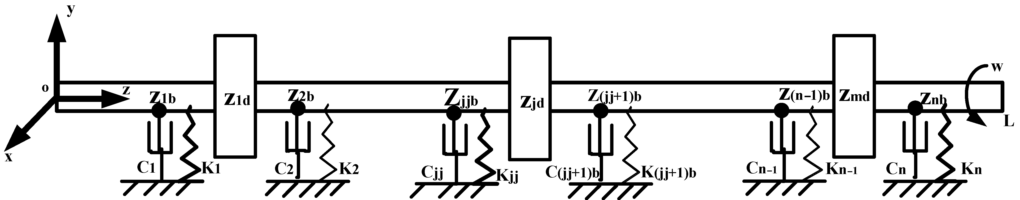
2.1. Revisting the CRDAM
2.2. Single Direction Algorithm
2.3. Two Orthogonal Direction Algorithms
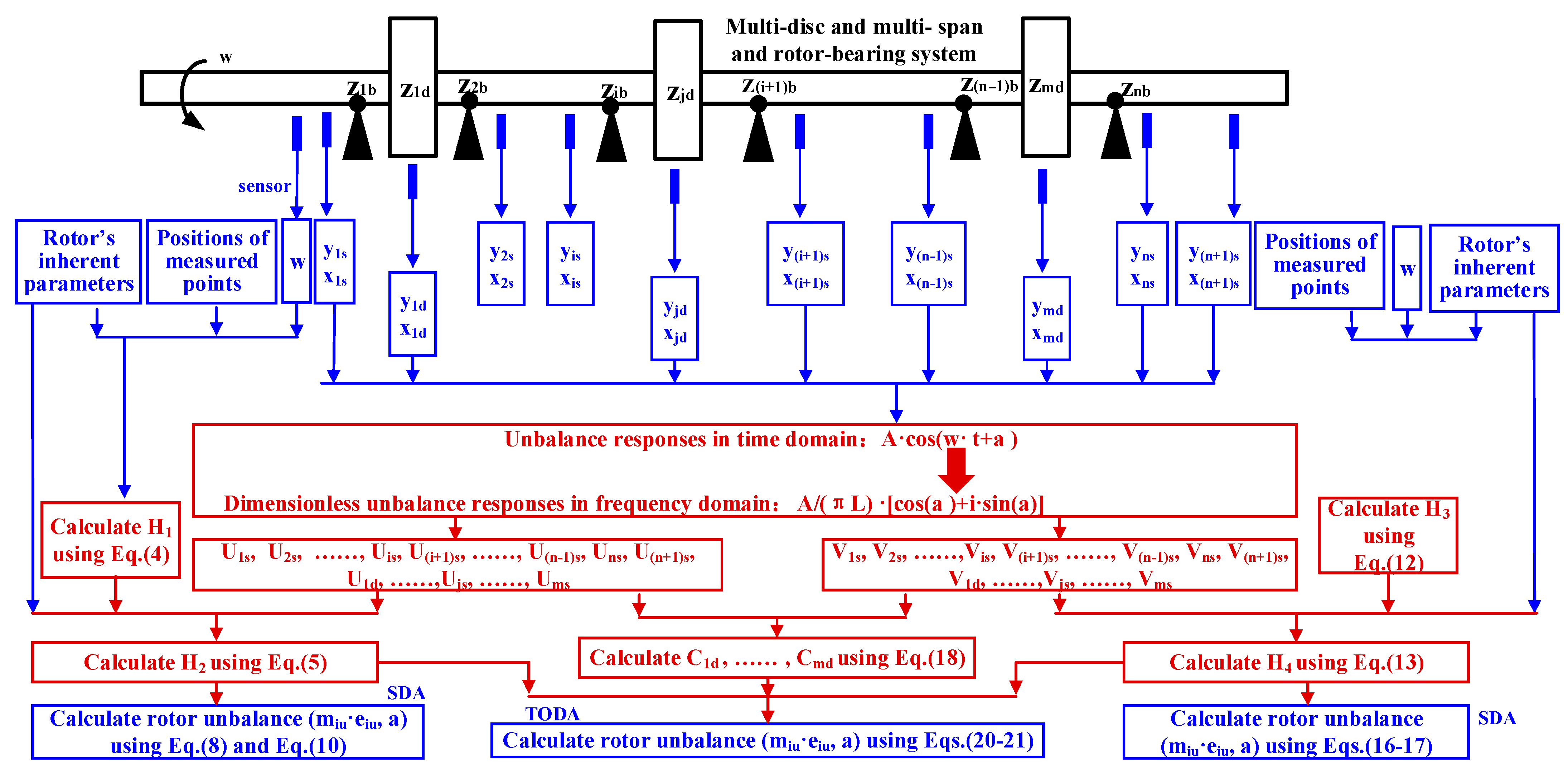
2.4. Identification Procedures of the Two Algorithms
3. Numerical Simulations and Discussion
3.1. Methodology of the Numerical Simulations
3.2. Accuracy of SDA and TODA
3.2.1. Results
- (1)
- Results of the first kind of simulation
- (2)
- Results of the second kind of simulation
3.2.2. Discussion
3.3. Adjustment Point
3.3.1. Results
- (1)
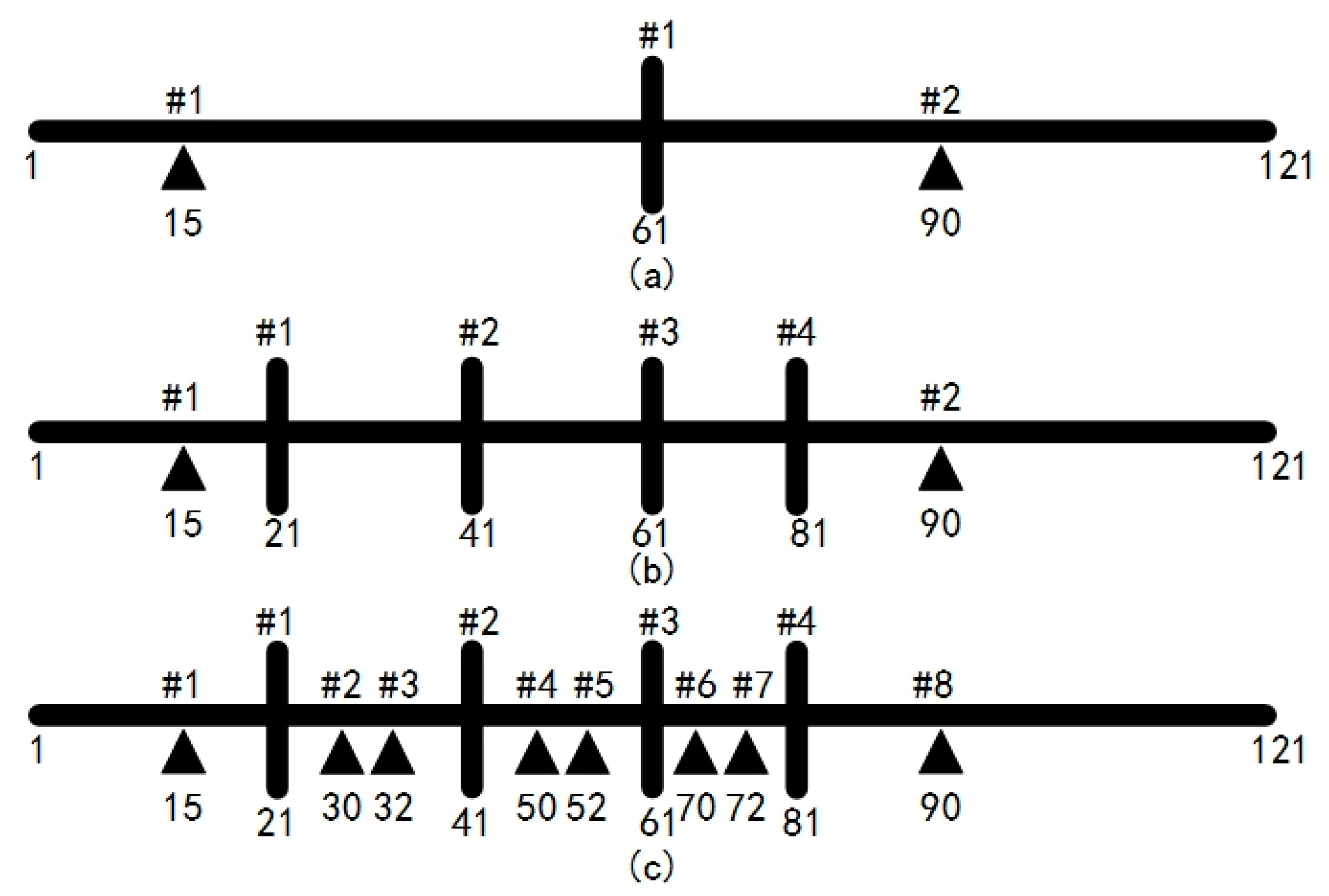
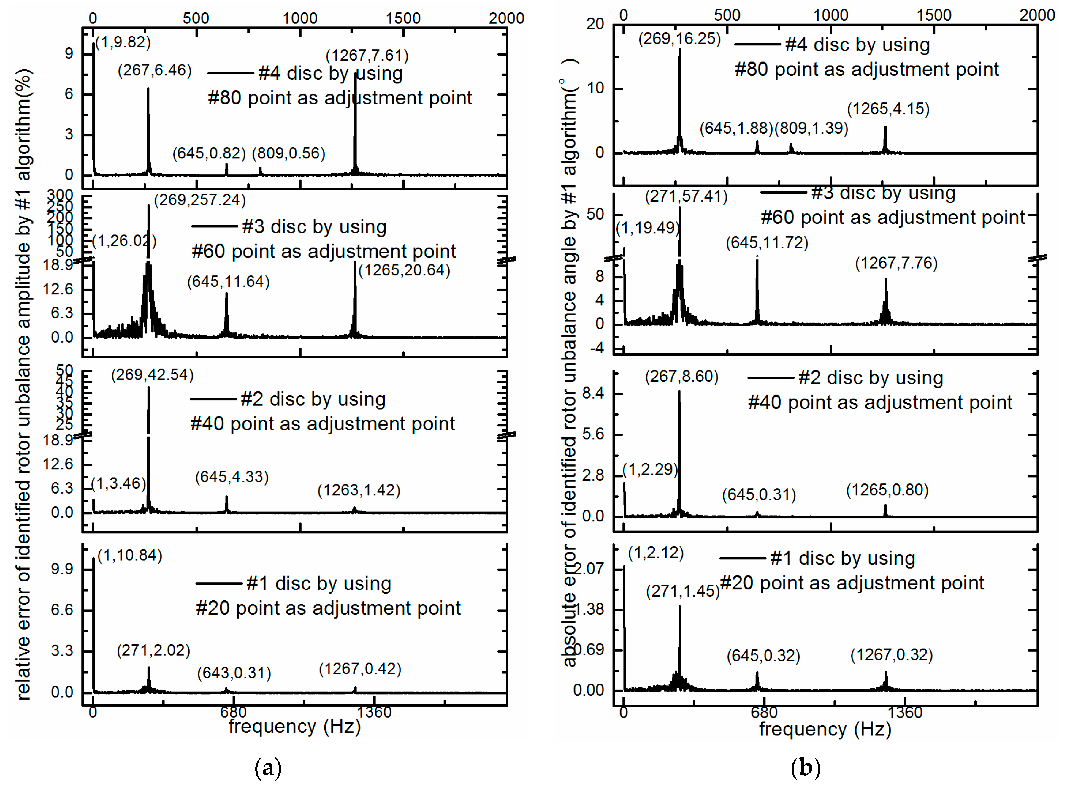
- According to Equations (24) and (25), for SDA, when #20 point, which is near #1 disc, is used as one of the required measuring points, the maximum identification error for rotor unbalance for #1 disc is the smallest among that of the four discs. The maximum identification error for rotor unbalance is 10.84%∠2.12°, while for #2–4 discs, their maximum errors are much bigger. When #40 point, which is close to #2 disc is used, the maximum identification error for rotor unbalance for #2 disc becomes the smallest. It is 42.54%∠8.60°. When #60 point, which is beside #3 disc, is used, #3 disc’s rotor unbalance identification error, which is 257.24%∠57.41°, is the second smallest and is close to the smallest error of 254.72%∠51.14°. When #80 point, which is beside #4 disc, is used, #4 disc’s rotor unbalance identification error, which is 9.82%∠16.25°, is much smaller than the others. From the perspective of the column in the matrix, when the measuring point is changed from #20 to #40, the maximum identification error for rotor unbalance for #1 disc becomes bigger, while the maximum identification error for rotor unbalance for #4 disc becomes smaller. The maximum identification errors for rotor unbalance for #2 and #3 discs are also changed apparently. As #20 point is applied, #1 disc acquires the best recognition accuracy, while #2 disc has the best recognition accuracy as #40 point is applied, #3 disc has the best recognition accuracy as #60 point is applied, and #4 disc has the best recognition accuracy as #80 point is applied.
- (2)
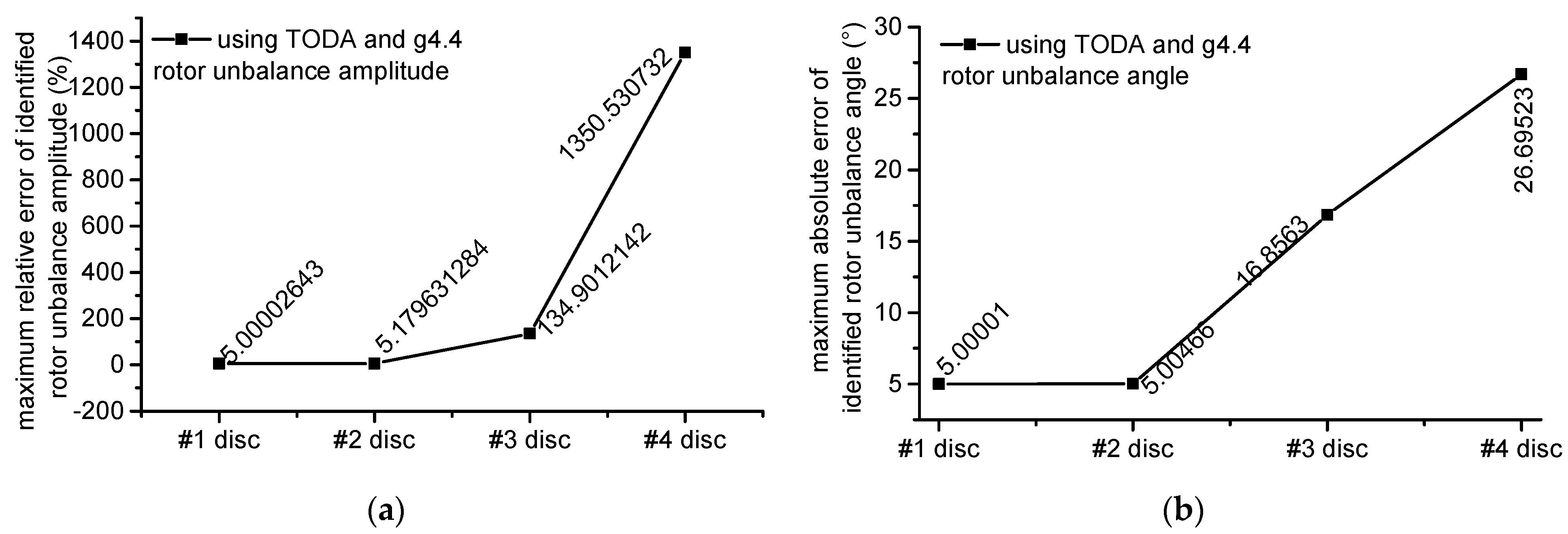
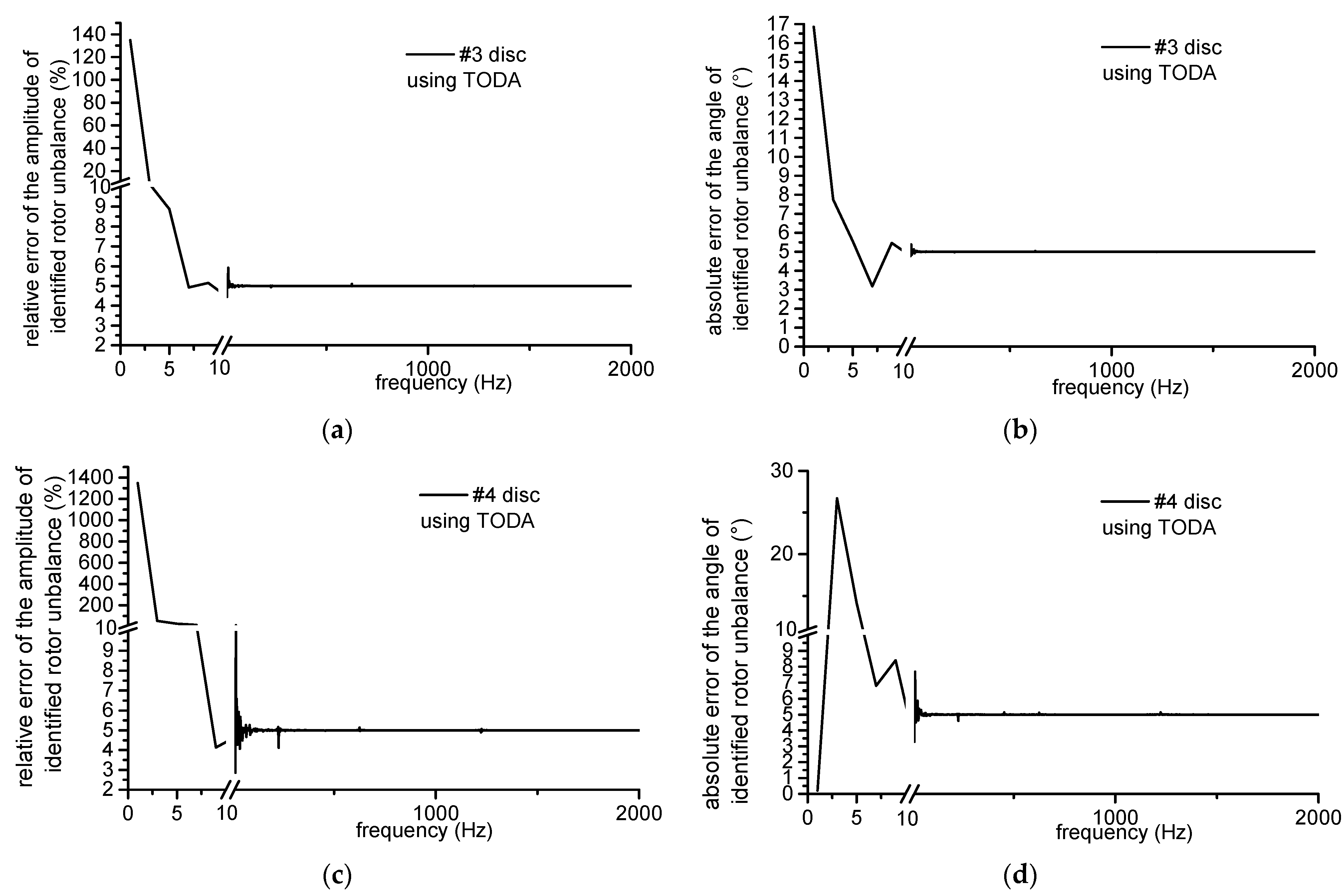
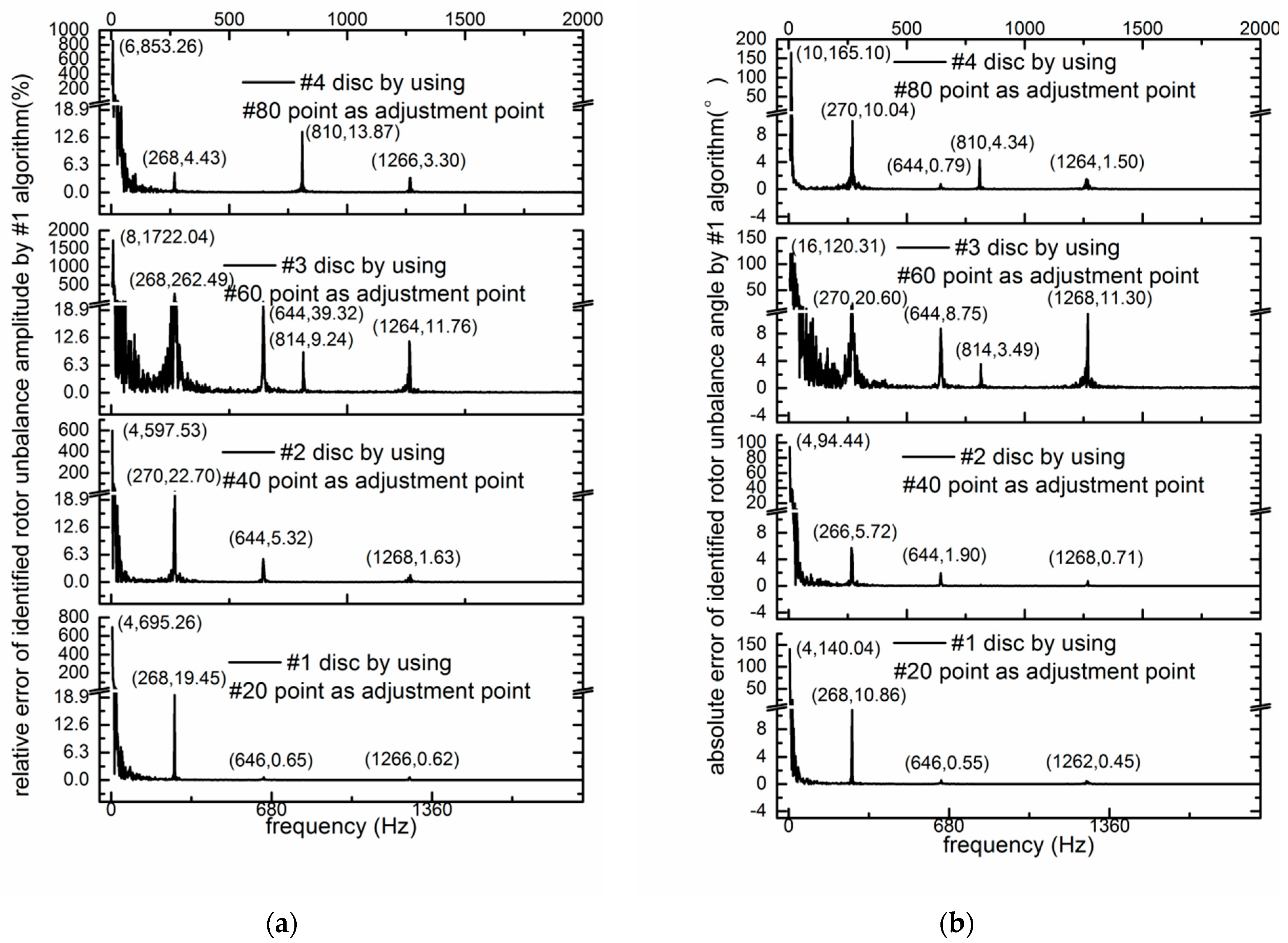
- As for TODA, similar results can be obtained, although the values of maximum identification errors are much bigger than the maximum identification errors for SDA, according to Equations (26) and (27). When #20 point, which is near #1 disc, is used as one of the required measuring points, the maximum identification error for rotor unbalance for #1 disc is the smallest among that of the four discs. The maximum identification error for rotor unbalance is 4.22 × 10²%∠170.38°, while for #2–4 disc, their maximum errors are much bigger. When #40 point, which is close to #2 disc, is used, the maximum identification error for rotor unbalance for #2 disc becomes the smallest. It is 1.64 × 10⁴%∠140.73°. When #60 point, which is beside #3 disc, is used, #3 disc’s rotor unbalance identification error, which is 6.03 × 10⁴%∠179.57°, is the second smallest. When #80 point, which is beside #4 disc, is used, #4 disc’s rotor unbalance identification error is 2.68 × 10¹⁵%∠179.95°. Although it is the biggest among the obtained maximum identification errors of the four discs, it is the smallest error for #4 disc, which can be obtained by changing the measuring point from #20 to #40. From the perspective of the column in the matrix, when the measuring point is changed from #20 to #40, the maximum identification error for rotor unbalance for #1 disc becomes bigger. The maximum identification errors of rotor unbalance for #2, #3, and #4 discs are also changed apparently. As #20 point is applied, #1 disc acquires the best recognition accuracy, while #2 disc has the best recognition accuracy as #40 point is applied, #3 disc has the best recognition accuracy of unbalance amplitude as #60 point is applied, and #4 disc has the best recognition accuracy as #80 point is applied.
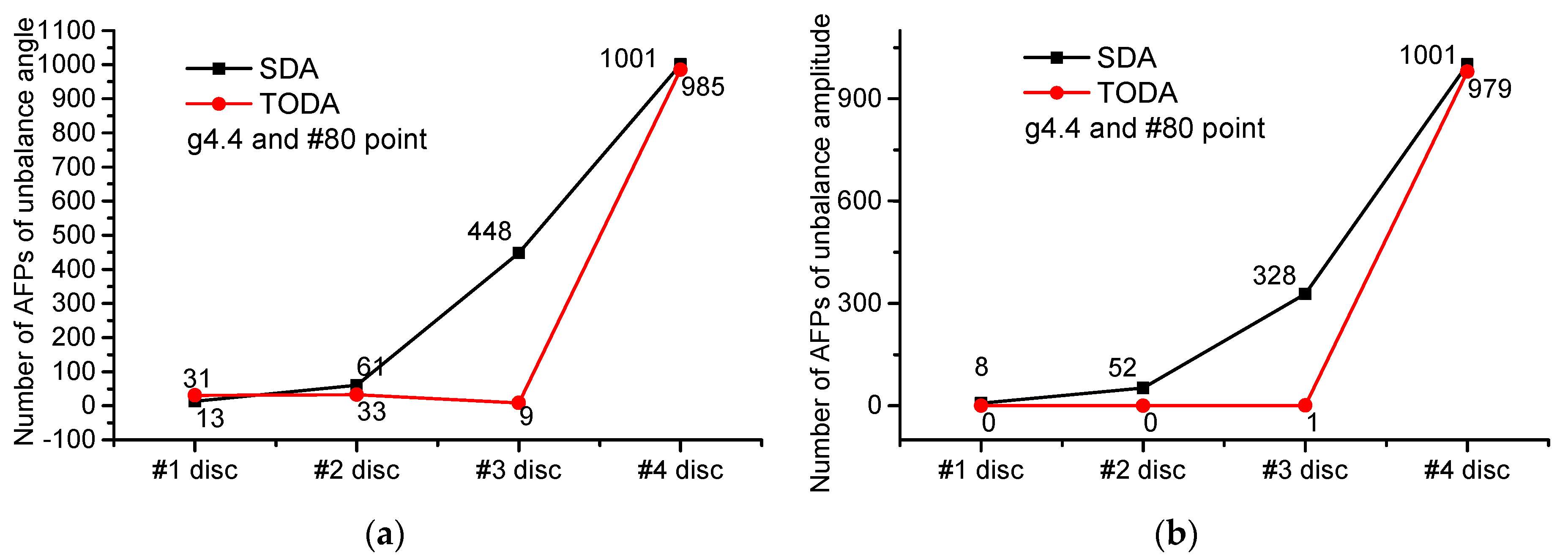
- (1)
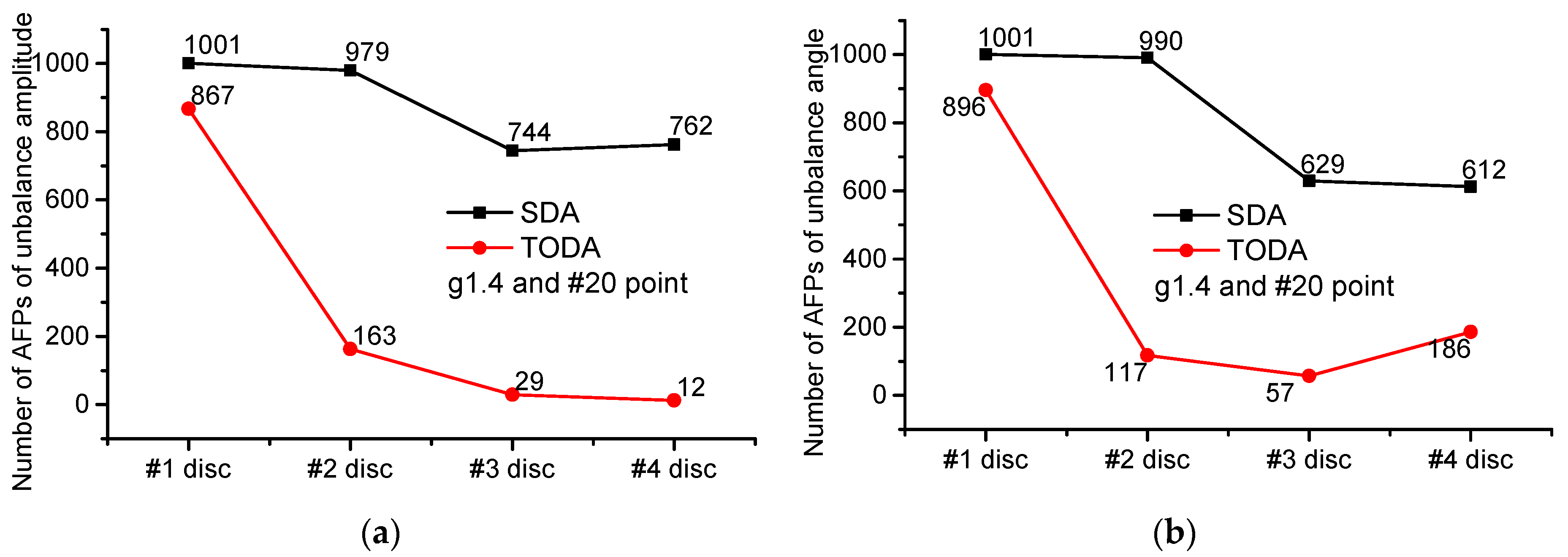
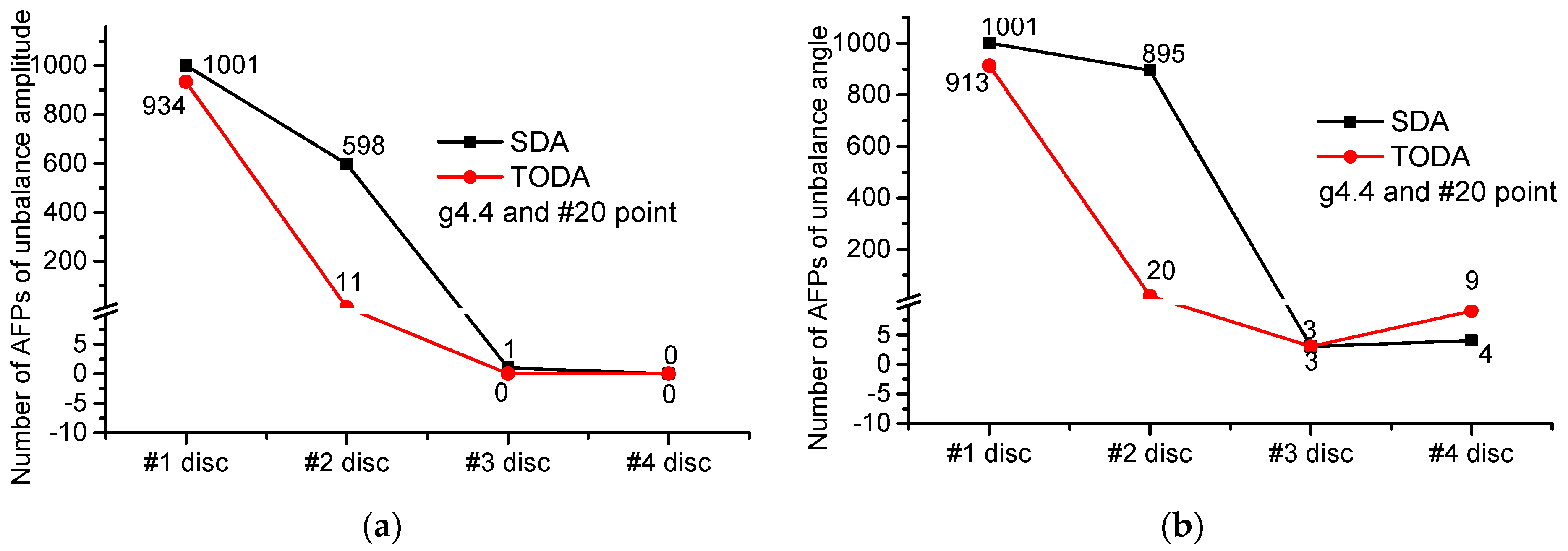
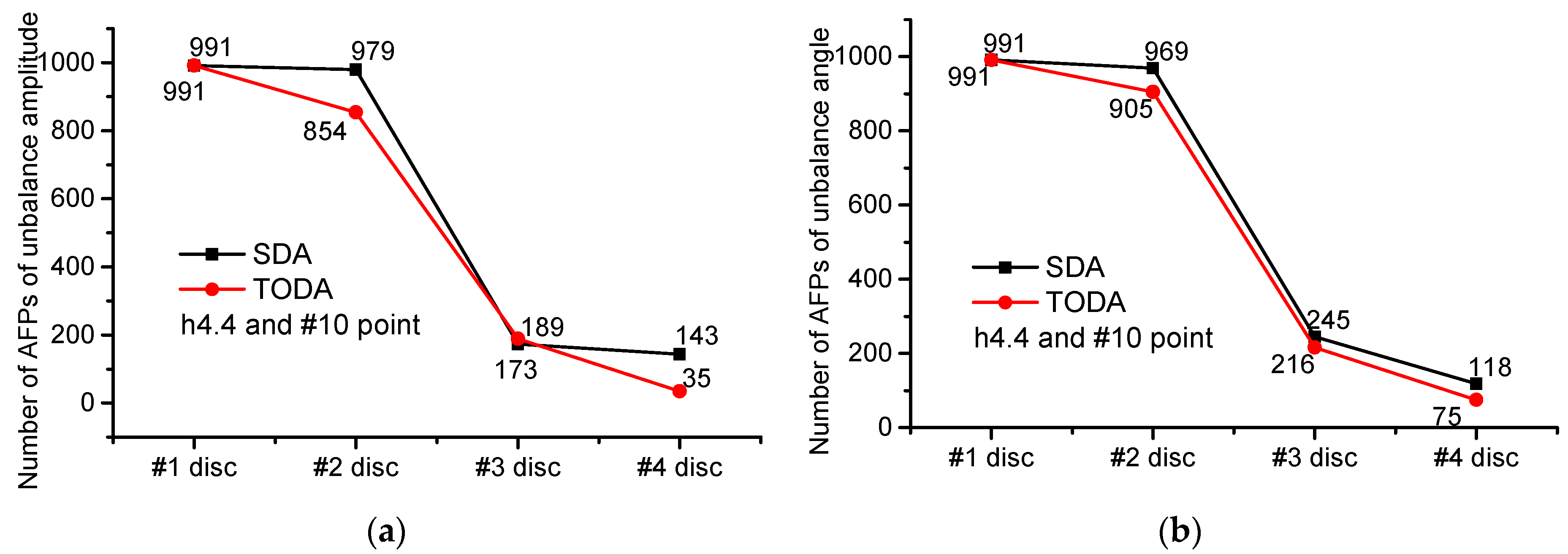
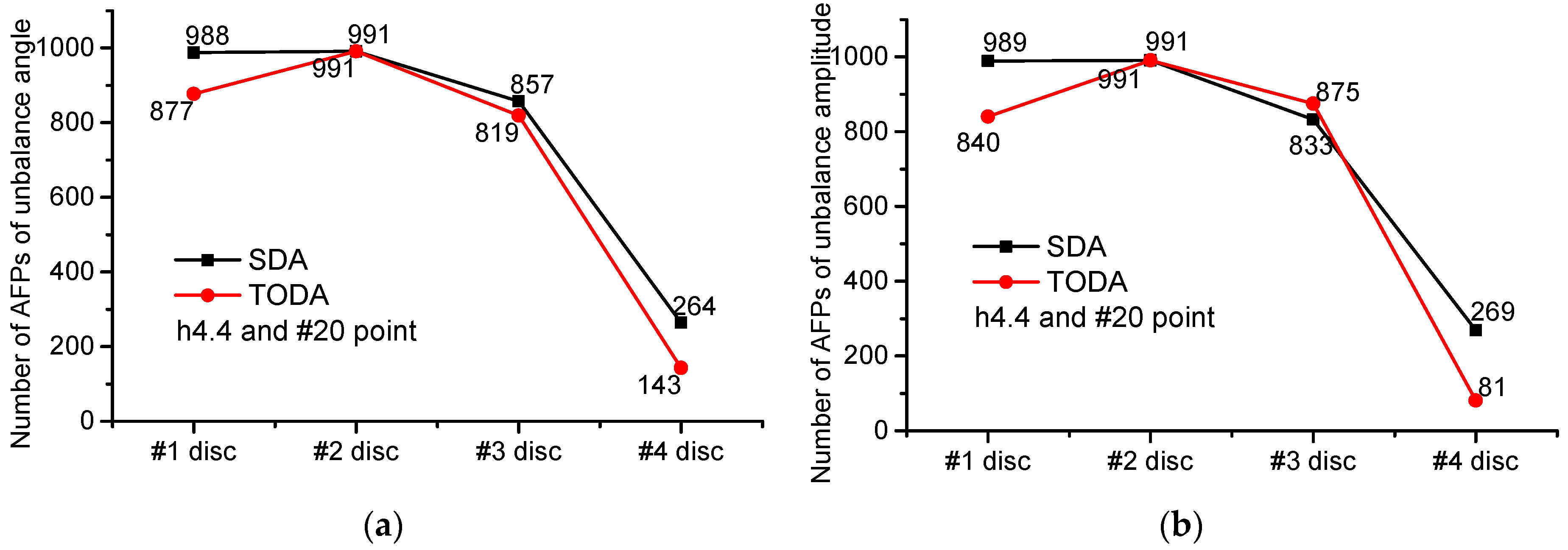
- The numbers of AFPs of rotor unbalance amplitude for #1–#4 discs are 1001, 979, 744, and 762, respectively, according to Figure 15a. For the rotor unbalance angle, there are 1001, 990, 629, and 612 AFPs, respectively, according to Figure 15b. This indicates that the identification results for rotor unbalance for #1 disc are best when #20 point is used as one of the required measuring points.
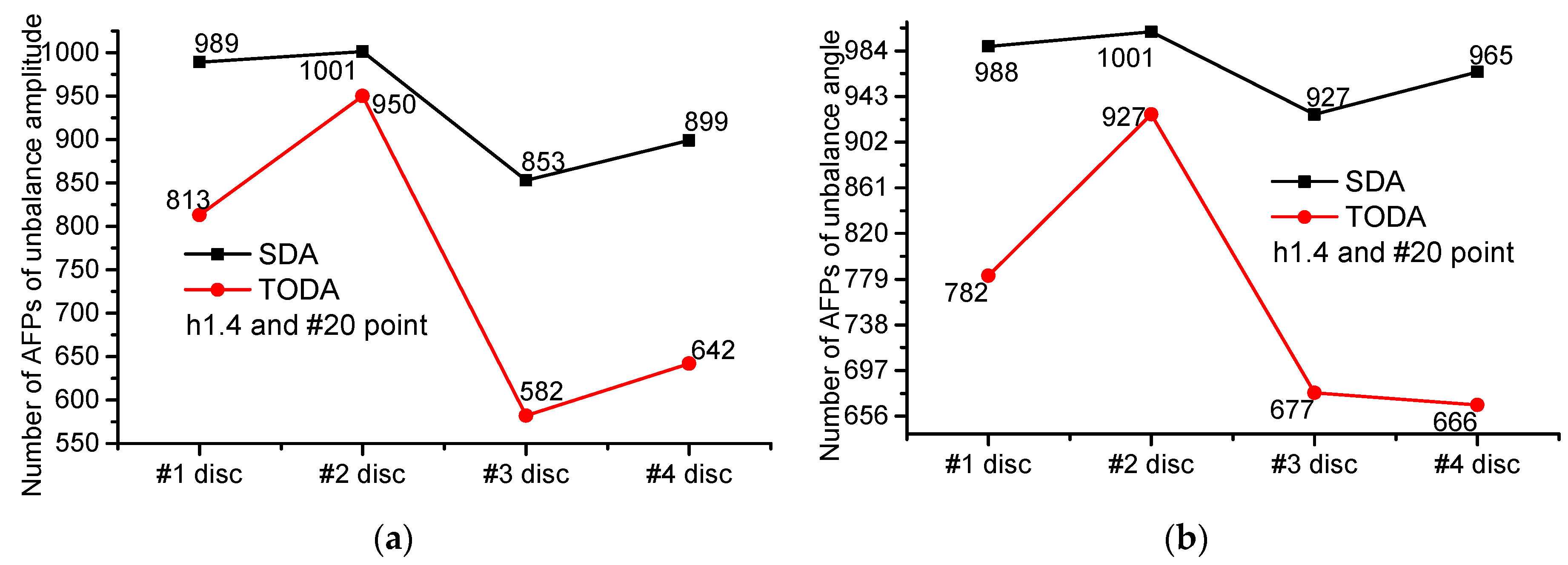
- (2)
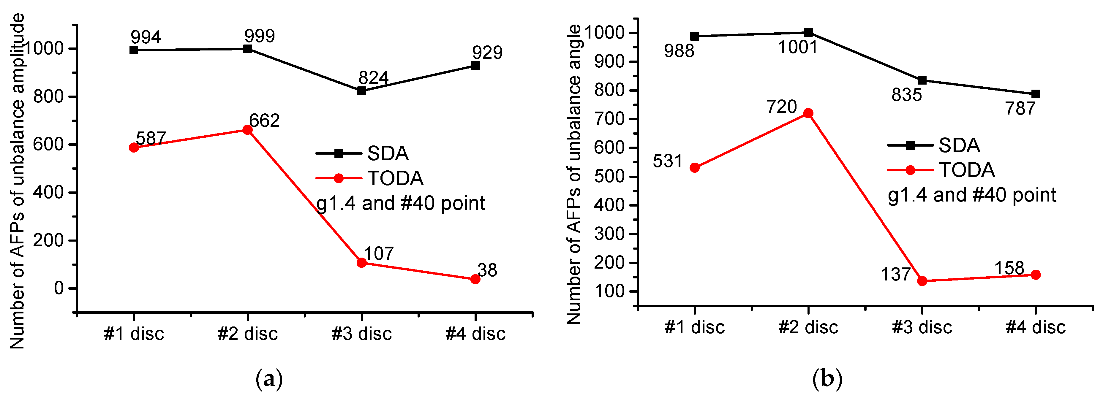
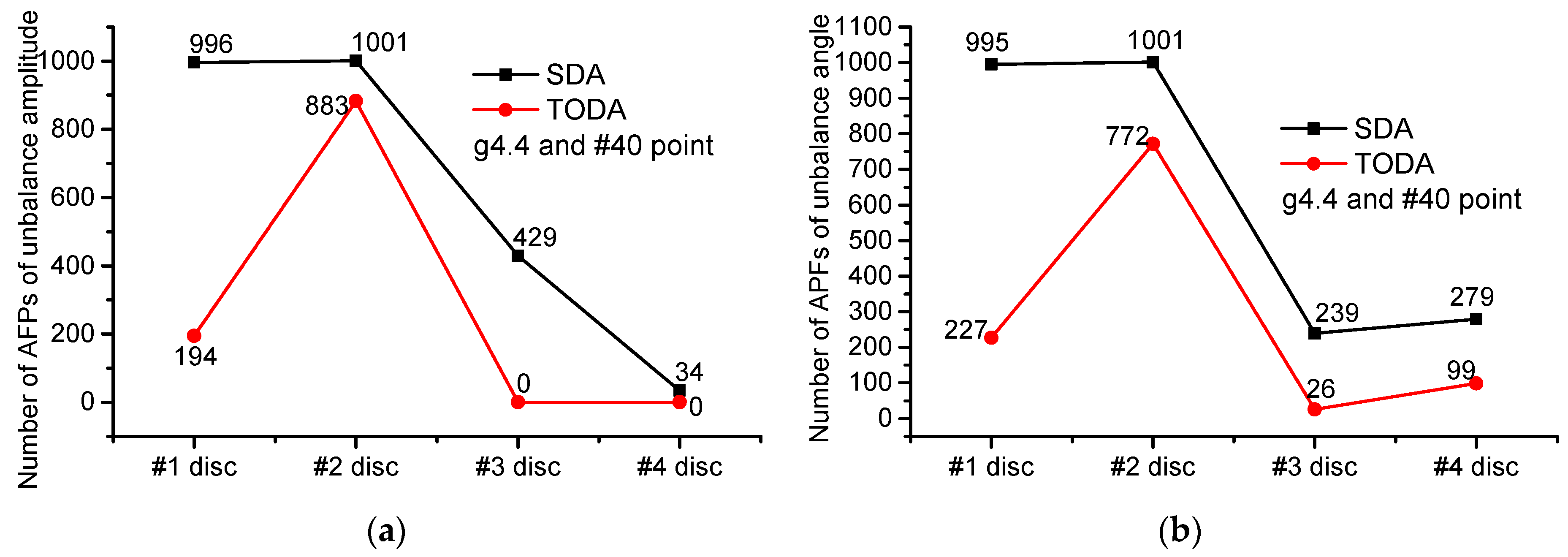
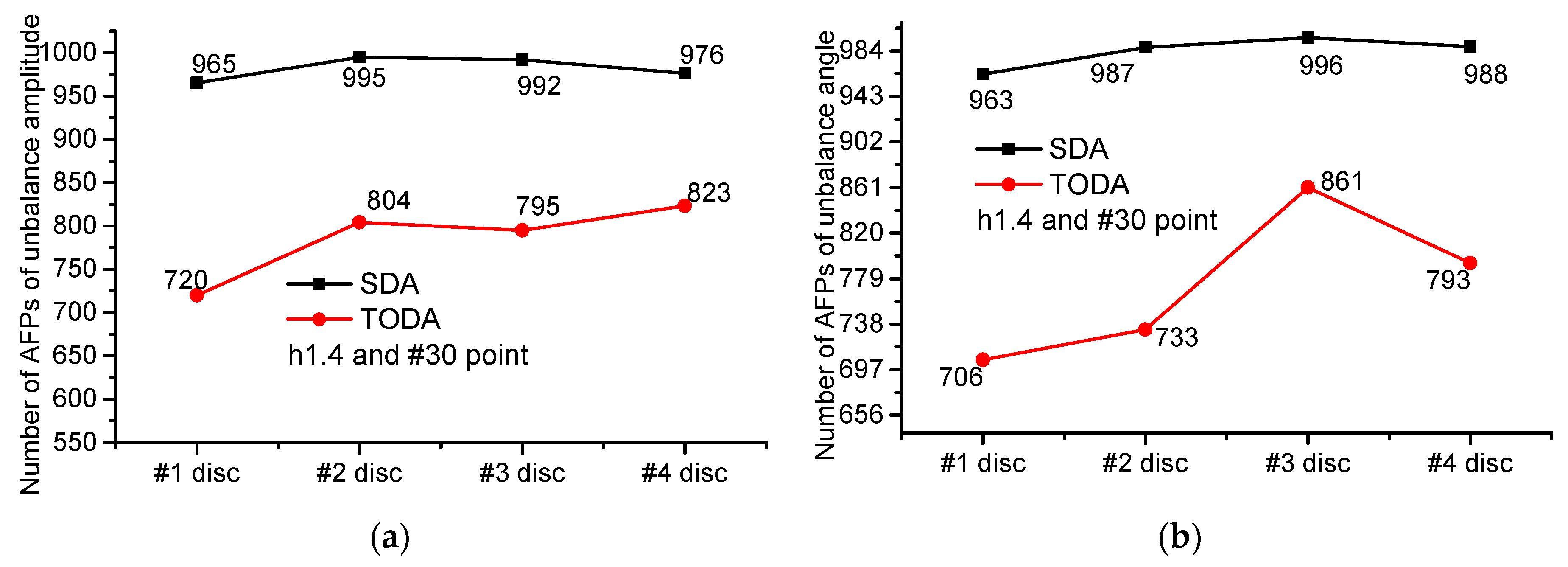
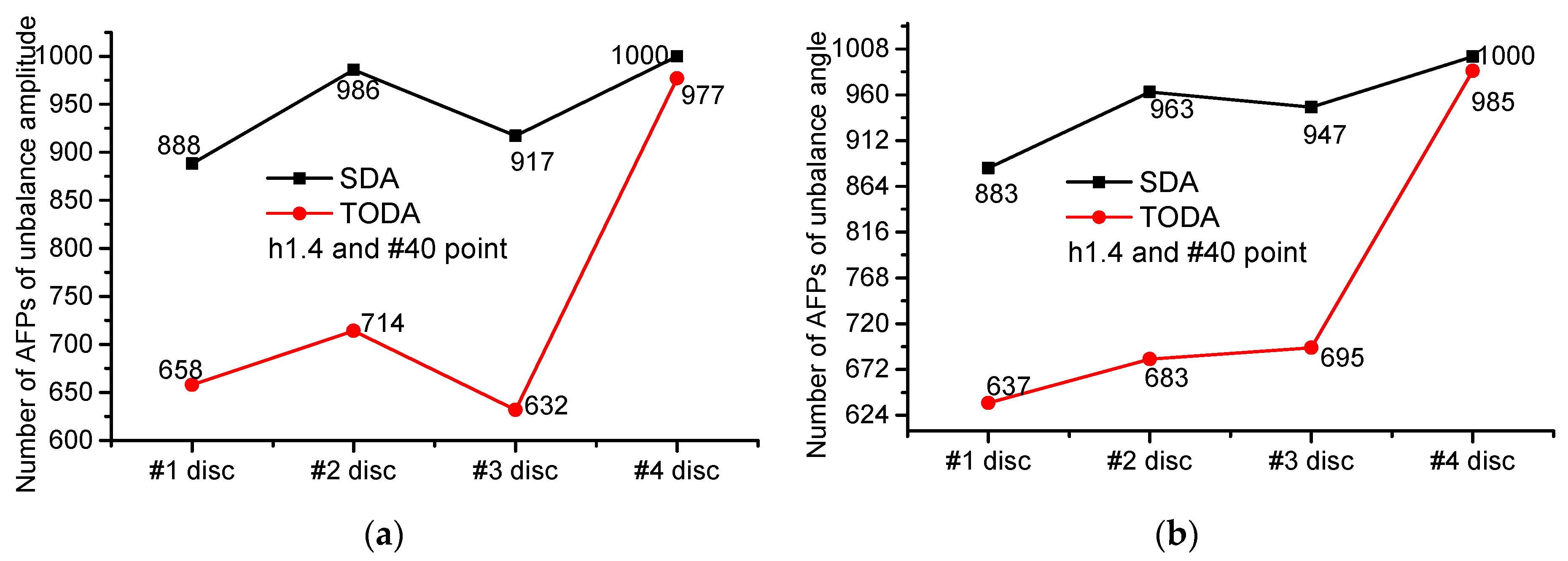
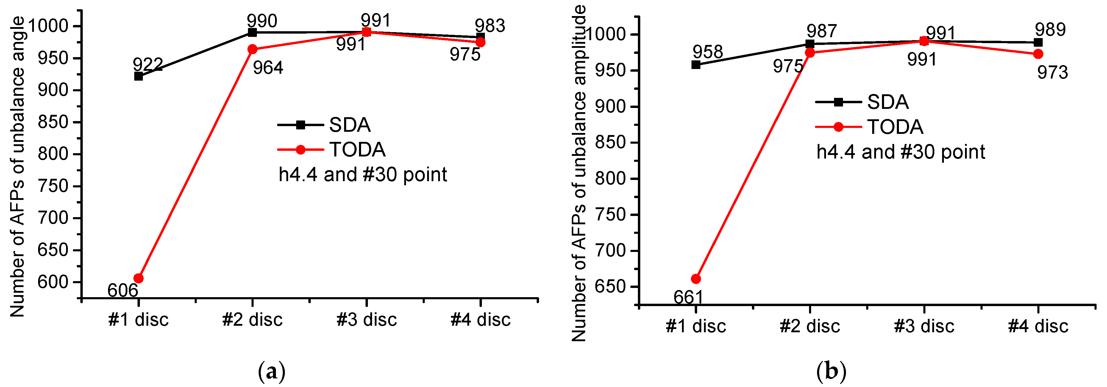
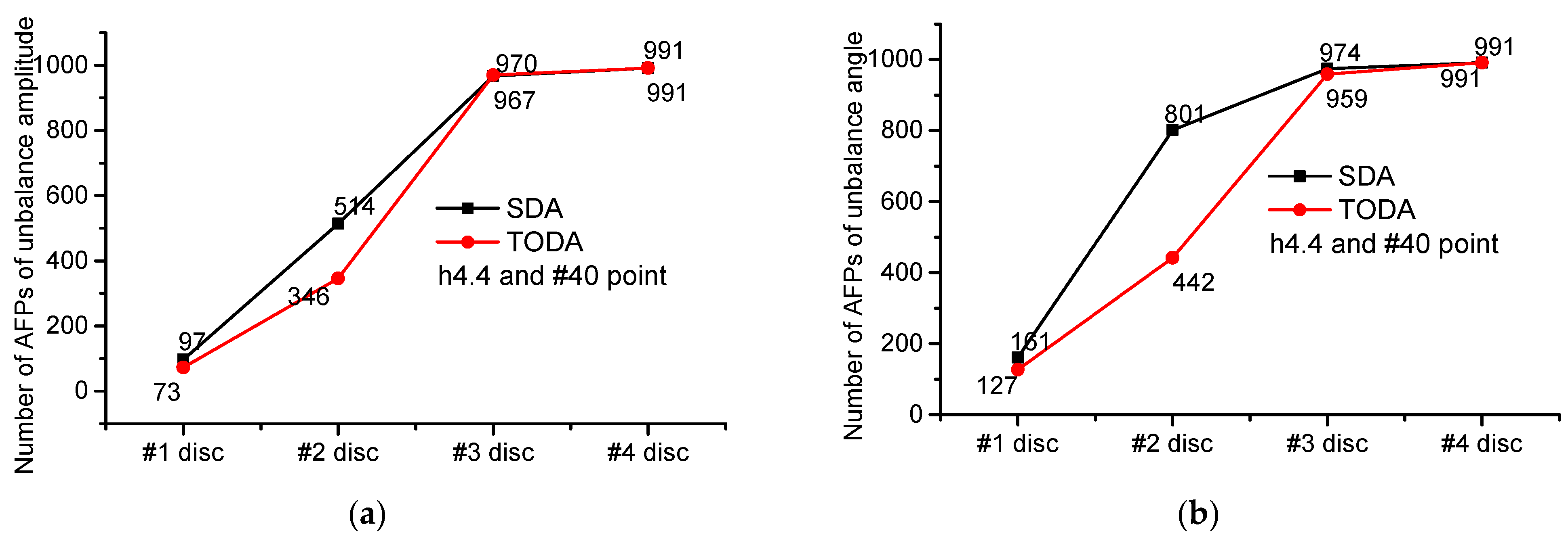
- According to Figure 16, there are 994, 999, 824, and 929 AFPs, respectively, for the rotor unbalance amplitude of #1 disc, #2 disc, #3 disc, and #4 disc, and 988, 1001, 835, and 787 AFPs, respectively, for the rotor unbalance angle. This indicates that the identification results for rotor unbalance for #2 disc are best when #40 point is used as one of the required measuring points.
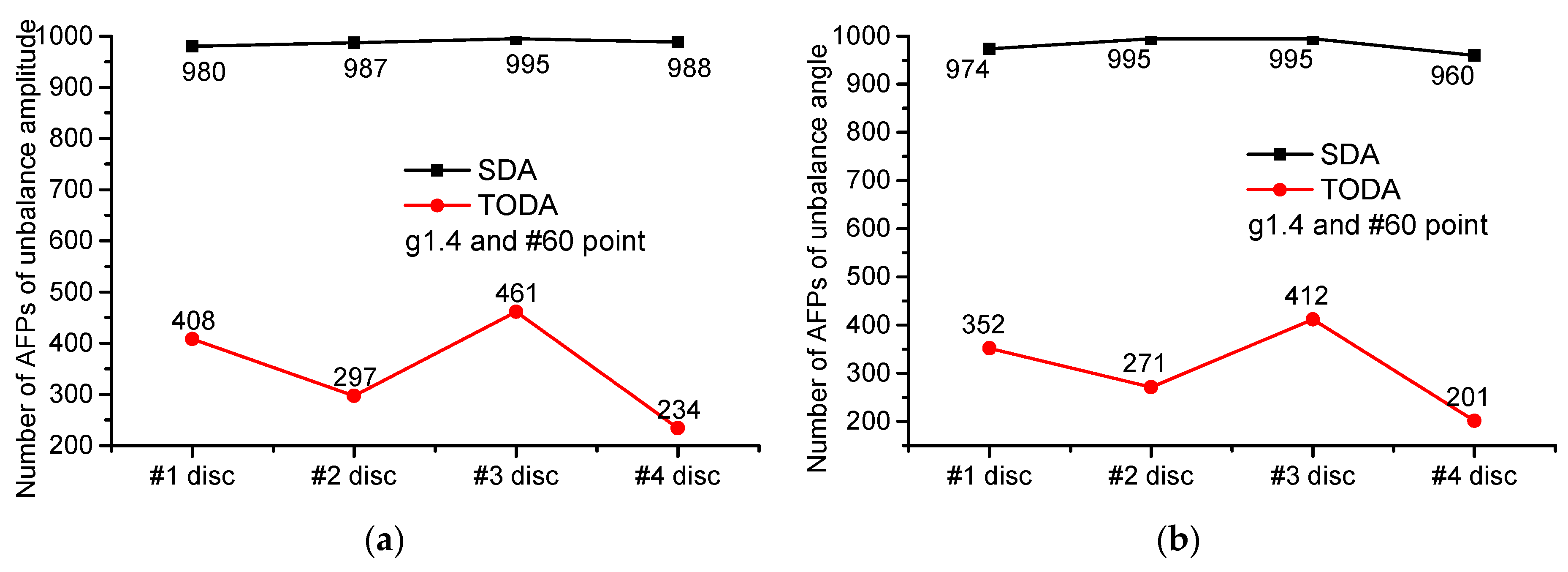
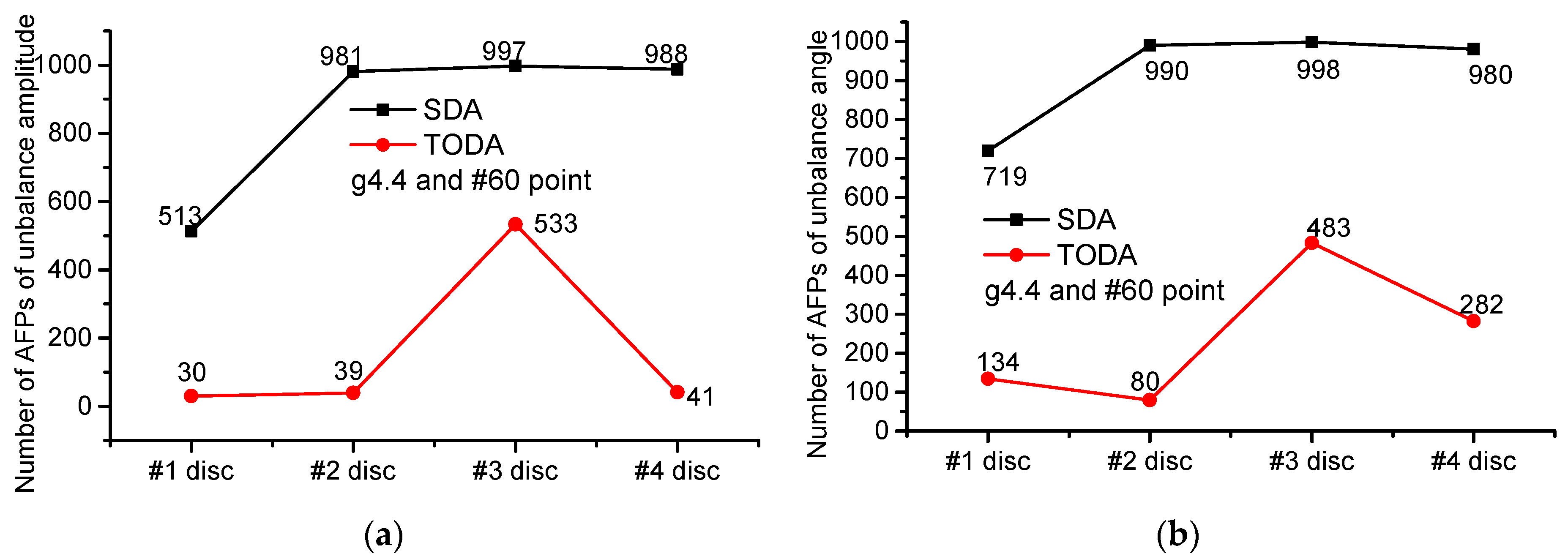
- (3)
- According to Figure 17, the numbers of AFPs of rotor unbalance amplitude are 980, 987, 995, and 988, respectively, and the numbers of rotor unbalance angles are 974, 995, 995, and 960 respectively. This indicates that the identification results for rotor unbalance for #3 disc are best when #60 point is used as one of the required measuring points.
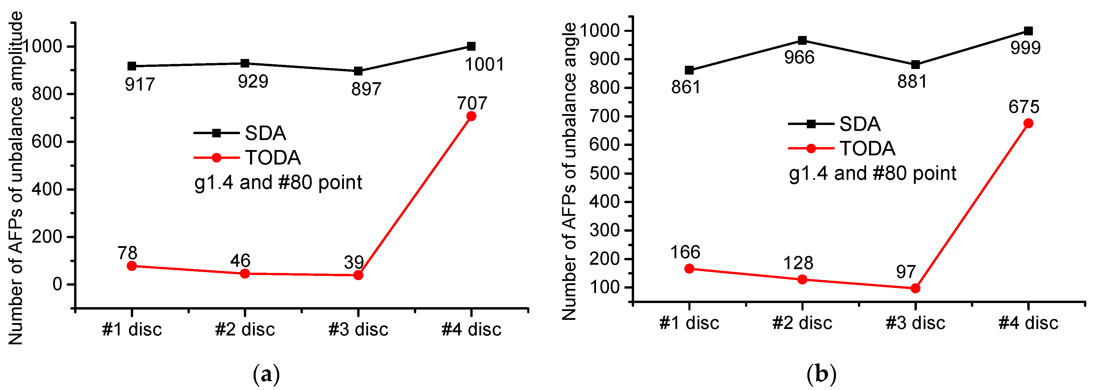
- (4)
- According to Figure 18, for the rotor unbalance amplitude of #1 disc, #2 disc, #3 disc, and #4 disc, there are 917, 929, 897, and 1001 AFPs, respectively. For the angle, there are 861, 966, 881, and 999 AFPs, respectively. This indicates that the identification results for rotor unbalance for #4 disc are best when #80 point is used as one of the required measuring points.
3.3.2. Discussion
3.4. Affect of Sensor Resolution
3.4.1. Results
- (1)
- Sensor resolution of 0.1 nm
- (2)
- Sensor resolution of 1 nm
- (3)
- Sensor resolution of 0.1 um
- (4)
- Sensor resolution of 1 um
- (5)
- According to the above results, the peak values that were outside the assumed allowable range—the amplitudes bigger than 20% and the angles bigger than 10°—are all counted in Table 7, Table 8, Table 9 and Table 10, with the sensor resolutions set at 0.1 nm, 1 nm, 0.1 um, and 1 um, respectively. From Table 7, Table 8, Table 9 and Table 10, the frequencies at which these peak values appear are at or around the critical frequencies listed in Table 11 and the low frequencies such as 1 Hz, 4 Hz, and so on. This indicates that the rotor unbalance identification error is big when the rotor works at a low speed or near the critical speeds when using SDA.
3.4.2. Discussion
- (1)
- At a low frequency, the peak values of identification errors become bigger as sensor resolution is reduced and rotor unbalance cannot be identified when the sensor resolution is 1 um.
- (2)
- At or around the first order critical frequency, the identification error, which is obtained using a sensor resolution of 0.1 nm, is little different from the identification error obtained using a sensor resolution of 1 nm. The identification error becomes much bigger when the sensor resolution is 0.1 um and the rotor unbalance cannot be identified when the sensor resolution is close to 1 um.
- (3)
- At or around the second order critical frequency, the identification error obtained when the sensor resolution is 0.1 nm is equal to the identification error obtained when the sensor resolution is 1 nm. However, when the sensor resolution is 0.1 um, the identification error becomes a little bigger. Moreover, when the sensor resolution comes close to 1 um, the rotor unbalance cannot be identified.
- (4)
- At or around the third order critical frequency, the identification error obtained when the sensor resolution is 0.1 nm is equal to the identification error obtained when the sensor resolution is 1 nm. However, when the sensor resolution comes close to 0.1 um and 1 um, the identification errors become a little bigger.
4. Conclusions
- (1)
- The proposed algorithms provide a technique with which to monitor all the rotor unbalances on-line under operational conditions. For SDA, the unbalance responses in only one direction are needed. For a rotor with discs and bearings, the number of required unbalance responses is m + n + 1. While for TODA, the unbalance responses in both the and directions are required. The necessary measuring position of the two methods should be at the disc whose unbalance is to be monitored. For monitoring the unbalance of all discs, there should be a sensor mounted at each disc, while the other measuring positions can be at or around the bearings or discs. Moreover, numerical simulations indicate that there should be one measuring point called the adjustment point to achieve a high identification accuracy. The proposed adjustment point should be near the disc whose unbalance is to be monitored. In order to identify all the discs’ unbalances accurately and simultaneously, there should be measuring points, among which adjustment points near each disc are necessary.
- (2)
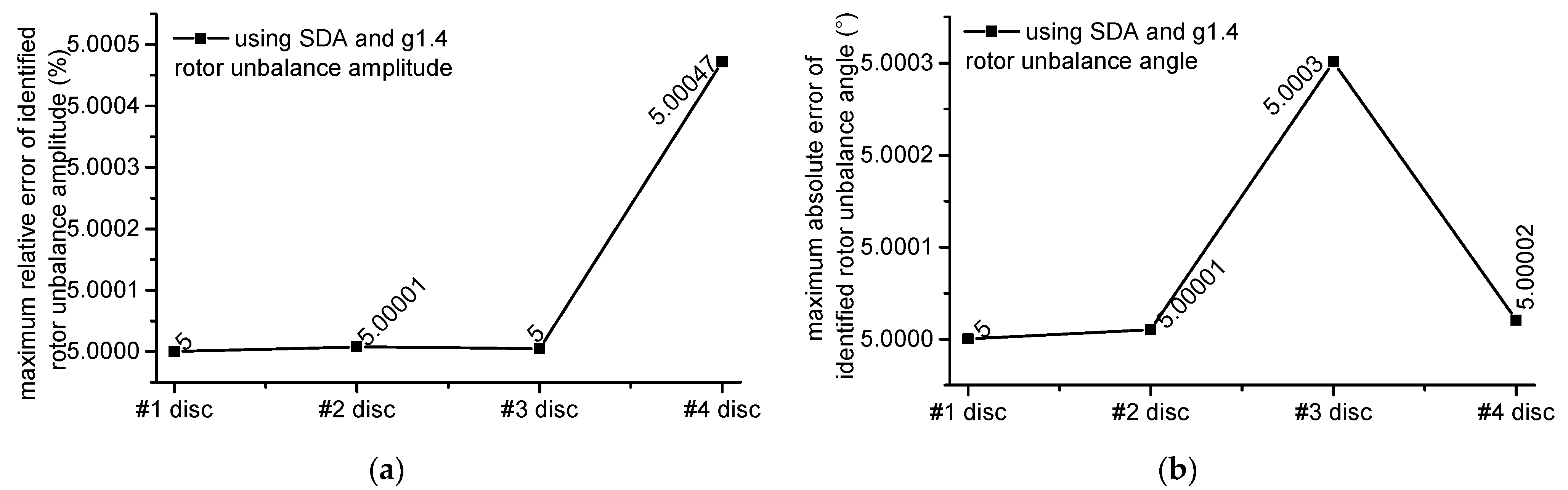
- The identification accuracy of the proposed algorithms requires a high performance of the unbalance response measurement system. Numerical simulations indicate that if the measuring errors of all the required unbalance responses are zero, the identification error will be zero, too. When the measuring errors are the same, the identification error will be equal to the measuring errors. It is indicated that the consistency of each channel’s measurement errors plays a critical role in identifying rotor unbalance when using the proposed algorithms. In addition, SDA has a better identification accuracy than TODA when considering sensor resolution from the perspective of engineering applications. The identification error of SDA is only high at a very low frequency and the critical frequencies when sensor resolutions are considered. Hence, SDA is suitable for medium-speed and high-speed rotors. Moreover, identification accuracy is strongly related to sensor resolution. Sensors with resolutions of 1 um should be avoided and sensors with 1 nm and 0.1 nm resolutions are recommended.
Author Contributions
Funding
Institutional Review Board Statement
Informed Consent Statement
Data Availability Statement
Conflicts of Interest
Nomenclature
| Dimensionless value of position due on the z-axis | ||
| Dimensionless unbalance response in the frequency domain due on the y-axis | ||
| Dimensionless unbalance response in the frequency domain due on the x-axis | ||
| For instance, #1 disc means the first disc | ||
| Eccentric masses of disc | ||
| Eccentric distance of disc | ||
| Eccentric angle of disc | ||
| Masses of disc | ||
| Rotation frequency rotors | ||
| Length of rotor shaft | ||
| Elastic modulus of rotor shaft | ||
| Diametric shaft cross-sectional geometric moment of inertia | ||
| bearing’s main stiffness coefficient in the direction | ||
| bearing’s cross-coupled stiffness coefficient in the direction | ||
| bearing’s cross-coupled stiffness coefficient in the direction | ||
| bearing’s main stiffness coefficient in the direction | ||
| bearing’s main damping coefficient in the direction | ||
| bearing’s cross-coupled damping coefficient in the direction | ||
| bearing’s cross-coupled damping coefficient in the direction | ||
| bearing’s main damping coefficient in the direction | ||
| Bearing’s main complex coefficient in the direction | ||
| Bearing’s cross-coupled complex coefficient in the direction | ||
| Bearing’s cross-coupled complex coefficient in the direction | ||
| Bearing’s main complex coefficient in the direction | ||
| coordinate position of # disc | ||
| coordinate position of # bearing | ||
| Dimensionless value of | ||
| Dimensionless value of | ||
| Green’s functions in the direction | ||
| Green’s functions in the direction | ||
| Green’s coefficients for # disc in the direction | ||
| Green’s coefficients for # bearing in the direction | ||
| Green’s coefficients for # disc in the direction | ||
| Green’s coefficients for # bearing in the direction | ||
| disc’s dimensionless unbalance response in frequency domain in the direction | ||
| disc’s dimensionless unbalance response in frequency domain in the direction | ||
| bearing’s dimensionless unbalance response in frequency domain in the direction | ||
| bearing’s dimensionless unbalance response in frequency domain in the direction | ||
| Number of discs | ||
| Number of bearings | ||
Appendix A
- (1)
- Simulation results for g1.1 and h1.1

| Methods | Rotor Unbalance | g1.1 | h1.1 |
|---|---|---|---|
| SDA | Amplitude | 6.77977 × 10⁻⁹ | 1.23934 × 10⁻⁸ |
| Angle | 1.6455 × 10⁻⁹ | 7.73824 × 10⁻⁹ | |
| TODA | Amplitude | 4.21247 × 10⁻⁵ | 2.79355 × 10⁻⁸ |
| Angle | 3.32871 × 10⁻⁶ | 2.49249 × 10⁻⁸ |
- (2)
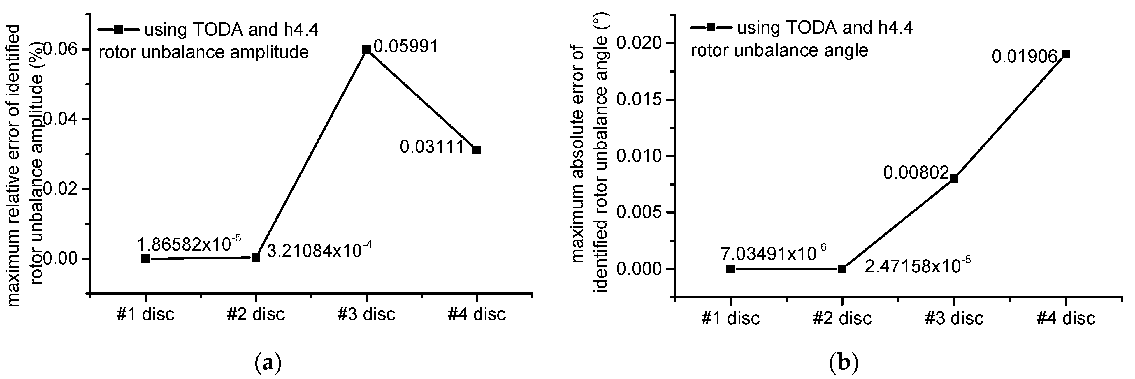
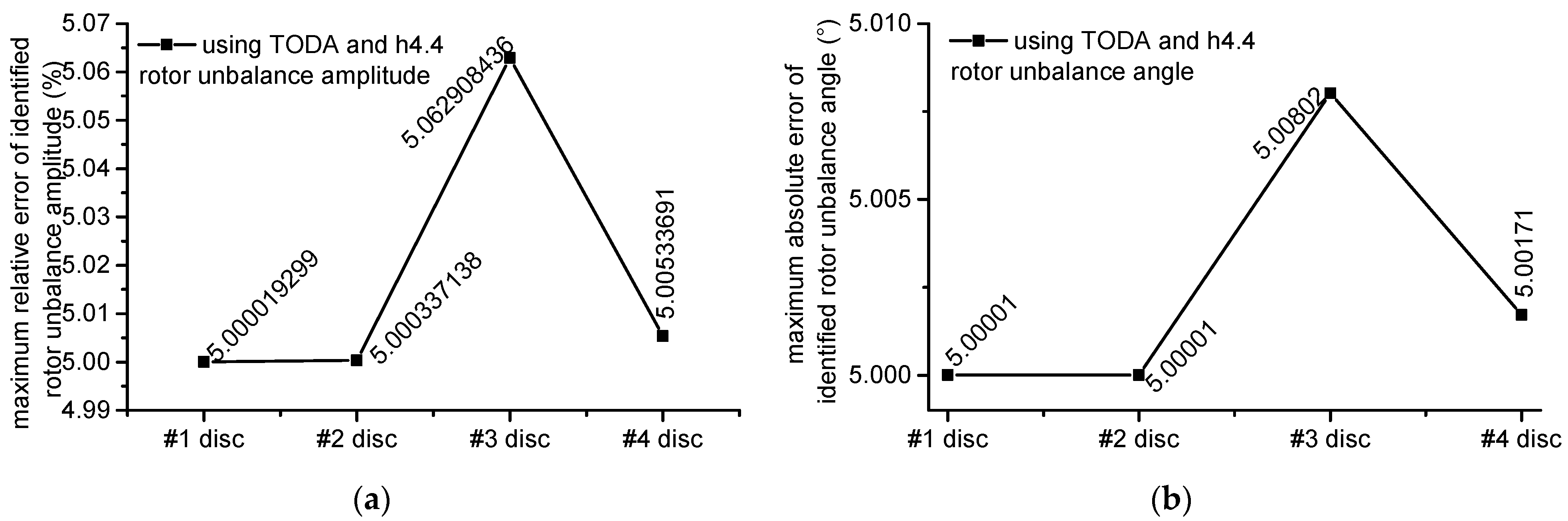
- Simulation results for rotor h4.4


- (3)
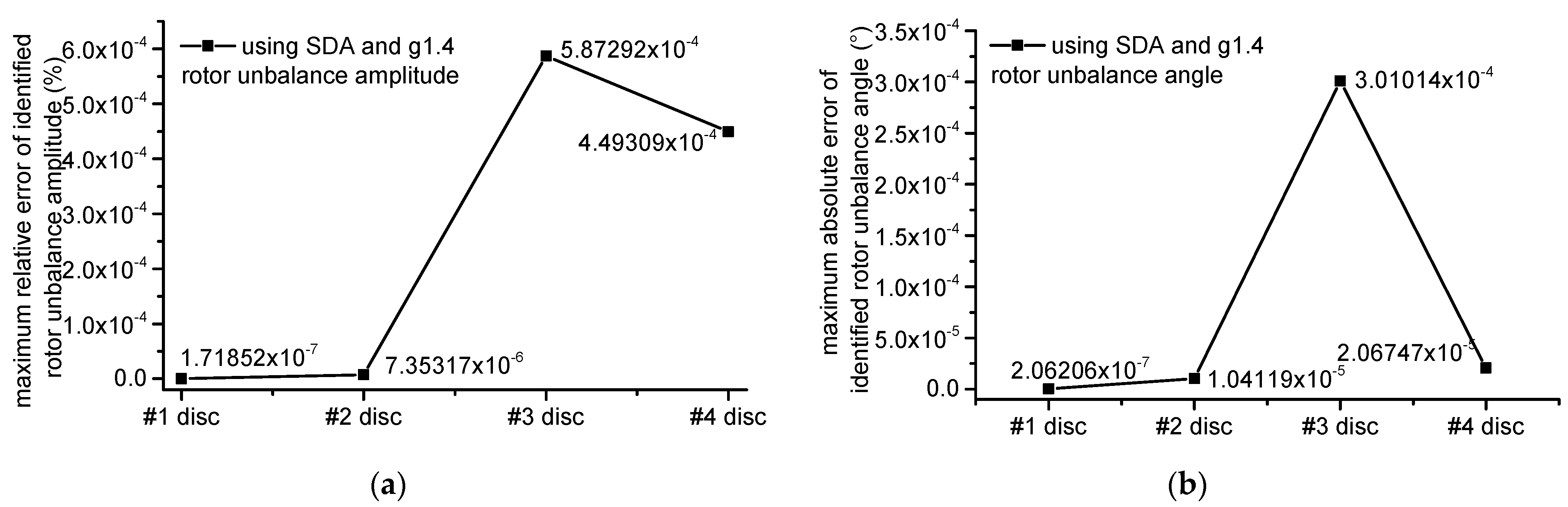
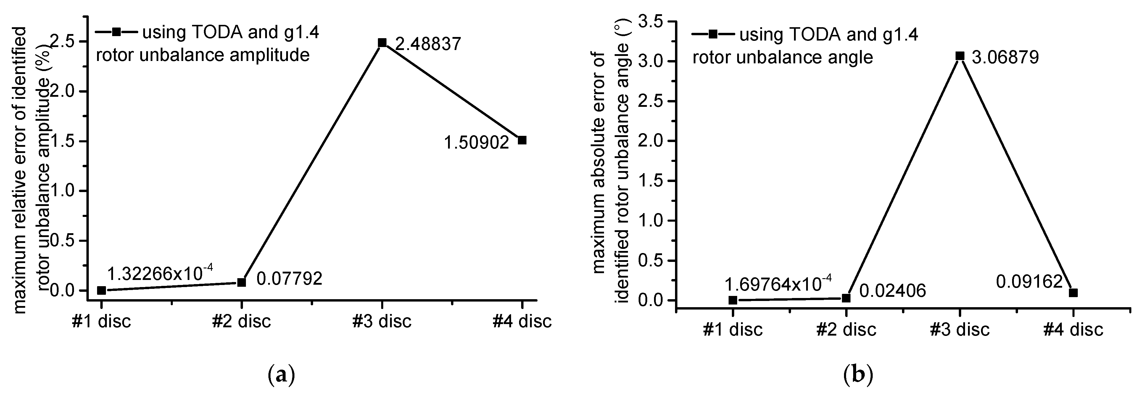
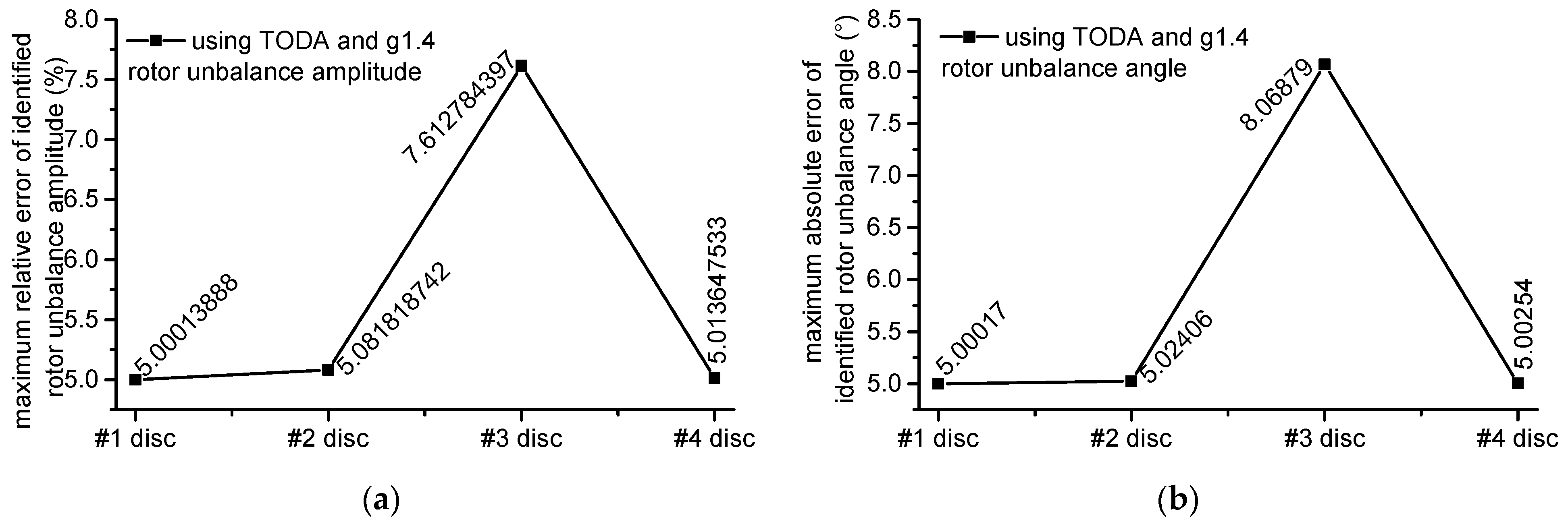
- Simulation results for rotor g1.4


Appendix B
- (1)
- Simulation results for g1.1 and h1.1
| Methods | Rotor Unbalance | G1.1 | H1.1 |
|---|---|---|---|
| SDA | Amplitude | 5.000000007 | 5.000000013 |
| Angle | 5 | 5.000000008 | |
| TODA | Amplitude | 5.000000108 | 5.000000022 |
| Angle | 5.000003329 | 5.000000025 |
- (2)
- Simulation results for rotor g1.4


- (3)
- Simulation results for rotor h4.4


Appendix C
- (1)
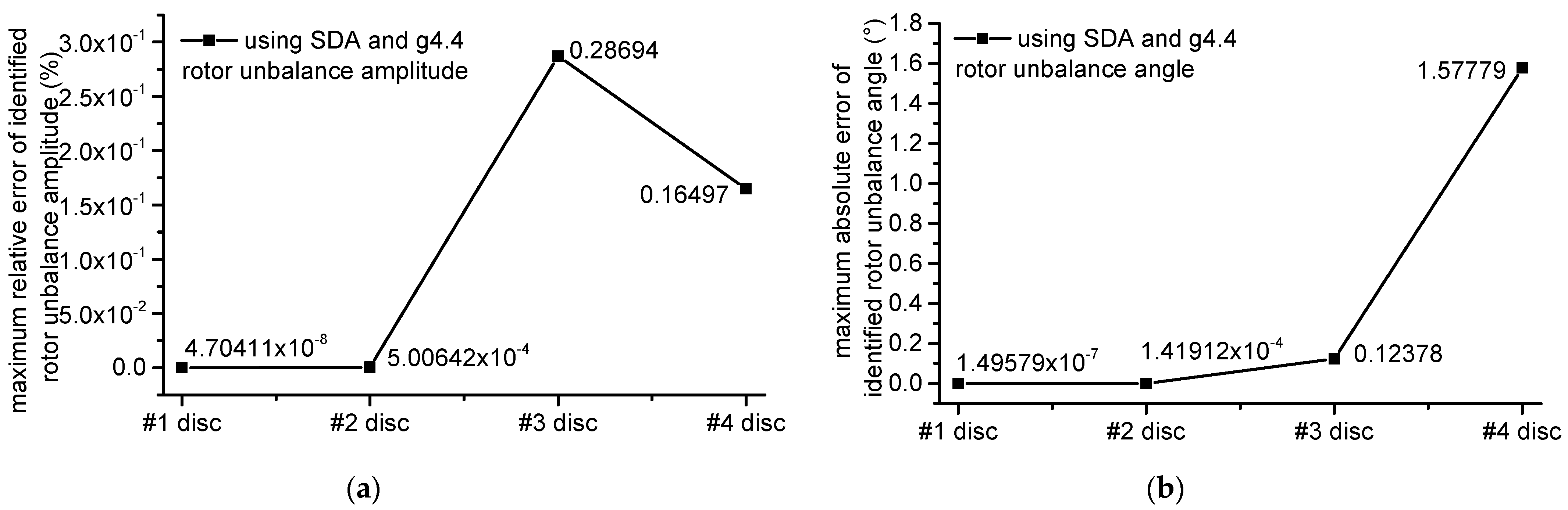
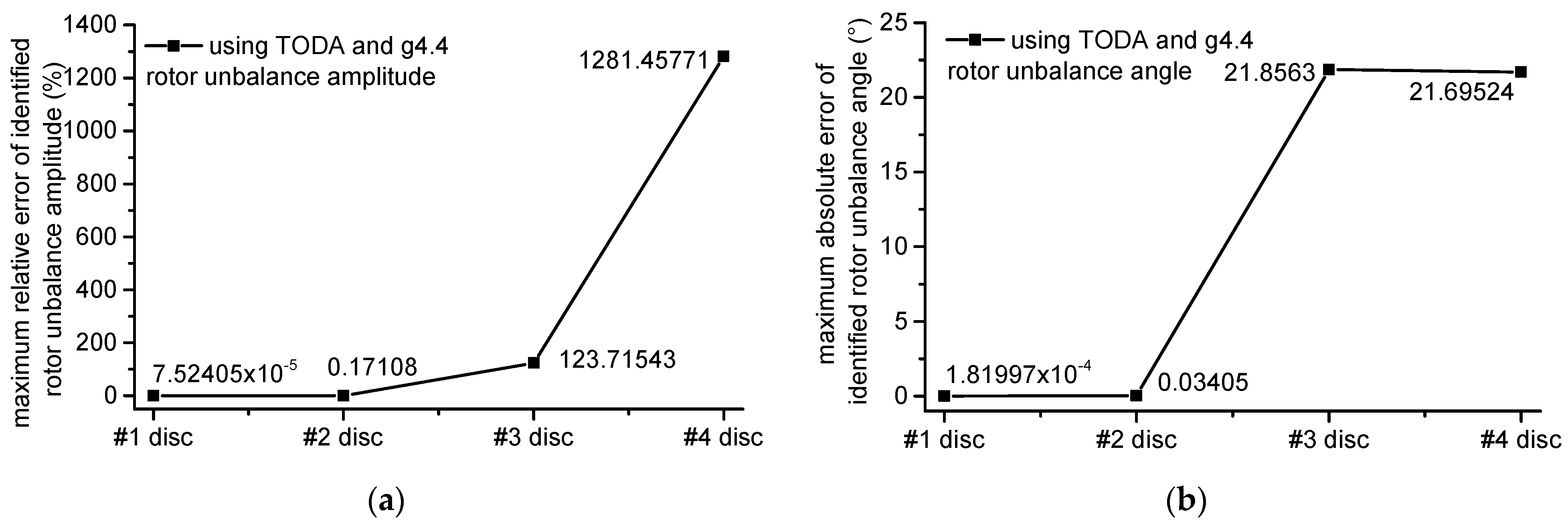
- Simulation results for g4.4


- (2)
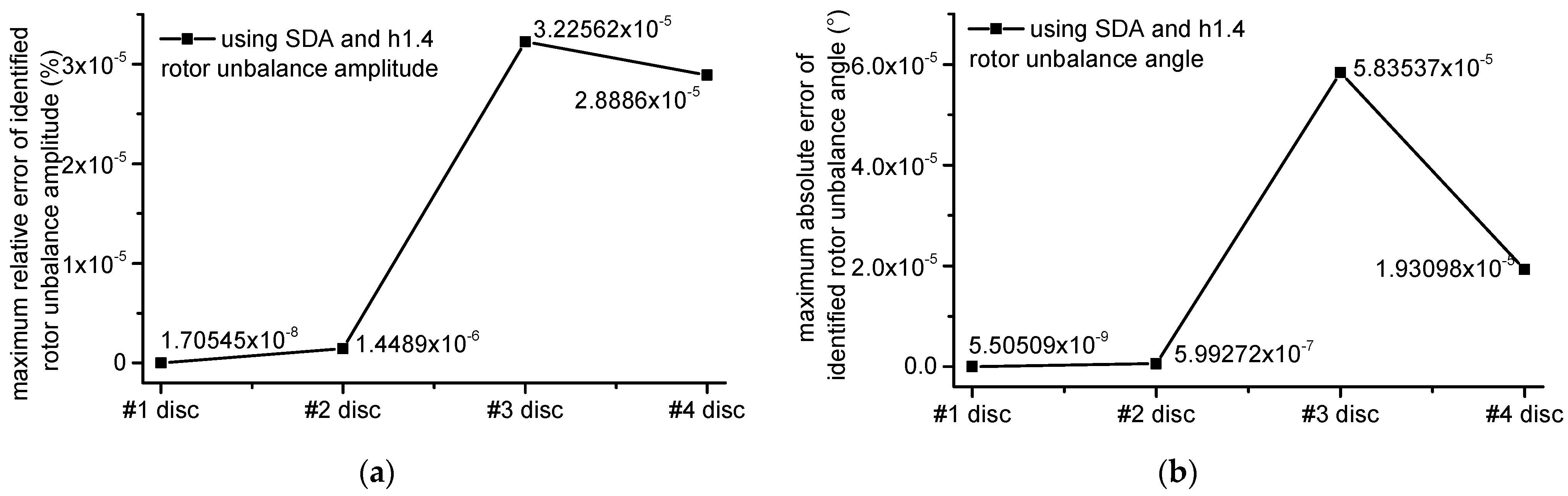
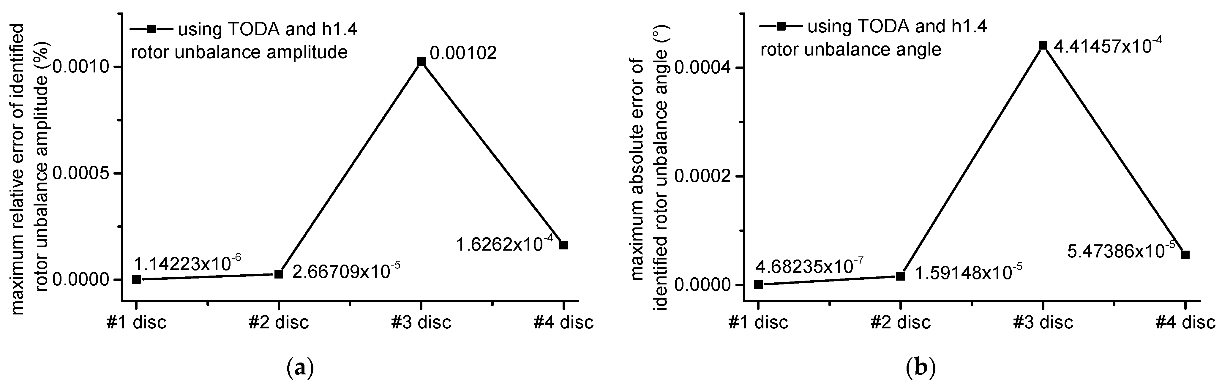
- Simulation results for h1.4


- (3)
- Simulation results for h4.4


References
- Bishop, R.E.D. The vibration of rotating shafts. J. Mech. Eng. Sci. 1959, 1, 50–65. [Google Scholar] [CrossRef]
- Gladwell, G.M.L.; Bishop, R.E.D. The vibration of rotating shafts supported in flexible bearings. J. Mech. Eng. Sci. 1959, 1, 195–206. [Google Scholar] [CrossRef]
- Goodman, T.P. A least-squares method for computing balance corrections. Trans. ASME J. Eng. Ind. 1964, 864, 273–279. [Google Scholar] [CrossRef]
- Bishop, R.E.D.; Gladwell, G.M.L. The vibration and balancing of an unbalanced flexible rotor. J. Mech. Eng. Sci. 1959, 1, 66–67. [Google Scholar] [CrossRef]
- Bishop, R.E.D.; Parkinson, A.G. On the isolation of modes in the balancing of flexible shafts. Proc. Inst. Mech. Eng. 1963, 177, 407–426. [Google Scholar]
- Lindley, A.L.G.; Bishop, R.E.D. Some recent research of the balancing of large flexible rotors. Proc. Inst. Mech. Eng. 1963, 177, 881–897. [Google Scholar] [CrossRef]
- Bishop, R.E.D.; Parkinson, A.G. On the use of balancing machines for flexible rotors. ASME J. Eng. Ind. 1972, 94, 561–576. [Google Scholar] [CrossRef]
- Kellenberger, W. Balancing flexible rotors on two generally flexible bearings. Brown Boveri Rev. 1970, 54, 603–619. [Google Scholar]
- Kellenberger, W. Should a flexible rotor be balanced in N or N + 2 planes? Trans. ASME J. Eng. Ind. 1972, 94, 548–560. [Google Scholar] [CrossRef]
- Lund, J.W.; Tonnesen, J. Analysis and experiments in multi-plane balancing of flexible rotors. Trans. ASME J. Eng. Ind. 1972, 194, 70–77. [Google Scholar] [CrossRef]
- Lund, J.W.; Tonnesen, J. Experimental and Analytic Investigation of High-Speed Rotor Balancing-Phase I; Research Report No. FR-8, Project No. FP-4; Department of Mechine Design, Technical University of Denmark: Copenhagen, Denmark, 1970. [Google Scholar]
- Shamsah, S.M.I.; Sinha, J.K.; Mandal, P. Estimating rotor unbalance from a single run-up and using reduced sensors. Measurement 2019, 136, 11–24. [Google Scholar] [CrossRef]
- Liu, Y.; Zhang, M.; Sun, C.; Hu, M.; Chen, D.; Liu, Z.; Tan, J. A method to minimize stage-by-stage initial unbalance in the aero engine assembly of multistage rotors. Aerosp. Sci. Technol. 2019, 85, 270–276. [Google Scholar] [CrossRef]
- Bin, G.; Li, X.; Shen, Y.; Wang, W. Development of whole-machine high speed balance approach for turbomachinery shaft system with N + 1 supports. Measurement 2018, 122, 368–379. [Google Scholar] [CrossRef]
- Xia, Y.; Ren, X.; Qin, W.; Yang, Y.; Lu, K.; Fu, C. Investigation on the transient response of a speed-varying rotor with sudden unbalance and its application in the unbalance identification. J. Low Freq. Noise Vib. Act. Control 2019, 39, 1065–1086. [Google Scholar] [CrossRef] [Green Version]
- Bently, D.E.; Muszynska, A. Modal testing and parameter identification of rotating shaft fluid lubricated bearing system. In Proceedings of the 4th International Conference on Modal Analysis, Orlando, FL, USA, April 1986; pp. 1393–1402. Available online: https://xueshu.baidu.com/usercenter/paper/show?paperid=635ff95826102054142b1957b8cde2db&site=xueshu_se&hitarticle=1 (accessed on 16 March 2022).
- Iida, H. Application of the Experimental Determination of Character Matrics to the Balancing of a Flexible Rotor. In Proceedings of the IFToMM 4th International Conference on Rotor Dynamics, Chicago, IL, USA, September 1994; pp. 111–115. Available online: https://xueshu.baidu.com/usercenter/paper/show?paperid=f42b876c8d2000aa6dd8baf7b534a8e8&site=xueshu_se&hitarticle=1 (accessed on 16 March 2022).
- Lou, X.; Zheng, S.; Wang, X. Some factors of leading to nonlinear electromagnetic force in active magnetic actuator. J. Mech. Electr. Eng. 1999, 2, 40–42. [Google Scholar]
- Liu, S.; Zheng, S. On-line unbalance identification of flexible rotor system. J. Zhejiang Univ. 2004, 38, 257–261. [Google Scholar]
- Shrivastava, A.; Mohanty, A.R. Estimation of single plane unbalance parameters of a rotor-bearing system using Kalman filtering based force estimation technique. J. Sound Vib. 2018, 418, 184–199. [Google Scholar] [CrossRef]
- Gillijns, S.; De Moor, B. Technical communique: Unbiased minimum-variance input and state estimation for linear discrete-time systems with direct feedthrough. Automatica 2007, 43, 934–937. [Google Scholar] [CrossRef]
- Shrivastava, A.; Mohanty, A.R. Identification of unbalance in a rotor system using a joint input-state estimation technique. J. Sound Vib. 2019, 442, 414–427. [Google Scholar] [CrossRef]
- Yao, J.; Liu, L.; Yang, F.; Scarpa, F.; Gao, J. Identification and optimization of unbalance parameters in rotor-bearing systems. J. Sound Vib. 2018, 431, 54–69. [Google Scholar] [CrossRef] [Green Version]
- Zou, D.; Zhao, H.; Liu, G.; Ta, N.; Rao, Z. Application of augmented Kalman filter to identify unbalance load of rotor-bearing system: Theory and experiment. J. Sound Vib. 2019, 463, 114972. [Google Scholar] [CrossRef]
- He, C.H.; Amer, T.S.; Tian, D.; Abolila, A.F.; Galal, A.A. Controlling the kinematics of a spring-pendulum system using an energy harvesting device. J. Low Freq. Noise Vib. Act. Control 2022. [Google Scholar] [CrossRef]
- He, J.H.; Amer, T.S.; Abolila, A.F.; Galal, A.A. Stability of three degrees-of-freedom auto-parametric system. Alex. Eng. J. 2022, 61, 8393–8415. [Google Scholar] [CrossRef]
- Wang, A.; Cheng, X.; Meng, G.; Xia, Y.; Wo, L.; Wang, Z. Dynamic analysis and numerical experiments for balancing of the continuous single-disc and single-span rotor-bearing system. Mech. Syst. Signal Process. 2017, 86, 151–176. [Google Scholar] [CrossRef]
- Tiwari, R.; Chakravarthy, V. Simultaneous estimation of the residual unbalance and bearing dynamic parameters from the experimental data in a rotor-bearing system. Mech. Mach. Theory 2009, 44, 792–812. [Google Scholar] [CrossRef]
- Tiwari, R. Conditioning of regression matrices for simultaneous estimation of the residual unbalance and bearing dynamic parameters. Mech. Syst. Signal Process. 2005, 19, 1082–1095. [Google Scholar] [CrossRef]
- Wang, A.; Yao, W.; He, K.; Meng, G.; Cheng, X.; Yang, J. Analytical modelling and numerical experiment for simultaneous identification of unbalance and rolling-bearing coefficients of the continuous single-disc and single-span rotor-bearing system with Rayleigh beam model. Mech. Syst. Signal Process. 2019, 116, 322–346. [Google Scholar] [CrossRef]
- Jamadar, I.M. A Model to Estimate Synchronous Vibration Amplitude for Detection of Unbalance in Rotor-Bearing System. Int. J. Acoust. Vib. 2021, 26, 161–169. [Google Scholar] [CrossRef]
- Ambur, R.; Rinderknecht, S. Unbalance detection in rotor systems with active bearings using self-sensing piezoelectric actuators. Mech. Syst. Signal Process. 2018, 102, 72–86. [Google Scholar] [CrossRef]
- Sanches, F.D.; Pederiva, R. Simultaneous identification of unbalance and shaft bow in a two-disk rotor based on correlation analysis and the SEREP model order reduction method. J. Sound Vib. 2018, 433, 230–247. [Google Scholar] [CrossRef]
- Zhang, Y.; Li, M.; Yao, H.; Gou, Y.; Wang, X. A modal-based balancing method for a high-speed rotor without trial weights. Mech. Sci. 2021, 12, 85–96. [Google Scholar] [CrossRef]
- Tiwari, R.; Chakravarthy, V. Simultaneous identification of residual unbalances and bearing dynamic parameters from impulse responses of rotor–bearing systems. Mech. Syst. Signal Process. 2006, 20, 1590–1614. [Google Scholar] [CrossRef]
- Tiwari, R.; Chakravarthy, V. Identification of the bearing and unbalance parameters from rundown data of rotors. In IUTAM Symposium on Emerging Trends in Rotor Dynamics; Springer: Dordrecht, The Netherlands, 2011; pp. 479–489. [Google Scholar]


| Parameter | Meaning |
|---|---|
| r_shaft | Radius of the shaft |
| p_shaft | Density of the shaft |
| E_shaft | Elastic modulus of the shaft |
| L_shaft | Length of the shaft |
| r_disc | Radius of the disc |
| p_disc | Density of the disc |
| E_disc | Elastic modulus of the disc |
| L_disc | Width of the disc |
| Parameter | Value | Parameter | Value |
|---|---|---|---|
| r_shaft of rotor g1.1, g1.4 and g4.4 | 10 × 10−3 m | L_shaft of the rotor g1.4 | 1200 × 10−3 m |
| r_shaft of rotor h1.1, h1.4 and h4.4 | 15 × 10−3 m | L_shaft of the rotor g4.4 | 1600 × 10−3 m |
| p_shaft | 7800 kgm−3 | L_shaft of the rotor h1.1 | 1400 × 10−3 m |
| E_shaft | 2.1 × 10¹¹ Pa | L_shaft of the rotor h1.4 | 1400 × 10−3 m |
| L_shaft of the rotor g1.1 | 800 × 10−3 m | L_shaft of the rotor h4.4 | 3600 × 10−3 m |
| Parameter | Value | Parameter | Value | Parameter | Value |
|---|---|---|---|---|---|
| 0.12031 kg | 0.15 kg | 0.01 kg | |||
| 50 × 10−3 m | 10 × 10−3 m | 20 × 10−3 m | |||
| 225° | 120° | −120° | |||
| 0.10 kg | r_disc of #1 disc | 60 × 10−3 m | p_disc of of #1~#4 disc | 7800 kgm−3 | |
| 15 × 10−3 m | r_disc of #2~#4 | 50 × 10−3 m | E_disc of of #1~#4 disc | 2.1 × 10¹¹ Pa | |
| −170° | L_disc of of #1~#4 disc | 10 × 10−3 m |
| Parameter | Value | Parameter | Value | Parameter | Value |
|---|---|---|---|---|---|
| 0.05 kg | 0.15 kg | 0.01 kg | |||
| 30 × 10−3 m | 10 ×10−3 m | 20 × 10−3 m | |||
| 45° | 90° | 170° | |||
| 0.10 kg | r_disc of #1–4 disc | 50 × 10−3 m | p_disc of of #1~#4 disc | 7800 kgm−3 | |
| 15 × 10−3 m | L_disc of of #1~#4 disc | 10 × 10−3 m | |||
| −170° | E_disc of of #1~#4 disc | 2.1 × 10¹¹ Pa |
| Parameter | Value | Parameter | Value |
|---|---|---|---|
| N/m | N/m | ||
| N·s/m | N·s/m | ||
| N/m | N/m | ||
| N·s/m | N·s/m | ||
| N/m | N/m | ||
| N·s/m | N·s/m | ||
| N/m | N/m | ||
| N·s/m | N·s/m |
| Parameter | Value | Parameter | Value |
|---|---|---|---|
| N/m | = 2 to 8 | N/m | |
| , | N·s/m | = 2 to 8 | N·s/m |
| Disc | Unbalance | Value | Value | Value | Value |
|---|---|---|---|---|---|
| #1 | Amplitude | (10.84%, 1 Hz) | - | - | - |
| Angle | - | - | - | - | |
| #2 | Amplitude | - | - | (42.54%, 645 Hz) | - |
| Angle | - | - | - | - | |
| #3 | Amplitude | (26.02%, 1 Hz) | (257.24%, 269 Hz) | - | (20.64%, 1265 Hz) |
| Angle | (19.49°, 1 Hz) | - | (11.72°, 645 Hz) | - | |
| #4 | Amplitude | - | - | - | - |
| Angle | - | (16.259°, 269 Hz) | - | - |
| Disc | Unbalance | Value | Value | Value | Value |
|---|---|---|---|---|---|
| #1 | Amplitude | (83.36%, 1 Hz) | - | - | - |
| Angle | - | - | - | - | |
| #2 | Amplitude | (95.6%, 1 Hz) | (42.54%, 269 Hz) | - | - |
| Angle | (32.5°, 1 Hz) | - | - | - | |
| #3 | Amplitude | (242.24%, 1 Hz) | (257.24%, 269 Hz) | (11.64%, 645 Hz) | (20.64%, 1265 Hz) |
| Angle | (108.42°, 1 Hz) | (57.41°, 271 Hz) | (11.72°, 645 Hz) | - | |
| #4 | Amplitude | - | - | - | - |
| Angle | (165.08°, 1 Hz) | (16.259°, 269 Hz) | - | - |
| Disc | Unbalance | Value | Value | Value | Value |
|---|---|---|---|---|---|
| #1 | Amplitude | (695.26%, 4 Hz) | (19.45%, 268 Hz) | - | - |
| Angle | (140.04°, 4 Hz) | (10.86°, 268 Hz) | - | - | |
| #2 | Amplitude | (597.53%, 4 Hz) | (22.7%, 270 Hz) | - | - |
| Angle | (94.44°, 4 Hz) | - | - | - | |
| #3 | Amplitude | (1722.04%, 8 Hz) | (262.49%, 268 Hz) | - | (11.76%, 1268 Hz) |
| Angle | (120.31°, 16 Hz) | (20.6°, 270 Hz) | - | (11.3°, 1268 Hz) | |
| #4 | Amplitude | (853.26%, 6 Hz) | - | - | - |
| Angle | (165.1°, 10 Hz) | (10.04°, 270 Hz) | - | - |
| Disc | Unbalance | Value |
|---|---|---|
| #1 disc | Amplitude | - |
| Angle | - | |
| #2 disc | Amplitude | - |
| Angle | - | |
| #3 disc | Amplitude | (11.73%, 1264 Hz) |
| Angle | (11.56°, 1268 Hz) | |
| #4disc | Amplitude | - |
| Angle | - |
| First Order | Second Order | Third Order |
|---|---|---|
| 269 Hz | 645 Hz | 1267 Hz |
| Sensor Resolution | Low Frequency (1 Hz) | First Order (269 Hz) | Second Order (645 Hz) | Third Order (1267 Hz) |
|---|---|---|---|---|
| 0.1 nm | (10.84%, 1 Hz) | (2.02%, 271 Hz) | (0.31%, 643 Hz) | (0.42%, 1267 Hz) |
| (2.12°, 1 Hz) | (1.47°, 271 Hz) | (0.32°, 645 Hz) | (0.32°, 1267 Hz) | |
| 1 nm | (83.36%, 1 Hz) | (1.92%, 269 Hz) | (0.31%, 643 Hz) | (0.42%, 1267 Hz) |
| (8.77°, 1 Hz) | (1.45°, 271 Hz) | (0.32°, 645 Hz) | (0.32°, 1267 Hz) | |
| 0.1 um | (695.26%, 4 Hz) | (19.45%, 268 Hz) | (0.65%, 646 Hz) | (0.62%, 1266 Hz) |
| (140.04°, 4 Hz) | (10.86°, 268 Hz) | (0.55°, 646 Hz) | (0.45°, 1262 Hz) | |
| 1 um | Cannot be identified | Cannot be identified | Cannot be identified | (0.63%, 1266 Hz) |
| Cannot be identified | Cannot be identified | Cannot be identified | (0.45°, 1262 Hz) |
Publisher’s Note: MDPI stays neutral with regard to jurisdictional claims in published maps and institutional affiliations. |
© 2022 by the authors. Licensee MDPI, Basel, Switzerland. This article is an open access article distributed under the terms and conditions of the Creative Commons Attribution (CC BY) license (https://creativecommons.org/licenses/by/4.0/).
Share and Cite
Wang, A.; Bi, Y.; Feng, Y.; Yang, J.; Cheng, X.; Meng, G. Continuous Rotor Dynamics of Multi-Disc and Multi-Span Rotors: A Theoretical and Numerical Investigation of the Identification of Rotor Unbalance from Unbalance Responses. Appl. Sci. 2022, 12, 3865. https://doi.org/10.3390/app12083865
Wang A, Bi Y, Feng Y, Yang J, Cheng X, Meng G. Continuous Rotor Dynamics of Multi-Disc and Multi-Span Rotors: A Theoretical and Numerical Investigation of the Identification of Rotor Unbalance from Unbalance Responses. Applied Sciences. 2022; 12(8):3865. https://doi.org/10.3390/app12083865
Chicago/Turabian StyleWang, Aiming, Yujie Bi, Yu Feng, Jie Yang, Xiaohan Cheng, and Guoying Meng. 2022. "Continuous Rotor Dynamics of Multi-Disc and Multi-Span Rotors: A Theoretical and Numerical Investigation of the Identification of Rotor Unbalance from Unbalance Responses" Applied Sciences 12, no. 8: 3865. https://doi.org/10.3390/app12083865