
Adaptive, Observer-Based Synchronization of Different Chaotic Systems


Abstract
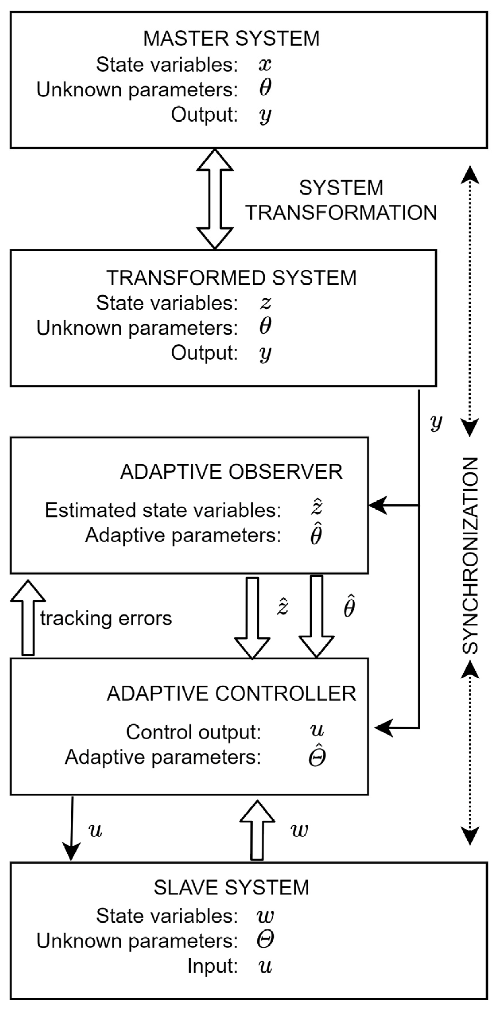
:1. Introduction
- Master and slave systems may be different;
- Master and slave systems contain (different) unknown, constant parameters;
- Only the single output of the master system is available;
- The slave system is controlled by a single input located in the last state equation.
2. Adaptive Observer for an Output Nonlinear Parametric System
- The matrix variable is an output of a linear filter to be defined;
- The unknown parameters are substituted by adaptive parameters , tuned according to adaptive lawwhere ; is a symmetric, positive definite matrix of design parameters;
- The component and the tuning function are used to modify the observer dynamics according to the slave system tracking errors, and meanwhile may be assumed equal to zero.
3. Master Chaotic Systems Transformable into ONP Form
4. Slave System
5. Adaptive Control
5.1. STAGE 1
5.2. STAGE 2
5.3. STAGE 3
6. Closed-Loop System Stability
7. Example
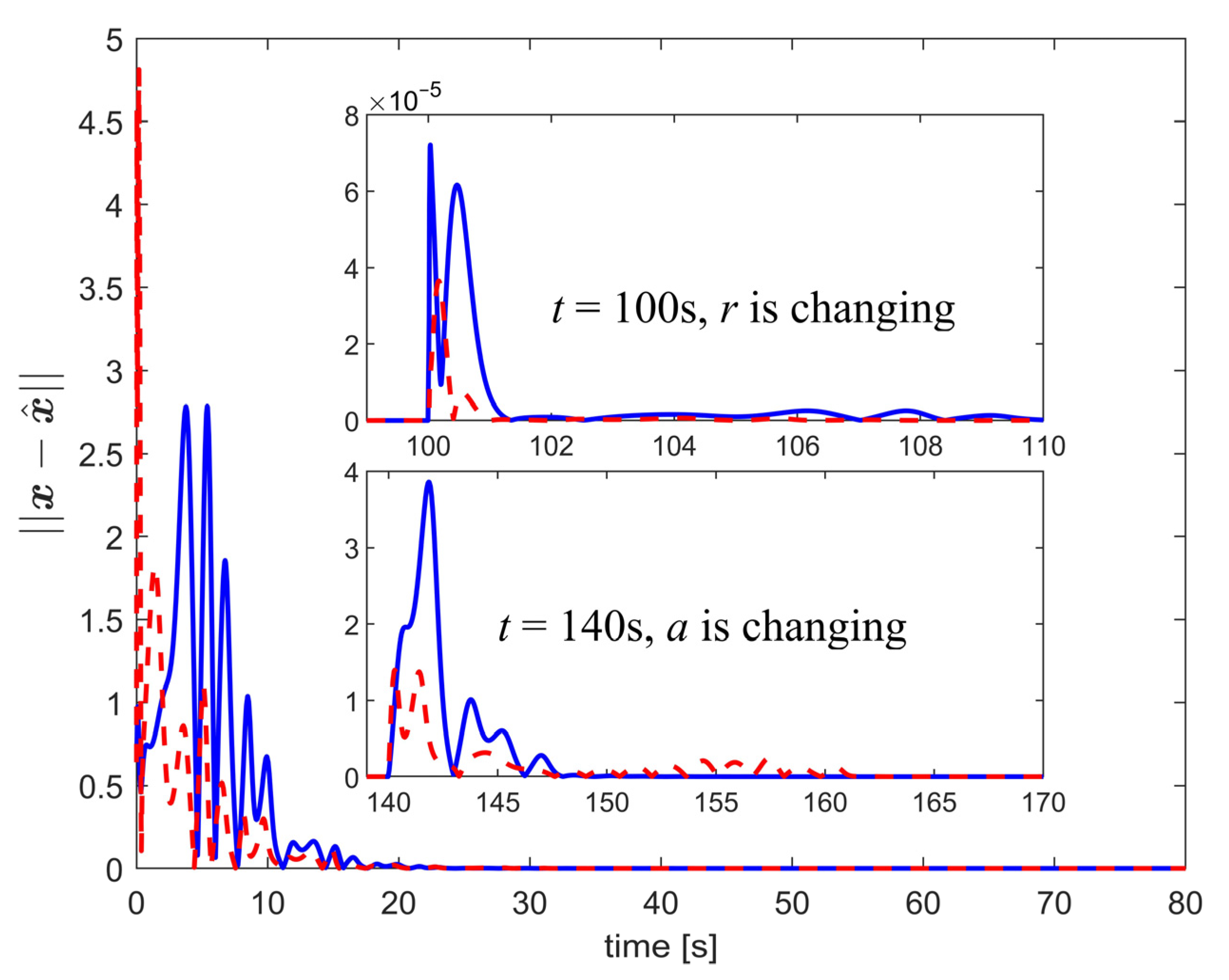
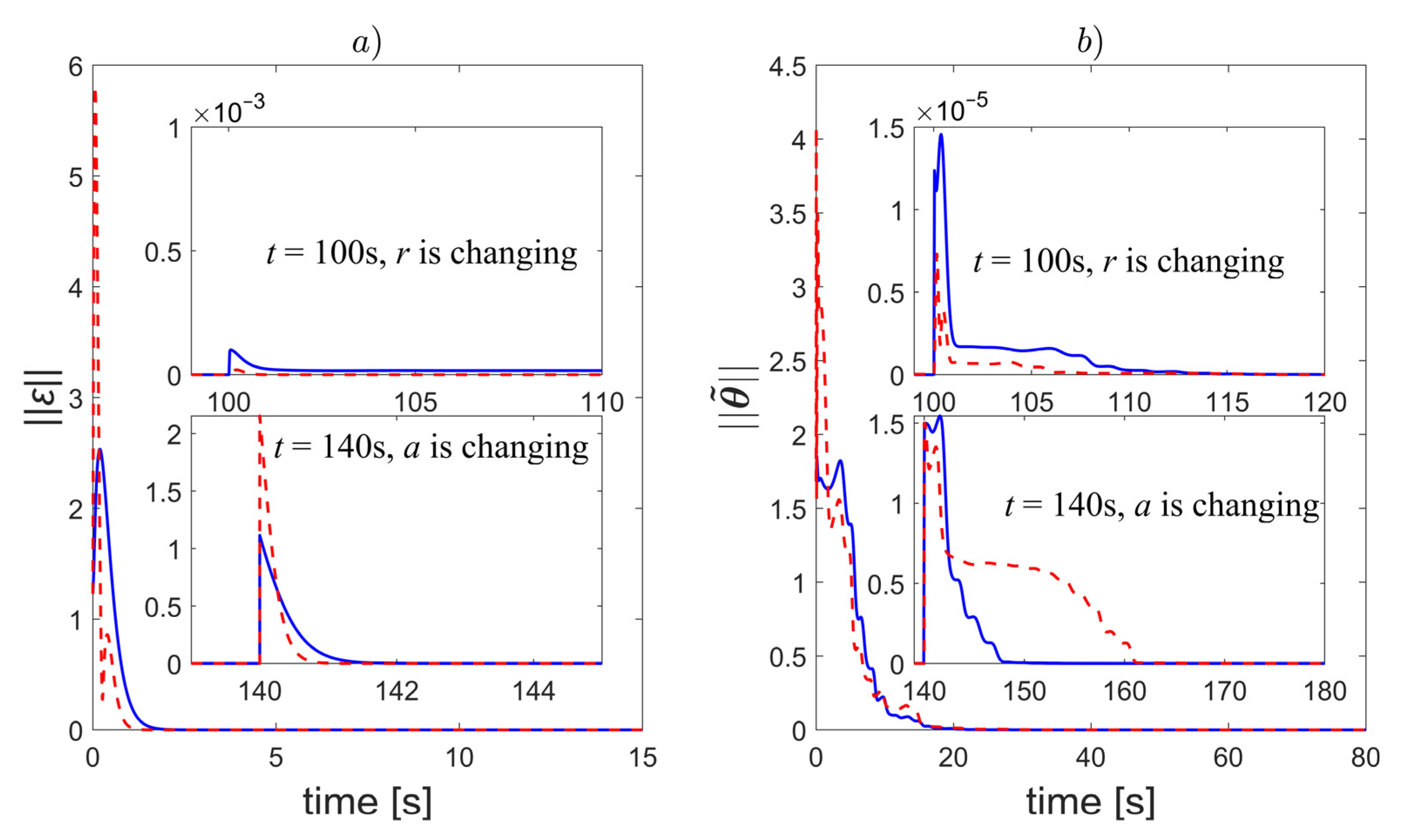
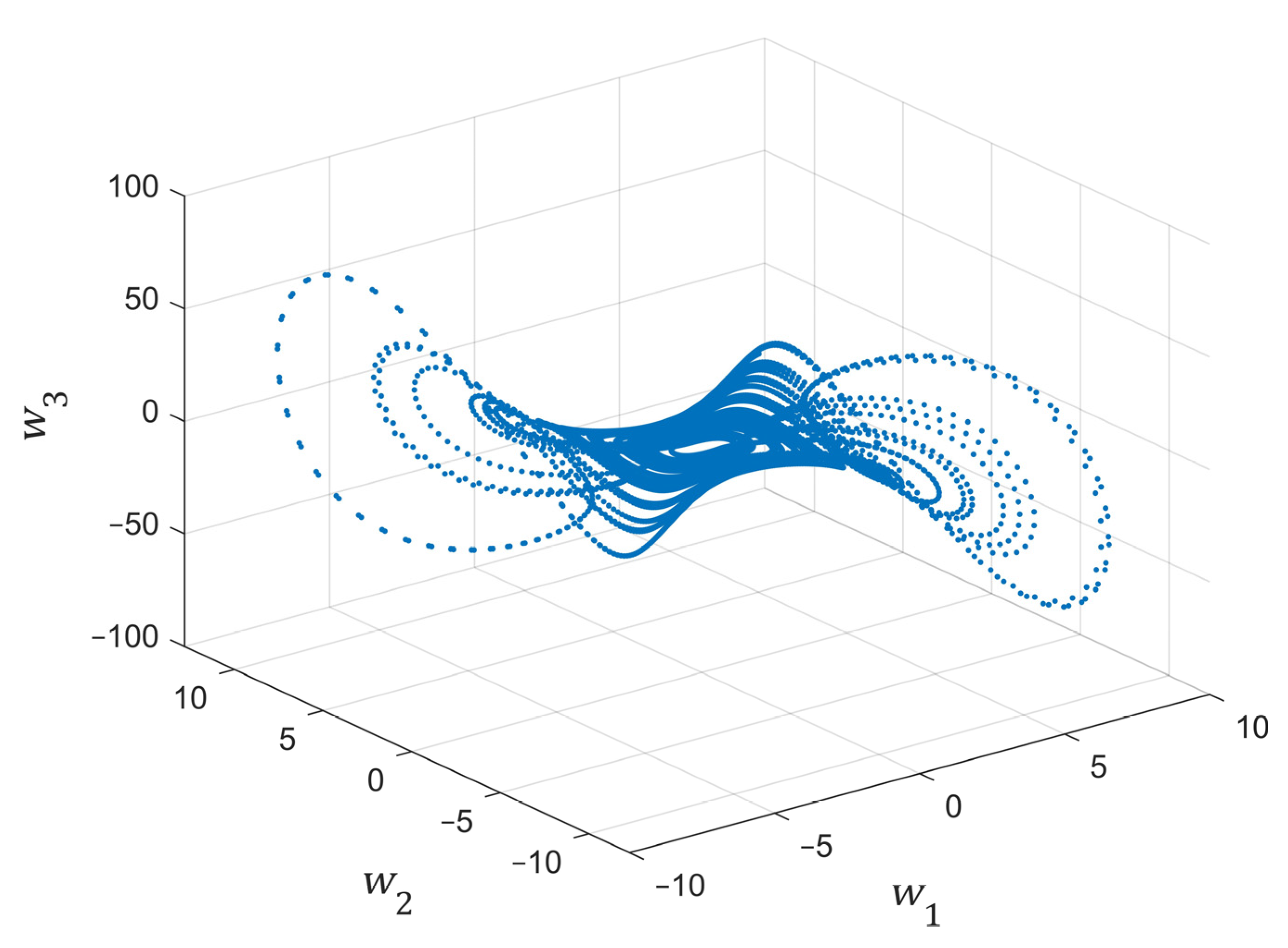
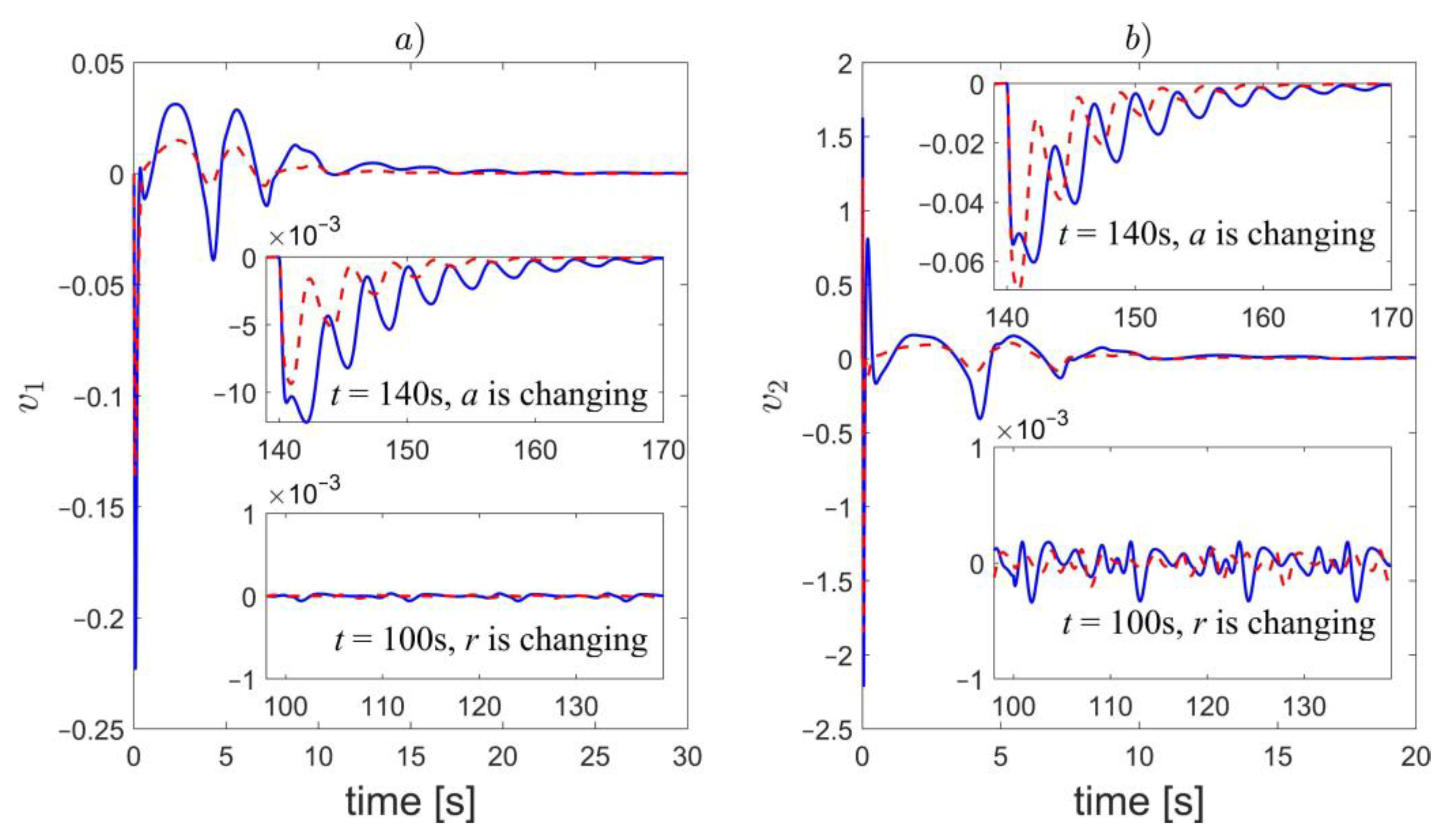
7.1. Example 1—Observer Performance
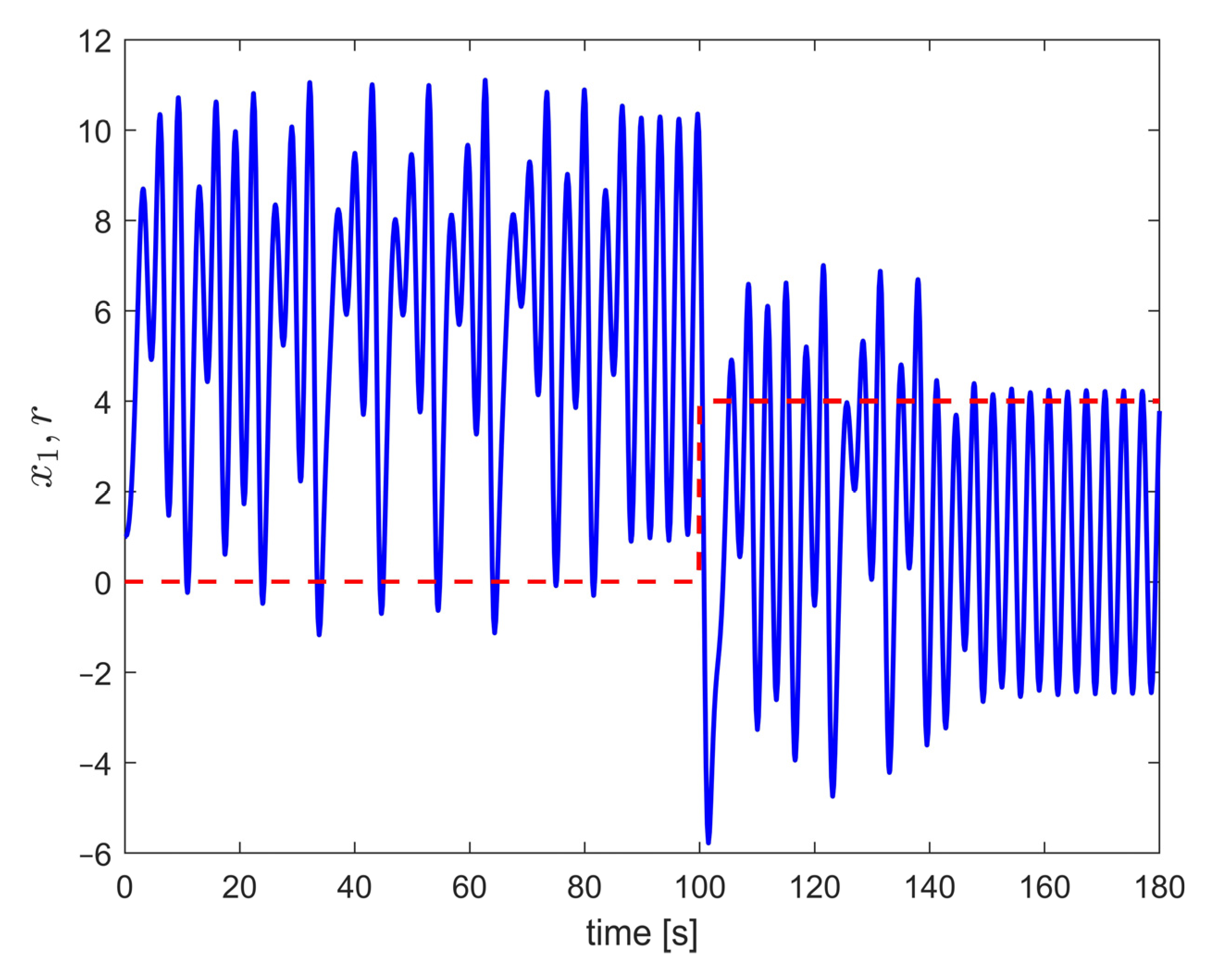
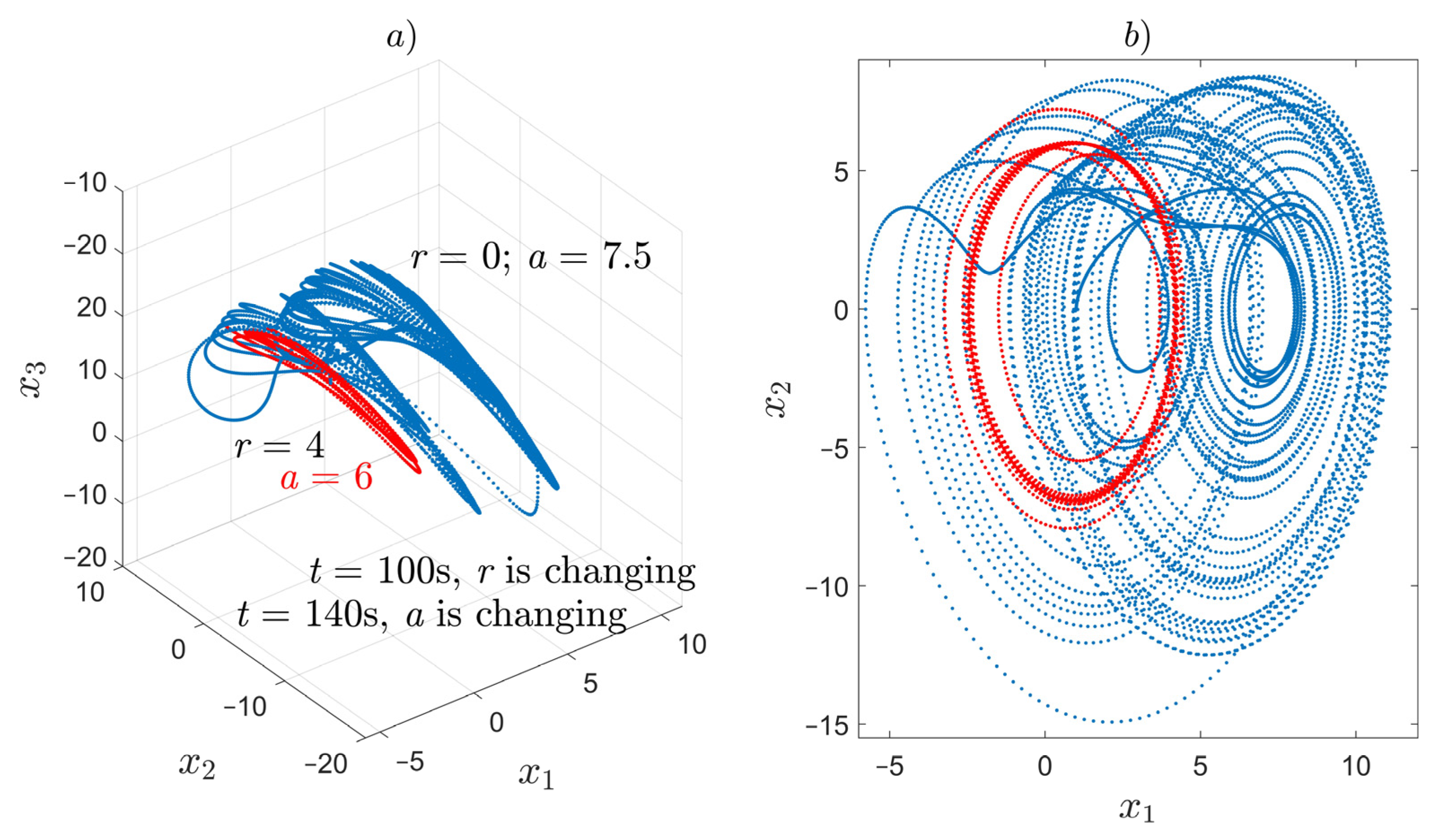
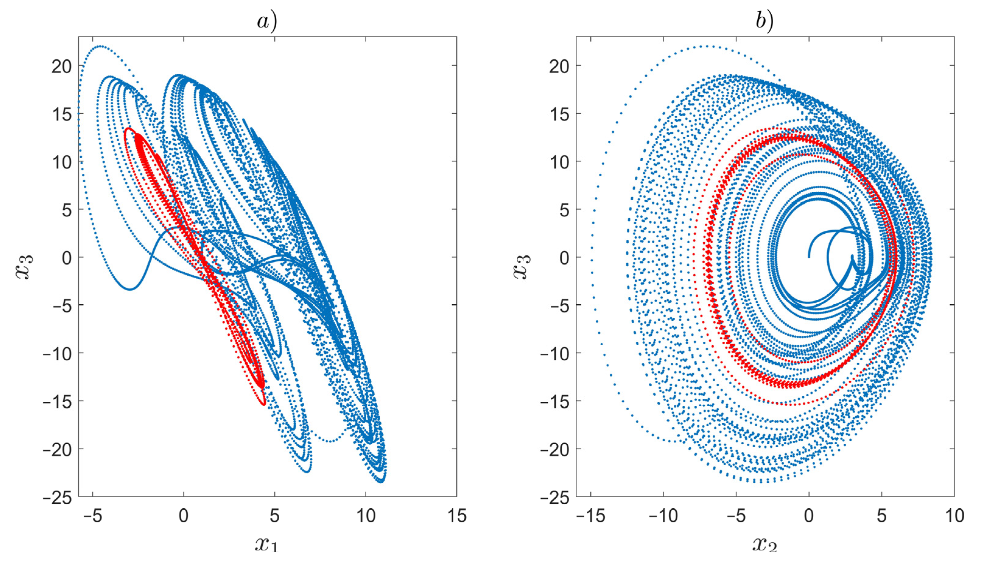
7.2. Example 2—Synchronization
8. Conclusions
Author Contributions
Funding
Institutional Review Board Statement
Informed Consent Statement
Data Availability Statement
Conflicts of Interest
Appendix A
References
- Pecora, L.M.; Carroll, T.L. Synchronization in Chaotic Systems. Phys. Rev. Lett. 1990, 64, 821–824. [Google Scholar] [CrossRef]
- Kun, G. A Synchronization Controller for the Unified Chaotic System and Its Application in Secure Communication. In Proceedings of the 2011 International Conference on Consumer Electronics, Communications and Networks (CECNet), Xianning, China, 11–13 March 2011; pp. 4700–4703. [Google Scholar]
- Lin, X.; Zhou, S.; Zou, Z.; Li, Y. Chaos and Its Communication Application of Fractional-Order Neutral Differential System. In Proceedings of the 2010 International Workshop on Chaos-Fractal Theories and Applications, Kunming, China, 29–31 October 2010; pp. 174–178. [Google Scholar]
- Yang, L.; Zhang, J. A New Multistage Chaos Synchronized System for Secure Communications and Noise Perturbation. In Proceedings of the 2009 International Workshop on Chaos-Fractals Theories and Applications, Shenyang, China, 6–8 November 2009; pp. 35–39. [Google Scholar]
- Koltsova, E.M.; Cherenkov, M.V.; Korchagin, E.Y. Nonlinear Processes and Control of Chaos in Chemical Technology. In Proceedings of the 2003 IEEE International Workshop on Workload Characterization, Austin, TX, USA, 27 October 2003; Volume 2, pp. 484–490. [Google Scholar]
- Frisman, E.Y.; Sycheva, E.V. Oscillations and Chaos in Population Dynamics Caused by Hunting. In Proceedings of the 2000 2nd International Conference. Control of Oscillations and Chaos, Saint Petersburg, Russia, 5–7 July 2000; Volume 3, pp. 576–578. [Google Scholar]
- Ji, W. Chaos and Control of Nonlinear Dynamic Model in the Ecological System. In Proceedings of the 2010 International Workshop on Chaos-Fractal Theories and Applications, Kunming, China, 29–31 October 2010; pp. 326–330. [Google Scholar]
- Gómez-Pavón, L.C.; Muñoz-Pacheco, J.M.; Luis-Ramos, A. Synchronous Chaos Generation in an Er3+-Doped Fiber Laser System. IEEE Photonics J. 2015, 7, 1–6. [Google Scholar] [CrossRef]
- Roy, R. Coherence and Chaos in Solid State Laser Systems. In Proceedings of the LEOS ’95. IEEE Lasers and Electro-Optics Society 1995 Annual Meeting. 8th Annual Meeting, San Francisco, CA, USA, 30–31 October 1995; Volume 1, pp. 155–156. [Google Scholar]
- Zhang, H.; Huang, W.; Wang, Z.; Chai, T. Adaptive Synchronization between Two Different Chaotic Systems with Unknown Parameters. Phys. Lett. A 2006, 350, 363–366. [Google Scholar] [CrossRef]
- Kabziński, J. Synchronization of an Uncertain Duffing Oscillator with Higher Order Chaotic Systems. Int. J. Appl. Math. Comput. Sci. 2018, 28, 625–634. [Google Scholar] [CrossRef] [Green Version]
- Guo, J.; Zhao, Z.; Shi, F.; Wang, R.; Li, S. Observer-Based Synchronization Control for Coronary Artery Time-Delay Chaotic System. IEEE Access 2019, 7, 51222–51235. [Google Scholar] [CrossRef]
- Cui, D.; Xu, J. Synchronization of Chaotic Systems Having Triangular Structure via Observer. In Proceedings of the 2018 37th Chinese Control Conference (CCC), Wuhan, China, 25–27 July 2018; pp. 769–773. [Google Scholar]
- Kocamaz, U.E.; Uyaroğlu, Y.; Kizmaz, H. Control of Rabinovich Chaotic System Using Sliding Mode Control. Int. J. Adapt. Control Signal Processing 2014, 28, 1413–1421. [Google Scholar] [CrossRef]
- Vaidyanathan, S.; Rasappan, S. Global Chaos Synchronization of N-Scroll Chua Circuit and Lur’e System Using Backstepping Control Design with Recursive Feedback. Arab. J. Sci. Eng. 2014, 39, 3351–3364. [Google Scholar] [CrossRef]
- Singh, S.; Handa, H. Synchronization of MLS Chaotic System Using Adaptive Backstepping Control. In Proceedings of the 2020 7th International Conference on Signal Processing and Integrated Networks (SPIN), 27–28 February 2020; pp. 1084–1088. [Google Scholar]
- Shukla, M.; Bansal, A.; Sharma, B.B. Synchronization of a Class of Non-Identical Chaotic Systems via DSC Approach. In Proceedings of the 2013 IEEE International Conference on Signal Processing, Computing and Control (ISPCC), Waknaghat, India, 26–28 September 2013; pp. 1–6. [Google Scholar]
- Li, D.-J. Adaptive Output Feedback Control of Uncertain Nonlinear Chaotic Systems Based on Dynamic Surface Control Technique. Nonlinear Dyn. 2012, 68, 235–243. [Google Scholar] [CrossRef]
- Zhang, J.; Cui, Q.; Zhao, Z.; Huo, S. Synchronization Control Design Based On Observers For Time-Delay Lur’e Systems. IEEE Access 2020, 8, 92886–92894. [Google Scholar] [CrossRef]
- Cui, D.; Zhu, H.; Liu, H. Adaptive Fuzzy Control for a Class of Uncertain Chaotic Systems Based on Proportional-Integral Sliding Mode Control Approach. In Proceedings of the 2018 Chinese Control And Decision Conference (CCDC), Shenyang, China, 9–11 June 2018; pp. 589–593. [Google Scholar]
- N’Doye, I.; Darouach, M.; Voos, H. Observer-Based Approach for Fractional-Order Chaotic Synchronization and Communication. In Proceedings of the 2013 European Control Conference (ECC), Zurich, Switzerland, 17–19 July 2013; pp. 4281–4286. [Google Scholar]
- Borri, A.; Cacace, F.; Gaetano, A.; de Germani, A.; Manes, C.; Palumbo, P.; Panunzi, S.; Pepe, P. Luenberger-Like Observers for Nonlinear Time-Delay Systems with Application to the Artificial Pancreas: The Attainment of Good Performance. IEEE Control Syst. 2017, 37, 33–49. [Google Scholar] [CrossRef]
- Guay, M. Adaptive Gain Nonlinear Observer Design Techniques. In Proceedings of the 2017 6th International Symposium on Advanced Control of Industrial Processes (AdCONIP), Taipei, Taiwan, 28–31 May 2017; pp. 143–148. [Google Scholar]
- Kazantzis, N.; Kravaris, C. A Nonlinear Luenberger-Type Observer with Application to Catalyst Activity Estimation. In Proceedings of the 1995 American Control Conference - ACC’95; American Autom Control Council, Seattle, WA, USA, 21–23 June 1995; Volume 3, pp. 1756–1761. [Google Scholar]
- Chernikova, O.S. An Adaptive Unscented Kalman Filter Approach for State Estimation of Nonlinear Continuous-Discrete System. In Proceedings of the 2018 XIV International Scientific-Technical Conference on Actual Problems of Electronics Instrument Engineering (APEIE), Novosibirsk, Russia, 2–6 October 2018; pp. 37–40. [Google Scholar]
- Fei, J.; Hua, M. A Novel Design of Adaptive Sliding Mode Observer. In Proceedings of the 2010 8th World Congress on Intelligent Control and Automation, Jinan, China, 6–9 July 2010; pp. 843–848. [Google Scholar]
- Vo, A.T.; Kang, H.-J.; Nguyen, V.-C. An Output Feedback Tracking Control Based on Neural Sliding Mode and High Order Sliding Mode Observer. In Proceedings of the 2017 10th International Conference on Human System Interactions (HSI), Ulsan, Korea, 17–19 July 2017; pp. 161–165. [Google Scholar]
- Saad, M.; Liaquat, M. Output Regulation of Feedback Linearizable System (Single Link Robot Manipulator): A Cascaded High Gain Observer Approach. In Proceedings of the 2017 7th IEEE International Conference on Control System, Computing and Engineering (ICCSCE), Penang, Malaysia, 24–26 November 2017; pp. 226–229. [Google Scholar]
- Khalil, H.K. Cascade High-Gain Observer for High-Dimensional Systems. In Proceedings of the 2016 IEEE 55th Conference on Decision and Control (CDC), Las Vegas, NV, USA, 12–14 December 2016; pp. 7141–7146. [Google Scholar]
- Wang, H.; Dong, Y.; Qin, W. Adaptive Observer Design for a Class of Lipschitz Nonlinear Systems. In Proceedings of the Proceedings of the 30th Chinese Control Conference, Yantai, China, 22–24 July 2011; pp. 665–669.
- Hu, G.-D. Observers for One-Sided Lipschitz Non-Linear Systems. IMA J. Math. Control Inf. 2006, 23, 395–401. [Google Scholar] [CrossRef]
- Zhao, Y.; Zhang, W.; Su, H.; Yang, J. Observer-Based Synchronization of Chaotic Systems Satisfying Incremental Quadratic Constraints and Its Application in Secure Communication. IEEE Trans. Syst. Man Cybern. Syst. 2020, 50, 5221–5232. [Google Scholar] [CrossRef]
- Krstic, M.; Ioannis, K.; Kokotovic, P.V. Nonlinear and Adaptive Control Design; Wiley: New York, NY, USA, 1995; ISBN 978-0-471-12732-1. [Google Scholar]
- Kreisselmeier, G. Adaptive Observers with Exponential Rate of Convergence. IEEE Trans. Autom. Control 1977, 22, 2–8. [Google Scholar] [CrossRef]
- Zhu, F.; Xu, J.; Chen, M. The Combination of High-Gain Sliding Mode Observers Used as Receivers in Secure Communication. IEEE Trans. Circuits Syst. I: Regul. Pap. 2012, 59, 2702–2712. [Google Scholar] [CrossRef]
- Gao, Y.-F.; Sun, X.-M.; Wen, C.; Wang, W. Observer-Based Adaptive NN Control for a Class of Uncertain Nonlinear Systems With Nonsymmetric Input Saturation. IEEE Trans. Neural Netw. Learn. Syst. 2017, 28, 1520–1530. [Google Scholar] [CrossRef] [PubMed]
- Kabziński, J.; Mosiołek, P. Projektowanie Nieliniowych Układów Sterowania (Nonlinear Control Design), 1st ed.; PWN SA: Warszawa, Poland, 2018; ISBN 978-83-01-19697-4. [Google Scholar]
- Vaidyanathan, S. Output Regulation of Arneodo-Coullet Chaotic System. In Proceedings of the Advanced Computing; Meghanathan, N., Kaushik, B.K., Natarajan, D., Eds.; Springer Berlin Heidelberg: Berlin, Heidelberg, 2011; pp. 98–107. [Google Scholar]
- Park, J.H. Synchronization of Genesio Chaotic System via Backstepping Approach. Chaos Solitons Fractals 2006, 27, 1369–1375. [Google Scholar] [CrossRef]
- Mazenc, F.; Praly, L.; Dayawansa, W.P. Global Stabilization by Output Feedback: Examples and Counterexamples. Syst. Control Lett. 1994, 23, 119–125. [Google Scholar] [CrossRef]
- Ioannou, P.; Sun, J. Robust Adaptive Control; DOVER PUBN INC.: New York, NY, USA, 2012; ISBN 978-0-486-49817-1. [Google Scholar]
- Sastry, S.; Bodson, M. Adaptive Control: Stability, Convergence, and Robustness; Prentice Hall: Englewood Cliffs, NJ, USA, 1989; ISBN 0130043265. [Google Scholar]
- Marino, R. Adaptive Observers for Single Output Nonlinear Systems. IEEE Trans. Autom. Control 1990, 35, 1054–1058. [Google Scholar] [CrossRef]
- Vaidyanathan, S. A New 3-D Jerk Chaotic System with Two Cubic Nonlinearities and Its Adaptive Backstepping Control. Arch. Control Sci. 2017, 27, 409–439. [Google Scholar] [CrossRef]


| Adaptive Observer | Adaptive Controller | ||
|---|---|---|---|
| Estimated state variables | Synchronization error, first-loop tracking error | ||
| Estimation error | First-loop stabilizing function (desired trajectory for | ||
| First-state variable estimation error | Tracking error for | ||
| “Composite” error | Second-loop stabilizing function (desired trajectory for | ||
| Adaptive parameters and adaptation error | Tracking error for | ||
| Auxiliary matrix variable | Filter state variable | ||
| Design matrix responsible for observer dynamics | Filter tracking error | ||
| Auxiliary positive definite matrices used to construct Lyapunov functions | Synchronization errors | ||
| Design parameters responsible for adaptation | Control input | ||
| Corrective signals from adaptive controller | Adaptive parameters and adaptation error | ||
| Design parameters shaping trajectories of | |||
| Filter parameter | |||
| Design parameters responsible for adaptation | |||
Publisher’s Note: MDPI stays neutral with regard to jurisdictional claims in published maps and institutional affiliations. |
© 2022 by the authors. Licensee MDPI, Basel, Switzerland. This article is an open access article distributed under the terms and conditions of the Creative Commons Attribution (CC BY) license (https://creativecommons.org/licenses/by/4.0/).
Share and Cite
Kabziński, J.; Mosiołek, P. Adaptive, Observer-Based Synchronization of Different Chaotic Systems. Appl. Sci. 2022, 12, 3394. https://doi.org/10.3390/app12073394
Kabziński J, Mosiołek P. Adaptive, Observer-Based Synchronization of Different Chaotic Systems. Applied Sciences. 2022; 12(7):3394. https://doi.org/10.3390/app12073394
Chicago/Turabian StyleKabziński, Jacek, and Przemysław Mosiołek. 2022. "Adaptive, Observer-Based Synchronization of Different Chaotic Systems" Applied Sciences 12, no. 7: 3394. https://doi.org/10.3390/app12073394