Dealing with Uncertainty in the MRCPSP/Max Using Discrete Differential Evolution and Entropy

Abstract

In this paper, we investigate the characterization of MRCPSP/max under uncertainty conditions and emphasize managerial ability to recognize and handle positively disruptive events. This proposition is then demonstrated using the entropy approach to find disruptive events and response time intervals. The problem is solved using a resilient characteristic of the three-stage procedure gauged by schedule robustness and adaptivity; the resulting schedule absorbs the impact of an unexpected event without rescheduling during execution. The use of the differential evolution algorithm, known as DDE, in a discrete manner is proposed and evaluated against the best known optima (BKO). Our findings indicate the DDE is effective overall; moreover, compared against the BKO for every stage, the most significant difference is that the stability of the solutions provided by DDE under the three-stage framework proves to be sufficiently robust when practitioners add response times at certain range levels, in this case from 8% to 15%.

1. Introduction

The prevalence of uncertainty has exposed significant weakness and fragility in every business sector. The ubiquity and potential of uncertainty to impact the allocation and utilization of resources have motivated research into operation issues from various perspective, such as by stipulating scheduling policies [1], modeling uncertainty and causality in a project [2], improving decision-making [3], scheduling activities with stochastic durations [4,5,6] and during resource breakdowns [7], and evaluating resources shared under coalition conditions [8]. The aspects of resilience [9,10] and sustainability [11] have elevated the conventional concept of robustness, which often implies scheduling, with disrupted resource availability and dynamic resource demands [12]. However, common approaches generate initial project schedules that are static and deterministic and often involve the use of the critical path method (CPM) to build a baseline schedule. To ensure safety during the activity, a project manager implements a safety allowance, a project buffer augmented by a percentage of the initially estimated duration, which varies almost exclusively with the manager’s experience and proficiency [13].

Recognizing the uncertainty inherent in project planning has induced many research efforts in project scheduling under conditions of uncertainty; see [14,15,16,17] for review articles. At the same time, countless efforts have been made to provide solution stability and quality to maintain a safety allowance, revealing a potential trade-off [13]. For example, in [7,18], the authors intentionally controlled the resource-interdependence and durations of the activities to mitigate the effect of time uncertainties. In [19,20,21], the authors maintained robustness by dealing with the activity starting times and duration tolerance levels. In addition, other effective objectives that represent robustness, such as weighted slack functions, path-based measures, slack variability measures, and combined cost (time) functions, were introduced and applied [22,23,24,25].

Nevertheless, as pointed out in [16], there has been relatively less research on robust optimization for the RCPSP in deterministic settings [17]. In our past work [26,27], we found very little research applying the entropy approach to the RCPSP. Only five studies regarding the project scheduling domain could be found; thus, we applied the entropy concept to handle uncertainties in the standard MRCPSP and successfully generated robust schedules with fewer elements required to be considered in the estimation. Furthermore, none of those five studies applied to MRCPSP/max. This realization motivated us to investigate the characterization of MRCPSP/max under uncertainty conditions and emphasized the managerial ability to recognize and handle positively disruptive events. Therefore, we attempted to construct resilient entropy schedules through our three-stage DDE approach. We hope to offer a means for the adaptive capacity of an organization to improve preparedness for dynamic environments and help managers to positively adjust projects to turbulence through the availability of resilient schedules.

The remainder of this paper is arranged as follows. Section 2 reviews uncertainty and resilience in relation to MRCPSP/max and introduces the models and solution concepts used in this paper. Section 3 presents the decision rules for mode assignment and activity lists and the discrete version of differential evolution (DDE) with enhancements in its implementation. Section 4 provides the experimental setup, computation, and analysis of robust makespans on benchmark sets. Lastly, conclusions are drawn in Section 5.

2. Coping with Uncertainty in Project Management

The dynamic behavior of real-world environments results in unanticipated conditions that may limit the implementation of ideal and non-restrictive schedules. Some view this inability to accurately predict (or control) project outcomes as being due to an aggregation of several risk factors, such as project magnitude and scope, the number of employees and suppliers, the amount of hardware and software, the set of work standards and skills, variations in design and engineering estimates, additional time required for rework and unreliable deliveries, and difficulties in assigning tasks or communicating. To enhance the managerial ability to cope with project uncertainties, we begin with a more specific discussion of RCPSP/max, followed by a resilient framework with entropy measures designed to handle uncertainty.

2.1. Problem Models

The classical RCPSP remains a generic model with simple constraints that guide the allocation of limited resources within a project, in which an activity executed in one specific way cannot start before its predecessor is completed. Later, the concept of modes representing various resource sets to be potentially utilized was introduced in [28], and this multimode characteristic extended the model to real industrial cases, which encompass the amount of man/machine resources available to complete a job in smart manufacturing, the skill levels, and the different labor contracts in the workforce required to provide services. Among many other extended models [17], the deterministic single-mode RCPSP/max [29] was modified, allowing minimal and maximal time lags between any two precedence-related activities. The objective of this problem is to assign each activity a start time, while satisfying all temporal and resource constraints within a minimum project makespan.

The multi-mode RCPSP/max (MRCPSP/max) problem consists of $n+2$ activities with the set $V=\left\{0,1,\dots n,n+1\right\},$ where activity i is to be executed in only one mode ${\mu }_i\in M$. Depending on the mode ${\mu }_i$, each activity has a fixed duration or processing time $d_{i,{\mu }_i}$, which is a non-negative real or integer number. In addition, dummy activities 0 and $n+1$ with $d_{0,{\mu }_0}=d_{n+1,{\mu }_{n+1}}=0$ represent the beginning and the completion of the project, respectively. A start schedule S is an assignment of start times to all activities, i.e., a schedule vector $S=\left(S_i\right)$, where $S_i$ represents the start time of activity i and $S_0$ is assumed to be 0. The end-time of activity $i$ is denoted as $C_i$. As durations are deterministic and preemption is not allowed, we thus have $C_i$ defined as in Equation (1):

$$S_i+d_{i,{\mu }_i}=C_i\hspace{1em}\hspace{1em}{\mu }_i\in M, i\in V$$

(1)

In MRCPSP/max, schedules are subject to two constraints: temporal and resource constraints. Here, temporal constraints restrict the time lag between activities in an activity-on-node (AON) network $N=\langle V, E, \delta \rangle$, consisting of the node set V, the arc set E, and the arc weight function$\delta$. Without considering the arc weight, the time lag depends on the mode ${\mu }_i$ of activity i and the mode ${\mu }_j$ of activity j ($j\ne i)$, and is either a minimum (maximum) time lag $l_{i,{\mu }_i,j,{\mu }_j}^{min}\left(l_{i,{\mu }_i,j,{\mu }_j}^{max}\right)$ between the start times of two different activities i and j such that

$$S_i+l_{i,{\mu }_i,j,{\mu }_j}^{min}\le S_j\le S_i+l_{i,{\mu }_i,j,{\mu }_j}^{max}\hspace{1em}\hspace{1em}\langle i,j\rangle \in E, {\mu }_i\in M, i\in V$$

(2)

When both $l_{i,{\mu }_i,j,{\mu }_j}^{min}=0$ and $l_{i,{\mu }_i,j,{\mu }_j}^{max}=0$, activity j cannot be started before activity i begins. In this definition, time lags connect the start times of two related activities, known as start-to-start time lags. A scheduleS is time- feasible if all the time lag constraints are satisfied at the start times $S_i \left(i=0,1,\dots ,n+1\right)$. However, in this study, the arc weight denotes a user preference matrix, assigning the minimum and maximum time lags of ${\delta }_{i,{\mu }_i,j,{\mu }_j}^{min}=l_{i,{\mu }_i,j,{\mu }_j}^{min}$ and ${\delta }_{i,{\mu }_i,j,{\mu }_j}^{max}=l_{i,{\mu }_i,j,{\mu }_j}^{max}$ to each arc <i, j>. The inclusion of such time lags will lead to cycles in N; in a more realistic case, a project manager will consult with the customer about his/her specific requirements and hold a group discussion with team members for implementation. However, these interdependent activities may follow immediately or a few days later.

In terms of resource constraints, let $A\left(M, S, t\right)$ be the set of activities being processed at time instant t for schedule S, and $M=({\mu }_i)$ be a mode vector used by activity i. The amount of non-renewable resources k used by activity i denotes $r_{i,{\mu }_i,k}^{\nu }$ ($i\in V$, ${\mu }_i\in M, k\in R^{\nu })$ and renewable resources are denoted as $r_{i,{\mu }_i,k}^{\rho }$ ($i\in V$, ${\mu }_i\in M, k\in R^{\rho })$. Both are subject to non-renewable and renewable capacities, expressed as $R_k^{\nu }$, and $R_k^{\rho }$, respectively. Since all non-dummy activities are executed in only one mode for a specific duration, depending on the resources consumed, a schedule S is resource-feasible if Equations (3) and (4) hold.

$${{\displaystyle \sum }}_{i\in A\left(M,S,t\right)}{r}_{i,{\mu }_i,k}^{\rho }\le R_k^{\rho }\hspace{1em}\hspace{1em}{\mu }_i\in M, k\in R^{\rho }, t\ge 0$$

(3)

$${{\displaystyle \sum }}_{i\in A\left(M,S,t\right)}{r}_{i,{\mu }_i,k}^{\nu }\le R_k^{\nu }\hspace{1em}\hspace{1em}{\mu }_i\in M, k\in R^{\nu }, t\ge 0$$

(4)

Furthermore, a schedule is called feasible if both time and resources are feasible. Thus, the objective of the deterministic MRCPSP/max scheduling problem is to find a feasible schedule so that the project makespan is defined as the start time of the final dummy activity$S_{n+1}$, and is minimized as in Equation (5).

$$Min S_{n+1}=\underset{i=1,\dots ,n}{\max }{C}_i$$

(5)

2.2. Understanding Uncertainty

Project characterization can directly influence a manager’s potential response. As such, understanding project vulnerabilities is essential in the detection of uncertainty. Several researchers have proposed the information theory and entropy approach for this area [2,26,27,30,31,32,33,34,35,36,37]. For example, some authors in [26,27,34,35,36] applied the entropy model as a measure of duration uncertainty or a priority rule for scheduling all activities; others [37] focused on calibrating entropy measures to better estimate uncertainty in activity durations. In this study, we consider the implications of entropy presented in [30], where an appropriate measure of project uncertainty, Schedule Entropy U, borrowed from the theory of information in [38], is mathematically defined as in Equation (6):

$$U=-{\displaystyle \sum }_i^{}{p}_i\ln p_i$$

(6)

where $p_i$ indicates a discrete set of unfavorable activity probabilities, and the sum is extended over all the unfavorable sets of such a schedule. Since all activities durations have an estimated range between $d_{il}<d<d_{iu}$, in which “l” denotes the “lower bound” and “u” denotes the “upper bound”, and these are uniformly distributed in the interval ($d_{il}$, $d_{iu}$), the determination of probabilities $p_i$ can be expressed as in Equation (7):

$$p_i=\frac{{\Delta }_t}{d_{iu}-d_{il}}$$

(7)

Furthermore, the amount of time in which potentially disruptive events are within the estimated duration range, and hence still within the control of the project manager—and thus, the set of unfavorable events $E_i$ for every activity—can be obtained from Equation (8),

$$E_i=EF{T}_{d_i}+\left(d_{iu}-d_i\right)-LF{T}_{d_i}=\left(d_{iu}-d_i\right)-l_i$$

(8)

where $d_{iu}$ and $d_i$ denote the longest and the most probable duration, respectively, and $l_i$ refers to the float or slack of activity i, implying that it can be delayed without delaying subsequent activities and project completion dates. Additionally, the terms $EF{T}_{d_{iu}}$ and $LF{T}_{d_i}$ refer to the earliest finish time with the longest duration and the latest finish time with the most probable duration, respectively.

The entropy U of the project schedule can be thought of as all the individual entropies $U_i$ of activity i. Activity i can be potentially unfavorable or disruptive, if and only if it is critical to the CPM and its actual finish time is beyond the latest finish time. An entropy value for a single activity, i.e., $U_i$, can be determined as in Equation (9):

$$U_i=-\frac{E_i}{\left(d_{iu}-d_{il}\right)\ln \left(\frac{{\Delta }_t}{d_{iu}-d_{il}}\right)}$$

(9)

As such, Equation (10) shows the value for the total entropy in the project.

$$U=-{\displaystyle \sum }_i^{}{U}_i$$

(10)

Based on these equations, it is understandable that an individual entropy value is subject to the estimation of the range for its duration, i.e., the more significant the difference in the interval ($d_{il}$, $d_{iu}$), the greater the manager’s perception of the activity’s uncertainty and therefore the higher its entropy value. In addition, as shown below, the schedule entropy is directly affected by the order in which activities are scheduled.

Figure 1 depicts the concept of unfavorable events $E_i$ and the relevant time interval ${\mathsf{\Delta }}_t$. The solid gray bar symbolizes a scheduled activity with the most probable duration $d_i$, whereas the solid yellow bar shows its most prolonged duration $d_{iu}$. The slack $l_i$ is the time interval between $EF{T}_{d_i}$ and $LF{T}_{d_i}$. The time difference between $LF{T}_{d_i}$ and $EF{T}_{d_{iu}}$ is denoted by $E_i$. The parameter ${\mathsf{\Delta }}_t$ is determined by the decision-maker and is dependent on the nature of the project. Riskier projects require lower values for ${\mathsf{\Delta }}_t$, which acts as a checkpoint for the project manager to update the project’s status and take control of its progress.

In this study, entropy is used in scheduling to handle disruptive activities, as introduced in [30]. The main purpose of this method is to determine disruptive events and response time intervals; this can be done through the use of available information such as activity durations and dependencies. In practice, the relevant time interval ${\mathsf{\Delta }}_t$ refers to the period of detection and activation, recognized as event awareness from the managerial perspective. It is essential for managers to adjust positively to the impact of possible adverse events. A project manager sets up checkpoints to detect potential threats and keep the project scope and expected outcome as intact as possible. The higher the project stakes, or the more unstable the development environment, the greater the need for more frequent checkpoints. Since uncertain durations, resource requests, and capacities may likewise not be constant during a project’s lifespan, ${\mathsf{\Delta }}_t$ reflects how a manager perceives a disruptive event and takes the initiative if an incident affects the progress of the schedule. Once a decision is reached at each checkpoint, the options available for reaching the subsequent checkpoint decrease, thus reducing uncertainty.

2.3. A Resilient Approach to Uncertainty

As discussed in the previous sections, project managers or decision-makers must assess different controls and operating conditions. A final project schedule embodying trade-offs among various aspects reflects a stable state, characterized by its makespan, cost, risk, and net present value. However, in the presence of disruptive events, the control of activity progress may be broken, resulting in cost overruns, makespan tardiness, performance degradation, or even project failure. Therefore, this section focuses on establishing a desirable algorithm characteristic called resilience. The authors in [39] defined resilience as a process of aligning a set of adaptive capacities to provide a positive course of functioning and adaptation after a disturbance. Given changing project constraints, variables, and structures, decision-makers must adapt their preferences or objectives to arrive at another stable state. In this sense, more than one stable condition exists for project scheduling problems. In [40,41], the term robustness is defined as “the ability (of a schedule) to cope with small-time increments in some activities resulting from uncontrollable factors.” Thus, resilience is the magnitude of the disruptive event absorbed before a schedule degrades to the threshold, i.e., the minimum acceptable level of individual activity performance [9].

Researchers have worked on developing an algorithm that measures how the schedule robustness of scheduled activities deviates from the actual occurrences through a resilient scheduling algorithm. Lambrechts et al. [7] determined the expected increase in activity duration due to resource breakdown, proposing a buffer time to prevent schedule disruptions. In [42], the scenario-based proactive robustness optimization (SBPRO) method was developed using the critical-chain project management (CCPM) method. Moradi and Shadrokh [8] applied the CCPM and considered only renewable resources at the cost of recruiting additional resources. Balouka and Cohen [43] sought to minimize the worst-case project duration by deciding on activity modes, resource allocations, and a schedule baseline. In [44], the authors included multiple alternative execution modes and allowed the switching of possibilities between different modes for the same activity during scheduled construction projects. These studies focused on procedures designed to build a robust schedule through the use of time or resource buffers. Their procedures reflect the controllable flexibility needed to produce an incremental solution based on the subsequent revelation of contingent events.

Other researchers have developed optimization models for robustness measures (RMs). For instance, Chtourou and Haouari [45] proposed different slack-based models to predict a schedule’s robustness in relation to the single-mode RCPSP. The authors in [9] addressed resilience in mean-variance models having two types of ratios, i.e., the average interval to activity duration and the free slack-to-activity duration. Finally, Milat et al. [10] improved resilience by maximizing free floats as the degree of perturbations absorbed rises. Their study depicted resilience through the alternative measure expressed in the objective function, which maximizes the highest proportion of resource-technology free floats for the activities early in the schedule.

In this study, after handling the issue of schedule uncertainty via entropy, we have aimed to achieve project resilience by extending the robustness model in [45] from the single-mode RCPSP to the multimode RCPSP/max, subjecting it to the constraints presented in [46]. This objective function indicates the relationships between each activity’s precedence, resource usage, and slack in each available mode to maximize the robustness measures. The mathematical model designed to maximize the schedule’s robustness is shown in Equation (11):

$$Max Z={\displaystyle \sum }_{{\mu }_i}^{}{\displaystyle \sum }_i^{}\left(min\left(l_{i,{\mu }_i}, \left(frac\ast d_{i{\mu }_i}\right)\right)\ast N_{suc{c}_i}\ast {\displaystyle \sum }_k^{}{r}_{i,{\mu }_i,k}^{\rho }\right)$$

(11)

where frac represents a threshold (%) of activity duration (0 < frac < 1), $d_{i{\mu }_i}$ refers to the duration of activity i executed in mode ${\mu }_i$, $N_{suc{c}_i}$ denotes the number of immediate successors of activity i, and $l_{i,{\mu }_i}$ expresses the slack of activity i if executed in mode ${\mu }_i$. As previously mentioned, the free slack is determined by $LF{T}_{d_i}-EF{T}_{d_i}$, or $LS{T}_{d_i}-ES{T}_{d_i}$.

3. Methods

In this study, we aimed to minimize the project makespan while maximizing its robustness for an optimal sequence of activities. The schedule-generating procedure begins by evaluating the benchmark instances’ feasibility. An infeasibility is observed when a schedule with a mode combination consumes more non-renewable resources than the total amount available or its total completion time exceeds the required target. Otherwise, an instance is considered feasible, and, once selected, the process moves forward to the following three stages for baseline schedules.

First, Stage I produces a minimized makespan schedule using an optimization algorithm. Stage II uses Stage I’s schedule as an input to generate an entropy-based upper-bound makespan schedule. Finally, Stage III generates maximized-robustness schedules with a makespan between Stage I and Stage II. The pseudo-code (Algorithm 1) for the execution of the method is as follows:

Algorithm 1: Repeat until all feasible instances are solved

Stage 1: Minimize Makespan (Target Makespan/makespan_I)    Initialization Phase    While i < population size (Np)    Evaluate Mode Selection Rules (MSR)    Evaluate Activity Priority Rules (APR)    End   Discrete Differential Evolution Algorithm   End   Stage 2: Determine Schedule’s Entropy (Upper Bound Makespan/makespan_II)    Initialization Phase      While i < population size (Np)         Evaluate activity risk and set checkpoint frequency    Determine Unfavorable events    Determine Event Entropies    End   Compute Schedule Entropy   End   Stage 3: Maximize Robustness (Robustness Measure/makespan_III)    Initialization Phase    If makespan > makespan_II, then    Reject initial solution    End if    While i < population size (Np)    Evaluate Mode Selection Rules (MSR)    Evaluate Activity Priority Rules (APR)    End   Discrete Differential Evolution Algorithm   End   End

The idea is to enhance resilience in the schedule generation scheme. In this case, although the initial schedule (baseline) in Stage I seeks solely to minimize the makespan, this will leave no room for unexpected events that will almost certainly happen. On the other hand, in Stage II, the entropy-based schedule may render the project infeasible even before it begins. Thus, the resulting makespans from Stages I and II serve as lower- and upper-bound values. With this range of values, this schedule generation scheme absorbs the impact of unexpected events without rescheduling during execution. The progress of the makespan and robustness at each stage is conceptualized in Figure 2.

Part of the complexity involved when solving the MRCPSP/max relies upon selecting the execution modes and determining the order in which to execute activities. In this study, we consider the mode selection rules and activity priority rules used by Chen et al. [47] to determine the best execution mode for every activity and the order in which the activities are executed. The schedules are produced by means of a serial generation scheme (SGS) and improved by means of a discrete differential evolution algorithm.

3.1. Discrete Differential Evolution Algorithm

Differential evolution is an evolutionary-type, population-based algorithm to optimize functions over continuous solution spaces [48]. Characterized by simplicity, straightforwardness, and robustness, numerous applications have been developed to solve combinatorial optimization problems [49,50], such as the machine scheduling problem in production (MSPP) [51,52,53,54,55,56,57,58,59,60], the traveling salesman problem (TSP) [61,62,63], the linear ordering problem (LOP) [61,64], the multidimensional two-way number partitioning problem (MDTWNPP) [65], and the multidimensional knapsack problem (MKP) [66]. In [64,65], the authors addressed permutation-based optimization problems and proposed an algebraic structure and a binary operator that allowed the solutions to be directly expressed as permutations. The duality of geometric search operators was introduced in [61] for both continuous and combinatorial problems. Furthermore, in [67], angle modulation, a trigonometric base (i.e., a sin/cos function) technique, was developed to generate a bit string from continuous to binary problem spaces. A set-based encoding scheme that redefined all algorithmic operators for the discrete space was applied to TSP in [63]. In [66], the authors emphasized a selection operator based on the multiple probability estimation models and verified its usage in continuous and combinatorial problems.

Moreover, due to the interdependency between variables, the model’s performance may be compromised in binary- or permutation-based problems. Nonetheless, the precedence relationship is fundamental to project scheduling, making the concept of decoding (i.e., converting continuous encoding vectors into permutations of activity lists) more complex than other approaches currently in use. Furthermore, when dealing with possible execution modes for activities in RCPSP, one needs to consider the task sequence and its appropriate mode almost in parallel. Only a few studies have examined either single- or multimode RCPSP [14,68,69,70,71,72,73,74], and even fewer have addressed the MRCPSP/max format, in which the encoding scheme is only visible from one viewpoint. Thus, in this paper, we propose the application of DDE to solve the MRCPSP/max. In our DDE method, the encoding of the DDE algorithm consists of two vectors, one representing the task sequence and another with the execution mode for each activity. Several potential resource conflicts and precedence constraints are taken into account in our design.

Conventional DE works in two phases: initialization and evolution. In the initialization phase, the population $S^g=\left\{X_i^g:i=0,1,\dots N_p-1\right\}$ at each generation $g$ for the size of $N_p$ contains candidate solutions (i.e., schedules). As shown in Equation (12), each solution consists of D-dimensional parameter vectors $X_i^g=\left\{x_{i,j}^g:j=0,1,\dots D-1\right\}$, generated as follows by a uniformly distributed random number $rand \left[0,1\right].$

$$X_i^g=X_{min}^{g-1}+rand \left[0,1\right]·\left(X_{max}^{g-1}-X_{min}^{g-1}\right)$$

(12)

The search space $S^g$ is constrained by the maximum and minimum bounds $\left(X_{max}^{g-1}, X_{min}^{g-1}\right)$. $X_i^g$ is instantiated independently and further adjusted throughout the execution of the algorithm. The key is to generate a suitable number of trial parameter vectors to avoid stagnation and provide sufficient solution space for the next phase.

Mutation and crossover operators and population maintenance mechanisms begin their computing schemes in the evolution phase. The classical mutation and crossover operators generate new vectors, whereas the population maintenance mechanism determines which vector will survive the next generation. In this respect, a target vector $X_i^g$ refers to a parent vector from the current generation $g$, whereas a mutant vector $M_i^g$ obtained through the differential mutation operation, is called the donor vector. The offspring formed by recombining donor and target vectors are called trial vectors, denoted as $T_i^g$.

To show the discretization of the DE, i.e., the proposed DDE algorithm, consider a multimode project composed of six activities, with their precedence relationships shown in

Table 1. The precedence relationships of the example with six activities.

Activity	Predecessor
0	-
1	0
2	0
3	1
4	2
5	3
6	4, 5
7	5, 6

. The encoding of the DDE algorithm consists of two vectors, one representing the task sequence and another with the execution mode for each activity. For example, the first activity to be executed is activity 1, in mode 2, followed by activity 3 in mode 1, and so on. The mutation and crossover operations will not change the selected mode for each activity for this particular example, thus obviating the need to deal with infeasible solutions later on.

3.2. Mutation

Unlike the genetic algorithm (GA), DDE’s main search component to optimize solutions is a mutation, not a crossover. To mutate a solution, the DDE constructs the first population with N_p members and randomly selects three different feasible solutions, named $X_0^{g-1}, X_1^{g-1}, X_2^{g-1}$, where $g$ denotes the generation number. Next, the mutant vector $M_i^g$ is determined based on the scaled difference of any two of the three solution vectors, shown in Equation (13).

$$M_i^g=X_0^{g-1}+F·ran{d}_i^g\left(X_1^{g-1}-X_2^{g-1}\right)$$

(13)

where F refers to a scaling factor, a positive number that controls the directional hop length of two vectors. In this example, a value of 1.5 was selected arbitrarily, and the value of $ran{d}_i^g$ falls between 0 and 1.

Table 2. An illustrative example of a mutant vector creation.

Sequence of Tasks	1	2	3	4	5	6
Solution $X_0^1$	1	3	5	2	4	6
Solution $X_1^1$	1	2	3	5	4	6
Solution $X_2^1$	2	1	4	3	5	6
$ran{d}_1^2$	0.30	0.20	1.00	0.30	0.21	0.10
Mutated Vector $M_1^2$	0.55	3.30	3.50	2.90	3.69	6.00

shows how mutation works in the proposed DDE. First, three feasible solutions, $X_0^1, X_1^1, X_2^1,$ are randomly selected, and a vector with random numbers is provided, i.e., $ran{d}_1^2$. As a numerical example, consider the second value (3.30), obtained by $3+1.5\times 0.2\left(2-1\right)=3.30$.

3.3. Crossover

After mutation, the crossover operation is executed to enhance the population diversity. The mutant vector $M_i^g$ exchanges its parameter with the target vector $X_3^{g-1}$ selected from the current population. As a result, a trial vector, $T_i^g$, is determined using the following scheme in Equation (14):

$$T_i^g=\{\begin{array}{c}{M}_i^g if \left(ran{d}_i^g\le C_r\right) \\ X_3^{g-1} Otherwise \end{array}$$

(14)

The probability of crossover $C_r$ acts as a control parameter of DDE, and its value ranges between 0 and 1. If $ran{d}_i^g\le C_r$, the trial vector gets its value from the corresponding dimension of the newly generated mutant vector $M_i^g.$ Otherwise, it is copied from the current vector$X_3^{g-1}$.

Table 3. An illustrative example of the target vector, the trial vector, and the decoded vector.

Sequence of Tasks	1	2	3	4	5	6
Target Vector $X_3^1$	2	1	3	5	4	6
Mutated Vector $M_1^2$	0.55	3.30	3.50	2.90	3.69	6.00
$ran{d}_1^2$	0.40	0.14	0.90	0.85	1.00	0.02
Trial Vector $T_1^2$	2	3.30	3	5	4	6.00
Decoded Vector $D{T}_1^2$	1	3	2	5	4	6

shows the target vector used for the crossover and the random numbers $ran{d}_1^2$ generated to compare $C_r$; in our example, $C_r=0.2$. The trial vector is then created, as shown in Table 3. For the value of $ran{d}_1^2$ fewer than $C_r=0.2$, elements of task 2 (i.e., activity 1) and task 6 (i.e., activity 6) from the mutant vector $M_1^2$ are copied, whereas tasks 1, 3, 4, and 5 from the target vector are used.

Finally, to determine the task execution sequence, i.e., the permutation of activities, the values obtained in the trial vector are sorted, always satisfying the precedence constraints. For this example, the first task to be scheduled is selected between tasks 1 and 2. Since task 1 has a lower value than task 2 (2 < 3.3), task 1 is scheduled first. Next, the tasks with scheduling priority are tasks 2 and 3. Task 3 attains the second position because 3 < 3.3. Then, task 2 competes with task 5, which has a value of 4, for the third position. Task 2 wins the place, since 3.30 < 4, and so on until all the tasks are scheduled. For this particular decoded solution, the execution sequence of activities is 1-3-2-5-4-6, as illustrated in the last row of Table 3.

3.4. Selection

In this operation, the new solution $D{T}_i^g$ is compared with the target vector $X_i^g$ according to their fitness values. The vector with better fitness will survive into the next generation as in Equation (15).

$$X_i^g=\{\begin{array}{c}D{T}_i^g if f\left(D{T}_i^g\right)\le f\left(X_i^{g-1}\right) \\ X_i^{g-1} Otherwise \end{array}$$

(15)

Since the objective in this study is to minimize the makespan (at stage I) or maximize robustness (at stage III), if the new solution yields an equal or better objective value, it replaces the corresponding target vector in the next generation. Otherwise, the target vector is retained in the population. Once the population is updated, the evolution procedure is repeated until a predefined termination criterion is reached.

4. Results and Discussion

This section presents the results of the methodology introduced above in relation to the more complex MRCPSP/max. Experiments were conducted to evaluate the practicality and efficiency of solving the test instances generated in [75]. There are three benchmark sets with different activities (30, 50, and 100 activities); each set contains 270 instances, and every instance uses three renewable, three non-renewable, and three doubly constrained resources. Furthermore, except for the dummy activities (initial and final) with only one execution mode and with no duration and no resource consumption, every activity can include three, four, or five different execution modes. In the current study, the best-known optima (BKO) are not compared against the makespan, but against the artificial bee colony (ABC) results obtained in a previous study [47].

4.1. Parameter Settings

The parameters used in this study were set based on [47,68]. Sensitivity analyses were performed to select the best values for the relevant time interval, ${\mathsf{\Delta }}_t$ = 1, and frac = 0.25. For the algorithmic settings in

Table 4. Parameter settings for the DDE algorithms.

Parameter	Setting
Population Size (Np)	40
Scaling Factor (F)	1.5
$\mathrm{Probability} \mathrm{of} \mathrm{Crossover} (C_r$)	0.2
${\mathsf{\Delta }}_t$	1
frac	0.25

, the population size (N_p) was 40, F (scaling factor) was 1.5, and $C_r$ was 0.2 in the DDE. For the ABC in

Table 5. Parameter settings for the ABC algorithms.

Parameter	Setting
Population Size (Np)	30
Abandonment Limit	5
Maximum Number of Cycles (MNC)	20
${\mathsf{\Delta }}_t$	1
frac	0.25

, the population size was 30, with an abandonment limit of 5, and MNC was 20.

4.2. Computational Results

All experiments were carried out using an Intel i7 personal computer with 8 GB of RAM, and the problem was coded using MATLAB. The DDE iterates through the total problem instances available for each set and randomly selects a predetermined number of feasible instances.

Table 6. The average runtime per MRCPSP/Max benchmark set for each algorithm.

Benchmark Set	Optima Found (No.)		Average Run Time (s)
	ABC	DDE	ABC	DDE
MM30	260	263	11.888	12.189
MM50	123	124	17.063	17.223
MM100	84	87	32.037	32.257

shows the optimal solutions found and the average runtime for each benchmark when running each algorithm. For all algorithms, increasing the number of activities elevates the problem’s complexity. Hence, the average run times increase, whereas the total numbers of optima decrease. Furthermore, the results indicate that the average runtime of DDE was slightly higher than that of ABC running all MRCPSP/max benchmarks. On average, the DDE algorithm takes 20.556 s to find a schedule with optimized robustness, whereas the takes 20.329 s. However, DDE obtains slightly higher numbers of optima than ABC. Thus, we can conclude that DDE is more effective than ABC in this regard.

Furthermore,

Table 7. Summary results for the MRCPSP/Max benchmark evaluations for each algorithm.

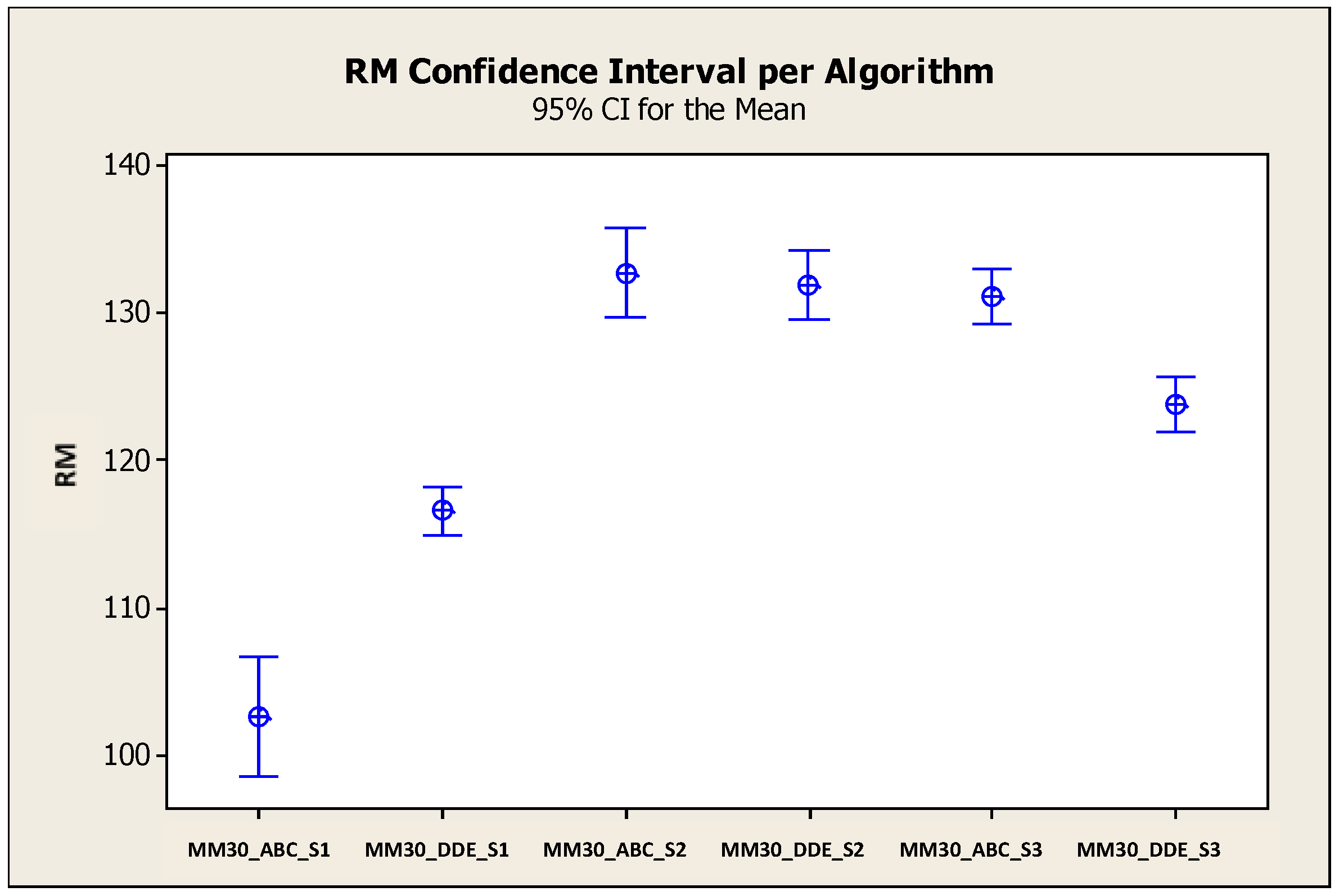
Stage	Measure	MM30		MM50		MM100
		ABC	DDE	ABC	DDE	ABC	DDE
S1	Avg. Dev.	0.00176	0.00580	0.04571	0.03104	0.04424	0.04031
	Std. Dev.	0.00664	0.01952	0.03946	0.06002	0.03257	0.04090
	Avg. RM.	102.75556	116.62593	116.62593	117.31481	117.39630	115.85185
S2	Avg. Dev.	0.09690	0.09524	0.10132	0.09640	0.08497	0.07570
	Std. Dev.	0.05793	0.08394	0.05917	0.08180	0.04307	0.05348
	Avg. RM.	132.72593	131.86296	133.81481	136.22593	137.12963	134.46670
S3	Avg. Dev.	0.05041	0.02491	0.05387	0.03711	0.04373	0.04259
	Std. Dev.	0.04794	0.04856	0.05220	0.05615	0.04067	0.04371
	Avg. RM.	100.62593	123.80370	124.45926	125.99259	127.43704	124.52593

presents the results obtained from evaluating all 270 instances of every benchmark set. The target, entropy-based, and resilient schedules in Stage I, II, and III are referred to as S1, S2, and S3, respectively. They were assessed based on two measures: the makespan (Avg. Dev.) and the robustness (Avg. RM.). Avg. Dev. refers to the average of all the deviations computed by (M_s − BKO)/BKO. M_s denotes the schedule makespan at the current stage, whereas the best-known makespan (BKO) represents the reference makespan, i.e., the optimal solution when comparing the target schedule of Stage I and the upper-bound schedule of Stage III. Furthermore, Avg. RM. is a measure of average robustness. Finally, the algorithmic performance was evaluated for three benchmark sets (i.e., MM30, MM50, and MM100) against the ABC.

The three-stage procedure proved to be robust enough to produce results comparable to different optimization algorithms. These results are encouraging, given that practitioners can add anywhere between 8% to 15% of their original estimates as response time intervals (i.e., buffer times). Furthermore, both ABC and DDE algorithms performed better when considering that response time intervals used by practitioners rely primarily on intuition and experience. On the other hand, this three-stage procedure relies solely on information available to every project, including activity durations and precedence.

Meanwhile, Figure 3, Figure 4 and Figure 5 show the results of the average deviation of every benchmark instance when compared against the BKO for every stage, divided according to the optimization algorithm applied. In addition, Figure 6, Figure 7 and Figure 8 show the robustness measures obtained at each stage using the DDE and ABC algorithms on different sizes of benchmark instances, i.e., MM30, MM50, and MM100.

Compared to the previously obtained results (columns marked with ABC), the most significant difference observed for the obtained solutions is their stability. Though the standard deviation of both algorithms increases with complexity, this increase is lower and slower when using DDE. Furthermore, the methodology remains stable and yields schedules with robust makespans near the best-known optima. In summary, better implementations of optimization algorithms can further improve the performance of the proposed methodology.

5. Conclusions

Uncertainty greatly impacts the dynamic behavior of real-world environments. Adaptive capacity helps to improve preparedness in dynamic environments, and managers must respond effectively to changes in environmental conditions. Researchers and practitioners have sought to optimize schedules and quality in many studies, and improving schedules remains a pressing concern. In this paper, we tried to resolve the multi-mode resource-constrained project scheduling problem (MRCPSP/max), which is not a common domain for the DDE algorithm, and we specifically considered entropy, which helped to deal with uncertainty.

We focus on three main contributions in this paper. Initially, we explored the characterization of MRCPSP/max under uncertainty conditions and confirmed the need for managers to recognize and positively respond to disruptive events. Using entropy to determine disruptive events and response intervals in scheduling, we demonstrated this proposition. Then, we formulated the robustness attribute as a scheduling adaptability maximization problem and a three-stage schedule generation framework to enhance resilience by absorbing the impact of unexpected events, while rescheduling during execution. Our final contribution was a discrete framework for the differential evolution algorithm. In our application of DDE, the encoding of the DDE algorithm consisted of two vectors representing the task sequence and the execution modes for each activity. Several potential resource conflicts and priority constraints were considered in our design. The proposed DDE was evaluated by solving test instances of benchmark sets by comparing its performance to the best known optima (BKO) and the previous application based on the artificial bee colony (ABC) approach.

The findings indicated that, for all algorithms, the problem’s complexity influences the number of optima found and the average run time. Overall, a more effective algorithm is the DDE algorithm, as it offers more optimal solutions and a higher number of them. Additionally, we were able to determine when practitioners need to add response time intervals at certain range levels, such as 8% to 15% in this case, to benefit from schedule robustness. Finally, compared to the BKO for every stage, the stability of the solutions provided by the DDE demonstrated its algorithmic advantage in terms of resilience. Unfortunately, the more realistic the academic model is, the more difficult it is to solve the problem; the MRCPSP/max is simply one of the very difficult problems.

Nonetheless, the encouraging computational results may lead to future implications along other lines. First of all, it is interesting to study which features make instances of MRCPSP/max difficult or easy to solve. In this sense, future studies may further enhance scheduling efficiency by examining various criteria for activity prioritization and mode selection. Another interesting line of research is investigating other potential encoding scheme frameworks in order to capture problem-specific aspects. Furthermore, efforts to examine other approaches to dealing with uncertainty in project scheduling and the verification of their performance using real-world data are also necessary.

References

- Alipouri, Y.; Sebt, M.H.; Ardeshir, A.; Chan, W.T. Solving the FS-RCPSP with hyper-heuristics: A policy-driven approach. J. Oper. Res. Soc. 2019, 70, 403–419. [Google Scholar] [CrossRef]
- Khodakarami, V.; Fenton, N.; Neil, M. Project Scheduling: Improved approach to incorporate uncertainty using Bayesian Networks. Proj. Manag. J. 2007, 38, 39–49. [Google Scholar] [CrossRef]
- Rezakhani, P. Project scheduling and performance prediction: A fuzzy-Bayesian network approach. In Engineering, Construction and Architectural Management; Emerald Publishing Limited Publisher: Bingley, UK, 2021. [Google Scholar]
- Ballestín, F. When it is worthwhile to work with the stochastic RCPSP? J. Sched. 2007, 10, 153–166. [Google Scholar] [CrossRef]
- Klerides, E.; Hadjiconstantinou, E. A decomposition-based stochastic programming approach for the project scheduling problem under time/cost trade-off settings and uncertain durations. Comput. Oper. Res. 2010, 37, 2131–2140. [Google Scholar] [CrossRef]
- Mokhtari, H.; Aghaie, A.; Rahimi, J.; Mozdgir, A. Project time–cost trade-off scheduling: A hybrid optimization approach. Int. J. Adv. Manuf. Technol. 2010, 50, 811–822. [Google Scholar] [CrossRef]
- Lambrechts, O.; Demeulemeester, E.; Herroelen, W. Time slack-based techniques for robust project scheduling subject to resource uncertainty. Ann. Oper. Res. 2011, 186, 443–464. [Google Scholar] [CrossRef]
- Moradi, H.; Shadrokh, S. A robust scheduling for the multimode project scheduling problem with a given deadline under uncertainty of activity duration. Int. J. Prod. Res. 2019, 57, 3138–3167. [Google Scholar] [CrossRef]
- Xiong, J.; Chen, Y.; Zhou, Z. Resilience analysis for project scheduling with renewable resource constraints and uncertain activity durations. J. Ind. Manag. Optim. 2016, 12, 719. [Google Scholar]
- Milat, M.; Knezic, S.; Sedlar, J. A new surrogate measure for a resilient approach to construction scheduling. Procedia Comput. Sci. 2021, 181, 468–476. [Google Scholar] [CrossRef]
- Askarifard, M.; Abbasianjahromi, H.; Sepehri, M.; Zeighami, E. A robust multi-objective optimization model for project scheduling considering risk and sustainable development criteria. Environ. Dev. Sustain. 2021, 23, 11494–11524. [Google Scholar] [CrossRef]
- Rahman, M.H.F.; Chakrabortty, R.K.; Ryan, M.J. Managing Uncertainty and Disruptions in Resource-Constrained Project Scheduling Problems: A Real-Time Reactive Approach. IEEE Access 2021, 9, 45562–45586. [Google Scholar] [CrossRef]
- Van de Vonder, S.; Demeulemeester, E.; Herroelen, W.; Leus, R. The use of buffers in project management: The trade-off between stability and makespan. Int. J. Prod. Econ. 2005, 97, 227–240. [Google Scholar] [CrossRef] [Green Version]
- Golab, A.; Gooya, E.; Falou, A.; Cabon, M. Review of conventional metaheuristic techniques for resource-constrained project scheduling problem. J. Proj. Manag. 2022, 7, 95–110. [Google Scholar] [CrossRef]
- Habibi, F.; Barzinpour, F.; Sadjadi, S. Resource-constrained project scheduling problem: Review of past and recent developments. J. Proj. Manag. 2018, 3, 55–88. [Google Scholar] [CrossRef]
- Hazır, Ö.; Ulusoy, G. A classification and review of approaches and methods for modeling uncertainty in projects. Int. J. Prod. Econ. 2020, 223, 107522. [Google Scholar] [CrossRef]
- Hartmann, S.; Briskorn, D. An Updated Survey of Variants and Extensions of the Resource-Constrained Project Scheduling Problem. Eur. J. Oper. Res. 2022, 297, 1–14. [Google Scholar] [CrossRef]
- Nansheng, P.; Qichen, M. Resource allocation in robust scheduling. J. Oper. Res. Soc. 2022, 1–18. [Google Scholar] [CrossRef]
- Bruni, M.E.; Pugliese, L.D.P.; Beraldi, P.; Guerriero, F. An adjustable robust optimization model for the resource-constrained project scheduling problem with uncertain activity durations. Omega 2017, 71, 66–84. [Google Scholar] [CrossRef]
- Bold, M.; Goerigk, M. A compact reformulation of the two-stage robust resource-constrained project scheduling problem. Comput. Oper. Res. 2021, 130, 105232. [Google Scholar] [CrossRef]
- Wang, Z.; Ng, T.S.; Pang, C.K. Minimizing activity exposures in project scheduling under uncertainty. Expert Syst. Appl. 2021, 173, 114635. [Google Scholar] [CrossRef]
- Kreter, S.; Schutt, A.; Stuckey, P.J.; Zimmermann, J. Mixed-integer linear programming and constraint programming formulations for solving resource availability cost problems. Eur. J. Oper. Res. 2018, 266, 472–486. [Google Scholar] [CrossRef]
- Li, H.; Xiong, L.; Liu, Y.; Li, H. An effective genetic algorithm for the resource levelling problem with generalised precedence relations. Int. J. Prod. Res. 2018, 56, 2054–2075. [Google Scholar] [CrossRef]
- Mahalleh, M.K.K.; Ashjari, B.; Yousefi, F.; Saberi, M. A robust solution to resource-constraint project scheduling problem. Int. J. Fuzzy Log. Intell. Syst. 2017, 17, 221–227. [Google Scholar] [CrossRef] [Green Version]
- Davari, M.; Demeulemeester, E. The proactive and reactive resource-constrained project scheduling problem. J. Sched. 2019, 22, 211–237. [Google Scholar] [CrossRef]
- Chen, A.H.L.; Liang, Y.C.; Padilla, J.D. An entropy-based upper bound methodology for robust predictive multimode RCPSP schedules. Entropy 2014, 16, 5032–5067. [Google Scholar] [CrossRef] [Green Version]
- Chen, A.H.L.; Liang, Y.C.; Padilla, J.D. Using discrete differential evolution and Entropy to solve the MRCPSP. In Proceedings of the 2017 IEEE Congress on Evolutionary Computation (CEC), Donostia, Spain, 5–8 June 2017; pp. 2437–2442. [Google Scholar]
- Elmaghraby, S.E. Activity Networks: Project Planning and Control by Network Models; John Wiley & Sons: Hoboken, NJ, USA, 1977. [Google Scholar]
- Bartusch, M.; Möhring, R.H.; Radermacher, F.J. Scheduling project networks with resource constraints and time windows. Ann. Oper. Res. 1988, 16, 199–240. [Google Scholar] [CrossRef]
- Bushuyev, S.D.; Sochnev, S.V. Entropy measurement as a project control tool. Int. J. Proj. Manag. 1999, 17, 343–350. [Google Scholar] [CrossRef]
- Asllani, A.; Ettkin, L. An entropy-based approach for measuring project uncertainty. Acad. Inf. Manag. Sci. J. 2007, 10, 31–45. [Google Scholar]
- Song, H.; Wu, D.; Li, M.; Cai, C.; Li, J. An entropy based approach for software risk assessment: A perspective of trustworthiness enhancement. In Proceedings of the 2nd International Conference on Software Engineering and Data Mining, Chengdu, China, 23–25 June 2010; pp. 575–578. [Google Scholar]
- Tseng, C.C.; Ko, P.W. Measuring schedule uncertainty for a stochastic resource-constrained project using scenario-based approach with utility-entropy decision model. J. Ind. Prod. Eng. 2016, 33, 558–567. [Google Scholar] [CrossRef]
- Chenarani, A.; Druzhinin, E.A. A quantitative measure for evaluating project uncertainty under variation and risk effects. Eng. Technol. Appl. Sci. Res. 2017, 7, 2083–2088. [Google Scholar] [CrossRef]
- Christodoulou, S.E. Entropy-based heuristic for resource-constrained project scheduling. J. Comput. Civ. Eng. 2017, 31, 04016068. [Google Scholar] [CrossRef]
- Qiao, J.; Li, Y. Resource leveling using normalized Entropy and relative Entropy. Autom. Constr. 2018, 87, 263–272. [Google Scholar] [CrossRef]
- Vanhoucke, M.; Batselier, J. A statistical method for estimating activity uncertainty parameters to improve project forecasting. Entropy 2019, 21, 952. [Google Scholar] [CrossRef] [Green Version]
- Shannon, C.E. A mathematical theory of communication. Bell Syst. Tech. J. 1948, 27, 379–423. [Google Scholar] [CrossRef] [Green Version]
- Norris, F.H.; Stevens, S.P.; Pfefferbaum, B.; Wyche, K.F.; Pfefferbaum, R.L. Community resilience as a metaphor, theory, set of capacities, and strategy for disaster readiness. Am. J. Community Psychol. 2008, 41, 127–150. [Google Scholar] [CrossRef]
- Al-Fawzan, M.A.; Haouari, M. A bi-objective model for robust resource-constrained project scheduling. Int. J. Prod. Econ. 2005, 96, 175–187. [Google Scholar] [CrossRef]
- Kobylański, P.; Kuchta, D. A note on the paper by MA Al-Fawzan and M. Haouari about a bi-objective problem for robust resource-constrained project scheduling. Int. J. Prod. Econ. 2007, 107, 496–501. [Google Scholar] [CrossRef]
- Ma, G.; Gu, L.; Li, N. Scenario-based proactive robust optimization for critical-chain project scheduling. J. Constr. Eng. Manag. 2015, 141, 04015030. [Google Scholar] [CrossRef]
- Balouka, N.; Cohen, I. A robust optimization approach for the multimode resource-constrained project scheduling problem. Eur. J. Oper. Res. 2019, 291, 457–470. [Google Scholar] [CrossRef]
- Burgelman, J.; Vanhoucke, M. Project schedule performance under general mode implementation disruptions. Eur. J. Oper. Res. 2020, 280, 295–311. [Google Scholar] [CrossRef]
- Chtourou, H.; Haouari, M. A two-stage-priority-rule-based algorithm for robust resource-constrained project scheduling. Comput. Ind. Eng. 2008, 55, 183–194. [Google Scholar] [CrossRef]
- Talbot, F.B. Resource-constrained project scheduling with time-resource tradeoffs: The non-preemptive case. Manag. Sci. 1982, 28, 1197–1210. [Google Scholar] [CrossRef]
- Chen, A.H.L.; Liang, Y.C.; Padilla, J.D. A practical and robust execution time-frame procedure for the multi-mode resource-constrained project scheduling problem with minimal and maximal time lags. Algorithms 2016, 9, 63. [Google Scholar] [CrossRef] [Green Version]
- Storn, R.; Price, K. Differential evolution–a simple and efficient heuristic for global optimization over continuous spaces. J. Glob. Optim. 1997, 11, 341–359. [Google Scholar] [CrossRef]
- Mohapatra, P.; Roy, S.; Das, K.N.; Dutta, S.; Raju, M.S.S. A review of evolutionary algorithms in solving large scale benchmark optimisation problems. Int. J. Math. Oper. Res. 2022, 21, 104–126. [Google Scholar] [CrossRef]
- Pant, M.; Zaheer, H.; Garcia-Hernandez, L.; Abraham, A. Differential Evolution: A review of more than two decades of research. Eng. Appl. Artif. Intell. 2020, 90, 103479. [Google Scholar]
- Han, Y.; Li, J.; Sang, H.; Liu, Y.; Gao, K.; Pan, Q. Discrete evolutionary multi-objective optimization for energy-efficient blocking flow shop scheduling with setup time. Appl. Soft Comput. 2020, 93, 106343. [Google Scholar] [CrossRef]
- de Fátima Morais, M.; Ribeiro, M.H.D.M.; da Silva, R.G.; Mariani, V.C.; dos Santos Coelho, L. Discrete differential evolution metaheuristics for permutation flow shop scheduling problems. Comput. Ind. Eng. 2022, 166, 107956. [Google Scholar] [CrossRef]
- Öztop, H.; Tasgetiren, M.F.; Kandiller, L.; Pan, Q.K. Metaheuristics with restart and learning mechanisms for the no-idle flowshop scheduling problem with makespan criterion. Comput. Oper. Res. 2022, 138, 105616. [Google Scholar] [CrossRef]
- Yuan, Y.; Xu, H. Flexible job shop scheduling using hybrid differential evolution algorithms. Comput. Ind. Eng. 2013, 65, 246–260. [Google Scholar] [CrossRef]
- Zhao, F.; Shao, Z.; Wang, J.; Zhang, C. A hybrid differential evolution and estimation of distribution algorithm based on neighbourhood search for job shop scheduling problems. Int. J. Prod. Res. 2016, 54, 1039–1060. [Google Scholar] [CrossRef]
- Zhang, G.; Xing, K.; Cao, F. Discrete differential evolution algorithm for distributed blocking flow shop scheduling with makespan criterion. Eng. Appl. Artif. Intell. 2018, 76, 96–107. [Google Scholar] [CrossRef]
- Wu, X.; Liu, X.; Zhao, N. An improved differential evolution algorithm for solving a distributed assembly flexible job shop scheduling problem. Memetic Comput. 2019, 11, 335–355. [Google Scholar] [CrossRef]
- Ali, I.M.; Essam, D.; Kasmarik, K. A novel design of differential evolution for solving discrete traveling salesman problems. Swarm Evol. Comput. 2020, 52, 100607. [Google Scholar] [CrossRef]
- Zhao, F.; Zhao, L.; Wang, L.; Song, H. An ensemble discrete differential evolution for the distributed blocking flow shop scheduling with minimizing makespan criterion. Expert Syst. Appl. 2020, 160, 113678. [Google Scholar] [CrossRef]
- Yuan, S.; Li, T.; Wang, B. A discrete differential evolution algorithm for flow shop group scheduling problem with sequence-dependent setup and transportation times. J. Intell. Manuf. 2021, 32, 427–439. [Google Scholar] [CrossRef]
- Moraglio, A.; Togelius, J.; Silva, S. Geometric differential evolution for combinatorial and programs spaces. Evol. Comput. 2013, 21, 591–624. [Google Scholar] [CrossRef] [PubMed] [Green Version]
- Krömer, P.; Uher, V.; Snášel, V. Novel Random Key Encoding Schemes for the Differential Evolution of Permutation Problems. IEEE Trans. Evol. Comput. 2022, 26, 43–57. [Google Scholar] [CrossRef]
- Liu, Y.; Chen, W.N.; Zhan, Z.H.; Lin, Y.; Gong, Y.J.; Zhang, J. A set-based discrete differential evolution algorithm. In Proceedings of the 2013 IEEE International Conference on Systems, Man, and Cybernetics, Manchester, UK, 13–16 October 2013; pp. 1347–1352. [Google Scholar]
- Baioletti, M.; Milani, A.; Santucci, V. Variable neighborhood algebraic differential evolution: An application to the linear ordering problem with cumulative costs. Inf. Sci. 2020, 507, 37–52. [Google Scholar] [CrossRef]
- Santucci, V.; Baioletti, M.; Di Bari, G. An improved memetic algebraic differential evolution for solving the multidimensional two-way number partitioning problem. Expert Syst. Appl. 2021, 178, 114938. [Google Scholar] [CrossRef]
- Wang, L.; Fu, X.; Mao, Y.; Menhas, M.I.; Fei, M. A novel modified binary differential evolution algorithm and its applications. Neurocomputing 2012, 98, 55–75. [Google Scholar] [CrossRef]
- Pampara, G.; Engelbrecht, A.P.; Franken, N. Binary differential evolution. In Proceedings of the 2006 IEEE International Conference on Evolutionary Computation, Vancouver, BC, Canada, 16–21 July 2006; pp. 1873–1879. [Google Scholar]
- Damak, N.; Jarboui, B.; Siarry, P.; Loukil, T. Differential evolution for solving multimode resource-constrained project scheduling problems. Comput. Oper. Res. 2009, 36, 2653–2659. [Google Scholar] [CrossRef]
- Kazemipoor, H.; Tavakkoli-Moghaddam, R.; Shahnazari-Shahrezaei, P.; Azaron, A. A differential evolution algorithm to solve multi-skilled project portfolio scheduling problems. Int. J. Adv. Manuf. Technol. 2013, 64, 1099–1111. [Google Scholar] [CrossRef]
- Peng, W.; Huang, M. A critical chain project scheduling method based on a differential evolution algorithm. Int. J. Prod. Res. 2014, 52, 3940–3949. [Google Scholar] [CrossRef]
- Zhang, L.; Luo, Y.; Zhang, Y. Hybrid particle swarm and differential evolution algorithm for solving multimode resource-constrained project scheduling problem. J. Control Sci. Eng. 2015, 2015, 48. [Google Scholar] [CrossRef] [Green Version]
- Eshraghi, A. A new approach for solving resource constrained project scheduling problems using differential evolution algorithm. Int. J. Ind. Eng. Comput. 2016, 7, 205–216. [Google Scholar] [CrossRef]
- Sallam, K.M.; Chakrabortty, R.K.; Ryan, M.J. A hybrid differential evolution with cuckoo search for solving resource-constrained project scheduling problems. In Proceedings of the 2019 IEEE International Conference on Industrial Engineering and Engineering Management (IEEM), Macao, China, 15–18 December 2019; pp. 1344–1348. [Google Scholar]
- Quoc, H.D.; The, L.N.; Doan, C.N.; Thanh, T.P. New Effective Differential Evolution Algorithm for the Project Scheduling Problem. In Proceedings of the 2020 2nd International Conference on Computer Communication and the Internet (ICCCI), Nagoya, Japan, 26–29 June 2020; pp. 150–157. [Google Scholar]
- Institute of Management and Economics, TU Clausthal. Multi Mode Project Duration Problem MRCPSP/Max. Available online: https://www.wiwi.tu-clausthal.de/en/ueber-uns/abteilungen/betriebswirtschaftslehre-insbesondere-produktion-und-logistik/research/research-areas/project-generator-progen/max-and-psp/max-library/multi-mode-project-duration-problem-mrcpsp/max (accessed on 7 October 2020).