Dynamic Response of Slope Inertia-Based Timoshenko Beam under a Moving Load

Abstract

In this paper, the dynamic response of a simply supported beam subjected to a moving load is reinvestigated. Based on a new beam theory, slope inertia-based Timoshenko (SIBT), the governing equations of motion of the beam are derived. An analytical solution is presented by using a coupled Fourier and Laplace–Carson integral transformation method. The finite element solution is also developed and compared with the analytical solution. Then, a comparative study of three beam models based on the SIBT, Euler–Bernoulli and Timoshenko, subjected to a moving load, is presented. The results show that for slender beams, the dynamic responses calculated by the three theories have marginal differences. However, as the ratio of the cross-sectional size to beam length increases, the dynamic magnification factors for the mid-span displacement obtained by the SIBT and Timoshenko beams become larger than those obtained by the Euler–Bernoulli beams. Furthermore, until the ratio is greater than 1/3, the difference between the calculated results of the SIBT and Timoshenko beams becomes apparent.

1. Introduction

The analysis of moving loads on engineering structures has been a major research topic since the mid-19th century [1]. To its credit is the excellent monograph by Fryba [2], which describes many classical moving load problems and their analytical solution. Motivated by the increasing high-speed rail lines, the vibration and control of beams, especially under moving loads, naturally arouses the renewed interest of researchers and engineers [3,4,5,6].

So far, the Euler–Bernoulli beam theory is still the most commonly used in the dynamic analysis of engineering structures, owing to its simplicity and reasonable engineering approximations. Based on this theory, many analytical and numerical methods have been developed to address the moving load problems [7,8,9,10,11]. Although the Euler–Bernoulli model has been proven to be accurate enough for slender beams, it tends to overestimate the natural frequencies of deep beams and their higher vibrational modes [4,12].

Another famous beam theory, the Timoshenko beam theory [13,14,15], which takes into account both the shear deformation and rotary inertia of the cross section, is also widely used. Many analytical and numerical methods have also been developed to address the moving loads problems, for example [16,17,18,19]. Despite substantial research and applications on the Timoshenko model having been carried out over 100 years, there are still open questions deserving further discussion [12,20,21]. The most controversial point about this model is the second frequency spectrum [4,22]. Nesterenko [23] and Stehen [24] indicated that the second frequency spectrum is physically meaningless and should be disregarded. In contrast, Cazzani et al. [25,26] and Diaz-de-Anda et al. [27] opined that the second frequency spectrum is valuable and should be retained.

Several researchers suggested dropping off the fourth-order time derivative term in the equation of motion of the Timoshenko model since the deformation caused by this term is negligible [28] and the physical meaning of the term itself is not clear [4]. For example, Chen et al. [29] and Elishakoff et al. [15] respectively considered the rotary inertia caused by shear deformation and proposed the truncated Timoshenko beam theory (TTBT). However, further studies have shown that the TTBT is asymptotically consistent, for it cannot be variationally derived [22].

Recently, Elishakoff et al. [22,30,31,32] proposed a slope inertia-based Timoshenko (SIBT) beam theory by means of the variational approach. Using the deflection slope instead of the bending rotation in the kinetic energy expression, the SIBT model eliminates the fourth-order time derivative term associated with the Timoshenko model and appears to be preferable to the TTBT [22]. Xia et al. [4] carried out analytical and numerical studies on the SIBT model to clarify the physical meaning of its governing equation terms and reveal its distinct features in the prediction of modes and frequencies. Although the SIBT seems to be more comprehensive and preferable, a fundamental study of the SIBT beam under a moving load problem is not available yet.

In this paper, based on the SIBT theory, the governing equations of motion of the beam under a moving load are established. An analytical solution to this problem is presented. Next, the finite element solution is proposed and validated. We present a comparative study of the SIBT, Euler–Bernoulli and Timoshenko beam models subjected to a moving load. Finally, concluding remarks are given.

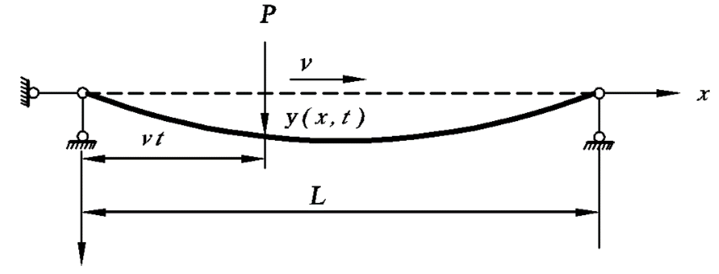
2. Problem Definition

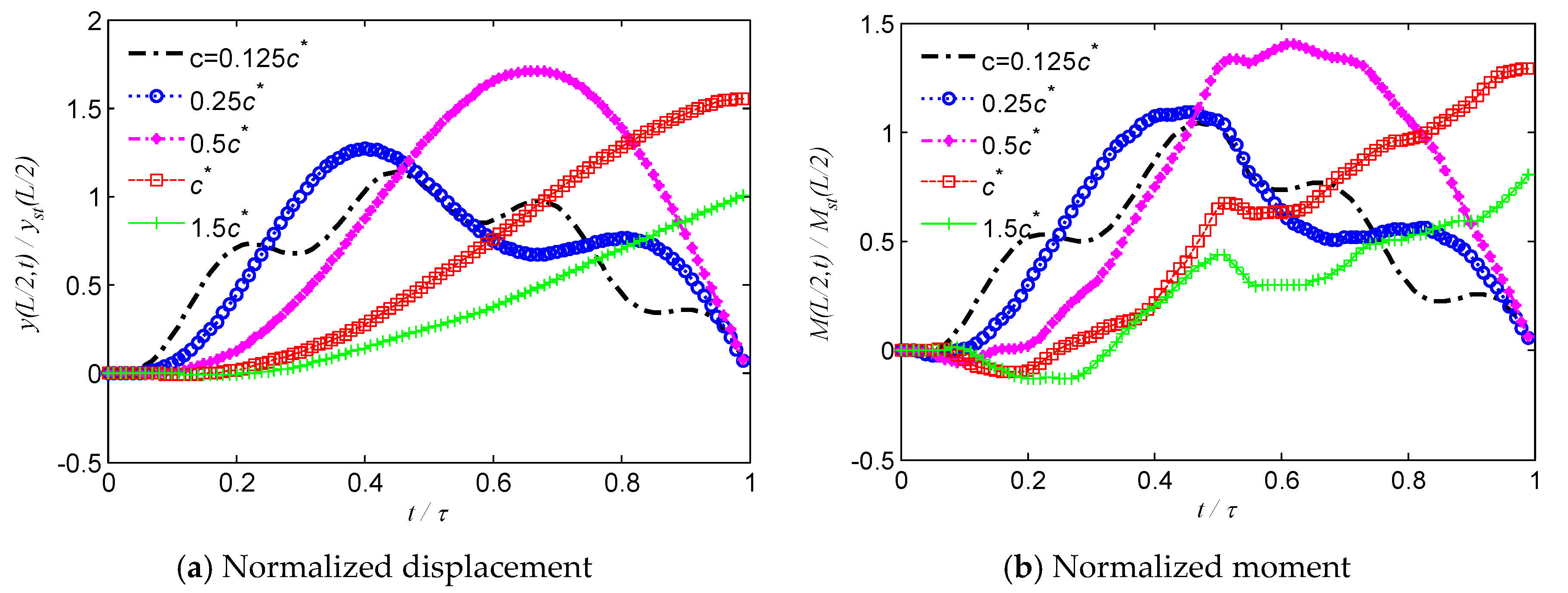
Consider a simply supported beam traversed by a moving concentrated load P as shown in Figure 1. The Hamilton’s principle is employed to establish the equations of forced vibration of the beam by extending the SIBT equations for free vibration [4,22]. The kinetic energy T of the beam, the strain energy U, and the work done W due to the moving load P can be written as

$$T=\frac{1}{2}{\displaystyle \underset{0}{\overset{L}{\int }}\rho A{\left(\frac{\partial y}{\partial t}\right)}^2}dx+\frac{1}{2}{\displaystyle \underset{0}{\overset{L}{\int }}\rho I{\left(\frac{{\partial }^{2}y}{\partial t\partial x}\right)}^2}dx$$

(1)

$$U=\frac{1}{2}{\displaystyle \underset{0}{\overset{L}{\int }}EI{\left(\frac{\partial \phi }{\partial x}\right)}^2}dx+\frac{1}{2}{\displaystyle \underset{0}{\overset{L}{\int }}kGA{\left(\frac{\partial y}{\partial x}-\phi \right)}^2}dx$$

(2)

$$W={\displaystyle \underset{0}{\overset{L}{\int }}\delta (x-vt)Py}dx$$

(3)

where the vertical displacement of the beam is y (x, t) for $0\le x\le L$ and $0\le t\le \tau$, where $\tau =L/v$ is the traversing time of the load P on the beam. $\phi$ is the bending rotation of the beam, and $\delta$ is the Dirac delta function. Instead of pure bending rotary inertia in the Timoshenko model, $\rho I{(\partial \phi /\partial t)}^2$, the slope inertia, $\rho I{({\partial }^{2}y/\partial x\partial t)}^2$, is used to incorporate the shear inertia in the kinetic energy (see Equation (1)). By applying Hamilton’s principle, we obtain the two coupled differential equations of motion of the beam subjected to a moving load as

$$\rho A\frac{{\partial }^{2}y}{\partial t^2}-kGA\left(\frac{{\partial }^{2}y}{\partial x^2}-\frac{\partial \phi }{\partial x}\right)-\rho I\frac{{\partial }^{4}y}{\partial x^2\partial t^2}=\delta (x-vt)P$$

(4)

$$EI\frac{{\partial }^2\phi }{\partial x^2}+kGA\left(\frac{\partial y}{\partial x}-\phi \right)=0$$

(5)

The boundary conditions are given by Equation (6)

$$\left(EI\frac{\partial \phi }{\partial x}\right)\delta \phi |{}_0^L=0,\begin{array}{cc}& \left[kGA\left(\frac{\partial y}{\partial x}-\phi \right)+\rho I\left(\frac{{\partial }^{3}y}{\partial t^2\partial x}\right)\right]\end{array}\delta y|{}_0^L=0$$

(6)

where $\delta y$ and $\delta \phi$ represent the variation of displacement and bending rotation of the beam, respectively. To satisfy these conditions, for a simply supported beam, the boundary and the initial conditions are given as

$$y(0,t)=0,\begin{array}{cc}& \frac{\partial \phi }{\partial x}(0,t)=0,\begin{array}{cc}& y(L,t)=0,\begin{array}{cc}& \frac{\partial \phi }{\partial x}(L,t)=0\end{array}\end{array}\end{array}$$

(7)

$$y(x,0)=0,\begin{array}{cc}& \frac{\partial y}{\partial t}(x,0)=0,\begin{array}{cc}& \phi (x,0)=0,\begin{array}{cc}& \frac{\partial \phi }{\partial t}(x,0)=0\end{array}\end{array}\end{array}$$

(8)

3. Results

To solve the problem analytically, we apply a coupled finite integral transformation method. Firstly, for the transverse displacement y, one may employ the Fourier sine transformation. For the bending rotation $\phi$, the Fourier cosine transformation is used.

$$Y(j,t)={\displaystyle \underset{0}{\overset{L}{\int }}y(x,t)\sin \frac{j\pi x}{L}}dx,\begin{array}{cc}& j=1,2,3,\dots \end{array}$$

(9)

$$y(x,t)=\frac{2}{L}{\displaystyle \sum _{j=1}^{\infty }Y(j,t)\sin \frac{j\pi x}{L}}$$

(10)

$$\psi (j,t)={\displaystyle \underset{0}{\overset{L}{\int }}\phi (x,t)\cos \frac{j\pi x}{L}}dx,\begin{array}{cc}& j=1,2,3,\dots \end{array}$$

(11)

$$\phi (x,t)=\frac{2}{L}{\displaystyle \sum _{j=1}^{\infty }\psi (j,t)\cos \frac{j\pi x}{L}}$$

(12)

where $Y(j,t)$ and $\psi (j,t)$ are image functions of $y(x,t)$ and $\phi (x,t)$, respectively. Multiply Equations (4) and (5) with $\sin \frac{j\pi x}{L}$ and $\cos \frac{j\pi x}{L}$, respectively, and integrate them with respect to x over a finite interval $\left[0,L\right]$. The following is obtained considering the boundary conditions stated in Equation (7):

$$\rho A\ddot{Y}(j,t)-kGA\left(-\frac{j^2{\pi }^2}{L^2}Y(j,t)+\frac{j\pi }{L}\psi (j,t)\right)+\rho I\frac{j^2{\pi }^2}{L^2}\ddot{Y}(j,t)=P\sin \frac{j\pi vt}{L}$$

(13)

$$-EI\frac{j^2{\pi }^2}{L^2}\psi (j,t)+kGA\left(\frac{j\pi }{L}Y(j,t)-\psi (j,t)\right)=0$$

(14)

Substituting Equation (14) into Equation (13), one obtains

$$\left(\rho A+\rho I{j}^2{\pi }^2/L^2\right)\ddot{Y}(j,t)+\frac{EIkGA{j}^4{\pi }^4/L^4}{kGA+EI{j}^2{\pi }^2/L^2}Y(j,t)=P\sin \frac{j\pi vt}{L}$$

(15)

which can be rewritten as

$$\ddot{Y}(j,t)+{\omega }_j^{2}Y(j,t)=P_j\sin {\overline{\omega }}_{j}t$$

(16)

where

$${\omega }_j^2=\frac{EIkGA{j}^4{\pi }^4/L^4}{\left(kGA+EI{j}^2{\pi }^2/L^2\right)\left(\rho A+\rho I{j}^2{\pi }^2/L^2\right)}$$

(17)

$$P_j=\frac{P}{\left(\rho A+\rho I{j}^2{\pi }^2/L^2\right)}$$

(18)

$${\overline{\omega }}_j=j\pi v/L$$

(19)

Equation (16) depicts a harmonic vibration without damping and can be solved according to Chopra [32]. Herein, the Laplace–Carson transformation method [2] is applied, which leads to

$$Y^{*}(j,s)=s{\displaystyle \underset{0}{\overset{\infty }{\int }}Y(j,t)e^{-st}dt}$$

(20)

Transforming Equation (16) in accordance with Equation (20), and in view of the initial condition as Equation (8), one obtains

$$s^2{Y}^{*}(j,s)+{\omega }_j^2{Y}^{*}(j,s)=P_j{\overline{\omega }}_j\frac{s}{s^2+{\overline{\omega }}_j^2}$$

(21)

By rearrangement, Equation (21) can be written as

$$Y^{*}(j,s)=P_j{\overline{\omega }}_j\frac{s}{s^2+{\overline{\omega }}_j^2}\frac{1}{s^2+{\omega }_j^2}$$

(22)

According to the inverse Laplace–Carson transformation [2], the image function $Y(j,t)$ can be obtained as

$$Y(j,t)=\frac{P_j}{{\omega }_j^2(1-{\beta }_j^2)}\left(\sin {\overline{\omega }}_{j}t-{\beta }_j\sin {\omega }_{j}t\right)\begin{array}{cc}& \begin{array}{cc}& \end{array}{\beta }_j\ne 1\end{array}$$

(23)

$$Y(j,t)=\frac{P_j}{2{\omega }_j^2}\left(\sin {\omega }_{j}t-{\omega }_{j}t\cos {\omega }_{j}t\right)\begin{array}{cc}& \begin{array}{cc}& \end{array}{\beta }_j=1\end{array}$$

(24)

where ${\beta }_j$ is the frequency ratio, defined as

$${\beta }_j={\overline{\omega }}_j/{\omega }_j$$

(25)

Substituting Equations (23) and (24) into Equation (14), $\psi (j,t)$ can be expressed as

$$\psi (j,t)=\frac{P_j}{{\omega }_j^2(1-{\beta }_j^2)}\left(\sin {\overline{\omega }}_{j}t-{\beta }_j\sin {\omega }_{j}t\right)kGA\left(\frac{j\pi }{L}\right)/\left(EI\frac{j^2{\pi }^2}{L^2}+kGA\right)\begin{array}{cc}& {\beta }_j\ne 1\end{array}$$

(26)

$$\psi (j,t)=\frac{P_j}{2{\omega }_j^2}\left(\sin {\omega }_{j}t-{\omega }_{j}t\cos {\omega }_{j}t\right)kGA\left(\frac{j\pi }{L}\right)/\left(EI\frac{j^2{\pi }^2}{L^2}+kGA\right)\begin{array}{cc}& {\beta }_j=1\end{array}$$

(27)

At last, substituting Equations (23), (24), (26) and (27) into Equations (10) and (12), one obtains the series solutions of the original functions $y(x,t)$ and $\phi (x,t)$

$$\begin{array}{ll}y(x,t)& =\frac{2}{L}{\displaystyle \sum _{\begin{array}{l}j=1\\ j\ne \alpha \end{array}}^{\infty }\frac{P_j{j}^2}{{\omega }_j^2(j^2-{\alpha }^2)}\left(\sin {\overline{\omega }}_{j}t-\frac{\alpha }{j}\sin {\omega }_{j}t\right)\sin \frac{j\pi x}{L}}\\ & +\frac{P_{\alpha }}{{\omega }_{\alpha }^{2}L}\left(\sin {\omega }_{\alpha }t-{\omega }_{\alpha }t\cos {\omega }_{\alpha }t\right)\sin \frac{\alpha \pi x}{L}\end{array}$$

(28)

$$\begin{array}{ll}\phi (x,t)& =\frac{2}{L}{\displaystyle \sum _{\begin{array}{l}j=1\\ j\ne \alpha \end{array}}^{\infty }\frac{P_j{j}^2}{{\omega }_j^2(j^2-{\alpha }^2)}\left(\sin {\overline{\omega }}_{j}t-\frac{\alpha }{j}\sin {\omega }_{j}t\right)\cos \frac{j\pi x}{L}}kGA\left(\frac{j\pi }{L}\right)/\left(EI\frac{j^2{\pi }^2}{L^2}+kGA\right)\\ & +\frac{P_{\alpha }}{{\omega }_{\alpha }^{2}L}\left(\sin {\omega }_{\alpha }t-{\omega }_{\alpha }t\cos {\omega }_{\alpha }t\right)\cos \frac{\alpha \pi x}{L}kGA\left(\frac{\alpha \pi }{L}\right)/\left(EI\frac{{\alpha }^2{\pi }^2}{L^2}+kGA\right)\end{array}$$

(29)

where the non-dimensional parameter $\alpha$ is defined by Equation (30) as

$$\alpha =j{\beta }_j$$

(30)

Equations (28) and (29) represent the transverse displacement and rotation solutions, respectively, for a simply supported beam subjected to a moving concentrated load. The bending moment $M(x,t)$ and shear force $Q(x,t)$ of the beam can be easily obtained as Equations (31) and (32).

$$M(x,t)=-EI\frac{\partial \phi (x,t)}{\partial x}$$

(31)

$$Q(x,t)=kGA\left(\frac{\partial y(x,t)}{\partial x}-\phi (x,t)\right)+\rho I\left(\frac{{\partial }^{3}y(x,t)}{\partial t^2\partial x}\right)$$

(32)

The analytical method is employed to investigate a beam with a circular cross section [17,33,34,35] subjected to a moving load (see Figure 1). The beam parameters and material properties are given in

Table 1. Parameters and properties of the beam.

Parameters	Value
Beam length L	1 m
Young’s modulus E	2.07 × 1011 N/m2
Shear modulus G	7.76 × 1010 N/m2
Shear correction coefficient $k$	0.9
Density $\rho$	7700 kg/m3
Circular cross-sectional area A	$4\pi r_0^2$
Area moment of inertia I	$4\pi r_0^4$

. The radius of gyration $r_0$ can be defined by a given non-dimensional parameter $b=r_0\pi /L$. The magnitude of the load is $P=0.2\rho ALg$. The speed of the moving load $v$, is defined as $v=c{v}_{cr}$, where $c$ is a non-dimensional parameter, and $v_{cr}$ is the critical speed given by $v_{cr}=\left(\pi /L\right)\sqrt{EI/\rho A}$, which is equal to ${\omega }_1^{*}L/\pi$, where ${\omega }_1^{*}$ is the fundamental frequency of a simply supported Euler–Bernoulli beam. The normalized displacement and bending moment of the beam are defined as $y(x,t)/y_{st}(L/2)$ and $M(x,t)/M_{st}(L/2)$, respectively. Note that $y_{st}(L/2)$ = $P{L}^3/48EI$ and $M_{st}(L/2)$ = $PL/4$ are the static mid-span displacement and the bending moment when the P located at mid-span for an Euler–Bernoulli beam, respectively.

The normalized mid-span displacement and bending moment of a beam with $b=0.03$ and $c=0.11$ for different truncated series solutions are given in Figure 2. The series solution of displacement converges very fast and may be truncated after the first 4 modes, but the convergence of the bending moment is slower, especially when the load moves close to the middle part of the beam. As can be seen from Figure 2b, at least 12 modes are required to achieve a satisfactory degree of accuracy.

4. Finite Element Solution

A finite element procedure is developed to analyze the same simply supported beam subjected to a moving load. The governing equations of motion are also derived according to Hamilton’s principle [36].

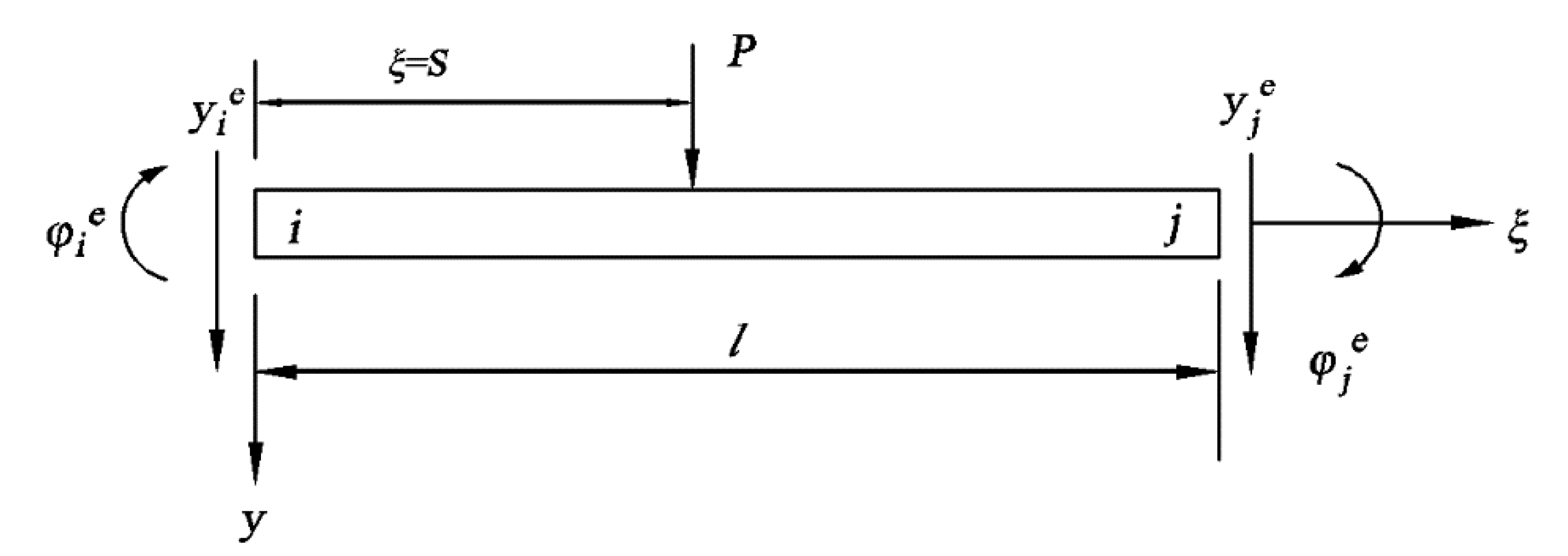
4.1. Shape Functions

The shape functions proposed by Reddy [37] are used to interpolate the nodal displacements and bending rotations of the beam elements. Figure 3 shows a typical SIBT beam element of length l traversed by a constant moving load. The displacement and bending rotation of an arbitrary location in the element can be expressed as

$$y=\left[\begin{array}{cccc}{N}_{y_1}& N_{y_2}& N_{y_3}& N_{y_4}\end{array}\right]\left\{\begin{array}{c}{y}_i^e\\ {\phi }_i^e\\ y_j^e\\ {\phi }_j^e\end{array}\right\}=\left[N_y\right]{\left\{q\right\}}^e$$

(33)

$$\phi =\left[\begin{array}{cccc}{N}_{{\phi }_1}& N_{{\phi }_2}& N_{{\phi }_3}& N_{{\phi }_4}\end{array}\right]\left\{\begin{array}{c}{y}_i^e\\ {\phi }_i^e\\ y_j^e\\ {\phi }_j^e\end{array}\right\}=\left[N_{\phi }\right]{\left\{q\right\}}^e$$

(34)

Herein, ${\left\{q\right\}}^e$ is the element nodal displacement vector, and $N_{yi}$, $N_{\phi i}$ (i = 1~4) are the shape functions.

4.2. Derivation of Element Matrices

The flexural strain or curvature $\chi$ and the shear strain $\gamma$ within the element can be expressed as

$$\chi =\frac{\partial \phi }{\partial x}=\left[B_b\right]{\left\{q\right\}}^e$$

(35)

$$\gamma =\frac{\partial y}{\partial x}-\phi =\left[B_s\right]{\left\{q\right\}}^e$$

(36)

where

$$\{\begin{array}{l}\left[B_b\right]=\frac{\partial }{\partial x}\left[N_{\phi }\right]\hfill \\ \left[B_s\right]=\frac{\partial }{\partial x}\left[N_y\right]-\left[N_{\phi }\right]=\left[B_y\right]-\left[N_{\phi }\right]\hfill \end{array}\{\begin{array}{l}\left[B_b\right]=\frac{\partial }{\partial x}\left[N_{\phi }\right]\hfill \\ \left[B_s\right]=\frac{\partial }{\partial x}\left[N_y\right]-\left[N_{\phi }\right]=\left[B_y\right]-\left[N_{\phi }\right]\hfill \end{array}$$

(37)

With the help of Equations (33)–(37), Equations (1)–(3) can be rewritten in terms of the element displacement vector ${\left\{q\right\}}^e$ as

$$T^e=\frac{1}{2}{\left\{\dot{q}\right\}}^{e,\mathrm{T}}{\left[M_t\right]}^e{\left\{\dot{q}\right\}}^e+\frac{1}{2}{\left\{\dot{q}\right\}}^{e,\mathrm{T}}{\left[M_r\right]}^e{\left\{\dot{q}\right\}}^e$$

(38)

$$U^e=\frac{1}{2}{\left\{q\right\}}^{e,\mathrm{T}}{\left[K_b\right]}^e{\left\{q\right\}}^e+\frac{1}{2}{\left\{q\right\}}^{e,\mathrm{T}}{\left[K_s\right]}^e{\left\{q\right\}}^e$$

(39)

$$W^e={\left\{F(t)\right\}}^e{\left\{q\right\}}^e$$

(40)

where the translational mass matrix ${\left[M_t\right]}^e$, slope mass matrix ${\left[M_r\right]}^e$, bending stiffness matrix ${\left[K_b\right]}^e$, shear stiffness matrix ${\left[K_s\right]}^e$, and equivalent nodal force vector ${\left\{F(t)\right\}}^e$ are written as

$$\{\begin{array}{l}{\left[M_t\right]}^e={{\displaystyle \underset{0}{\overset{l}{\int }}\left[N_y\right]}}^{\mathrm{T}}\rho A\left[N_y\right]d\xi \hfill \\ {\left[M_r\right]}^e={{\displaystyle \underset{0}{\overset{l}{\int }}\left[B_y\right]}}^{\mathrm{T}}\rho I\left[B_y\right]d\xi \hfill \\ {\left[K_b\right]}^e={{\displaystyle \underset{0}{\overset{l}{\int }}\left[B_b\right]}}^{\mathrm{T}}EI\left[B_b\right]d\xi \hfill \\ {\left[K_s\right]}^e={{\displaystyle \underset{0}{\overset{l}{\int }}\left[B_s\right]}}^{\mathrm{T}}kGA\left[B_s\right]d\xi \hfill \\ {\left\{F(t)\right\}}^e={\left[N_y\right]}_{\xi =s}^{\mathrm{T}}\cdot P\hfill \end{array}$$

(41)

4.3. Governing Matrix Equation

Neglecting the damping effect, one obtains the global equations of motion of the SIBT beam subjected to a moving load, which can be written in a matrix form as

$$\left[M\right]\left\{\ddot{q}\right\}+\left[K\right]\left\{q\right\}=\left\{F(t)\right\}$$

(42)

where the global stiffness matrix $\left[K\right]$, global mass matrix $\left[M\right]$, global displacement vector $\left\{q\right\}$, and global external force vector $\left\{F(t)\right\}$ are written as

$$\{\begin{array}{l}\left[K\right]={\displaystyle \sum _e\left({\left[K_b\right]}^e+{\left[K_s\right]}^e\right)}\hfill \\ \left[M\right]={\displaystyle \sum _e\left({\left[M_t\right]}^e+{\left[M_r\right]}^e\right)}\hfill \\ \left\{q\right\}={{\displaystyle \sum _e\left\{q\right\}}}^e\hfill \\ \left\{F(t)\right\}={{\displaystyle \sum _e\left\{F(t)\right\}}}^e\hfill \end{array}$$

(43)

When the load is moving, the load may be more frequently located at an intermediate point between two nodal points of the incident beam element. The treatment of $\left\{F(t)\right\}$ of the whole beam at different time t can be easily defined according to Wu et al. [8]. Then, Equation (42) is solved by the Newmark’s constant acceleration method with the parameters $\gamma$ = 1/2 and $\beta$ = 1/4 [33].

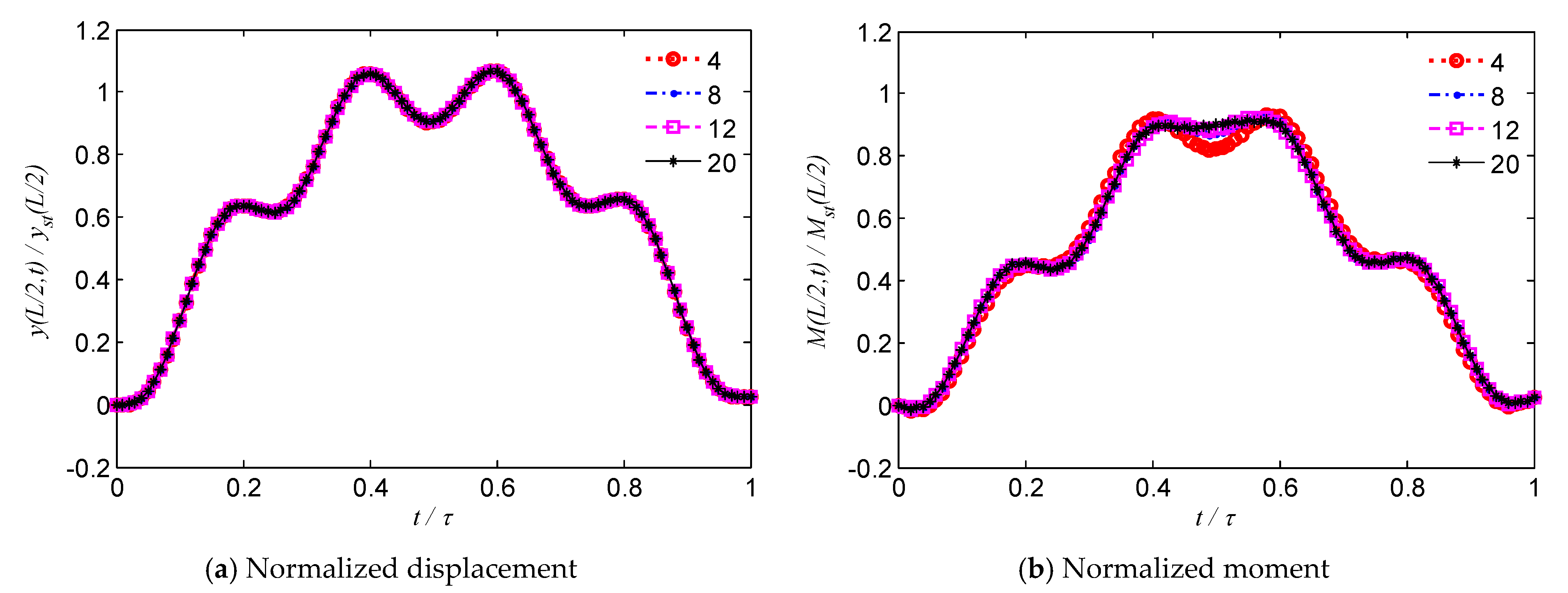
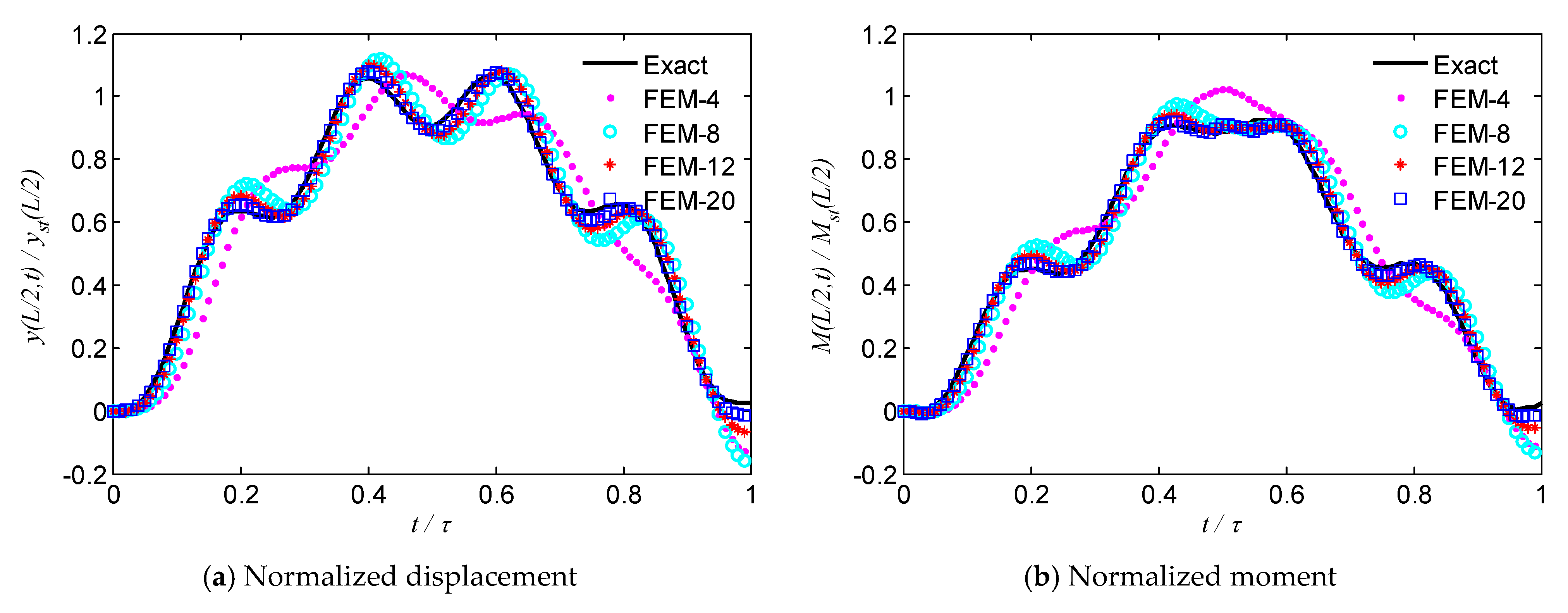
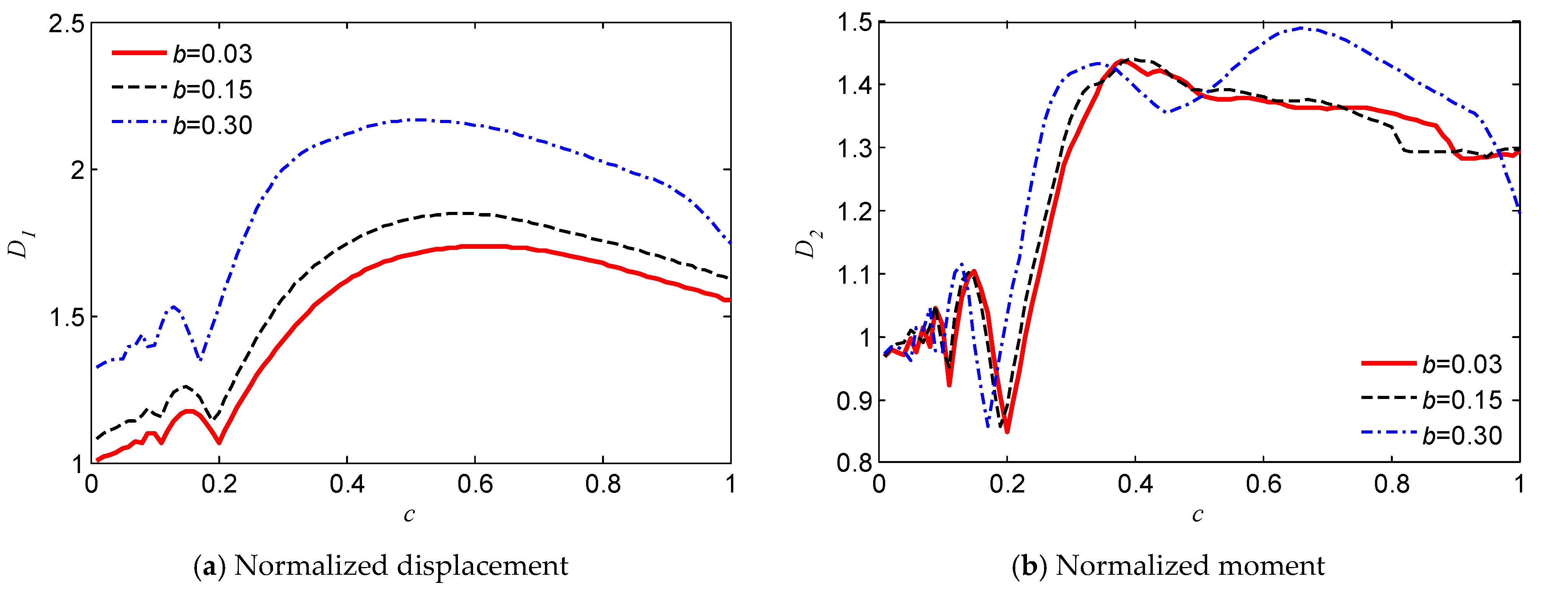
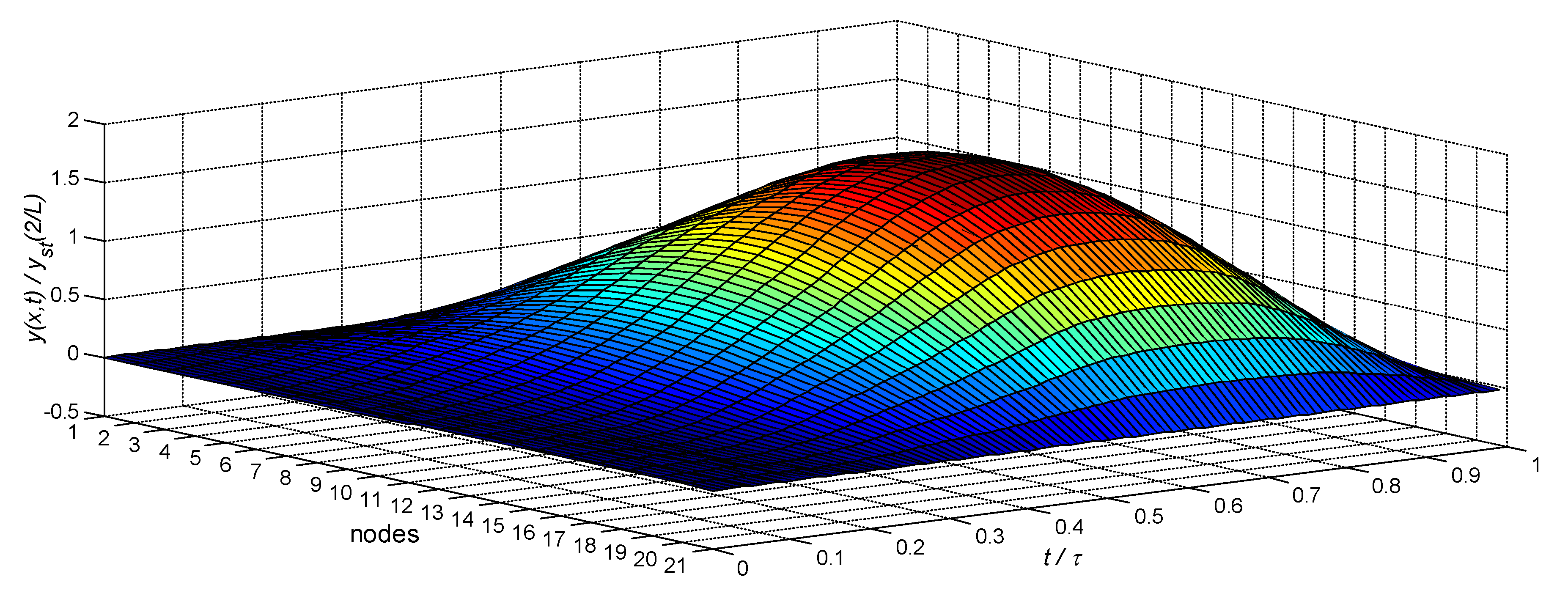
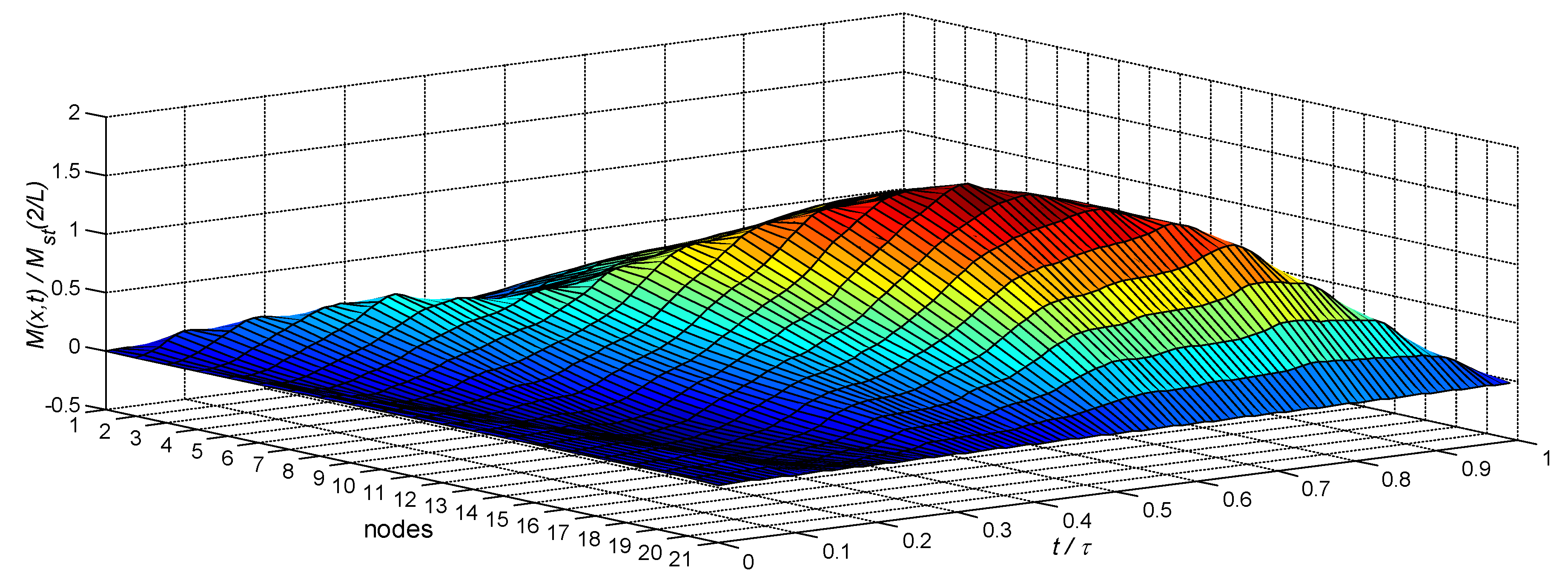
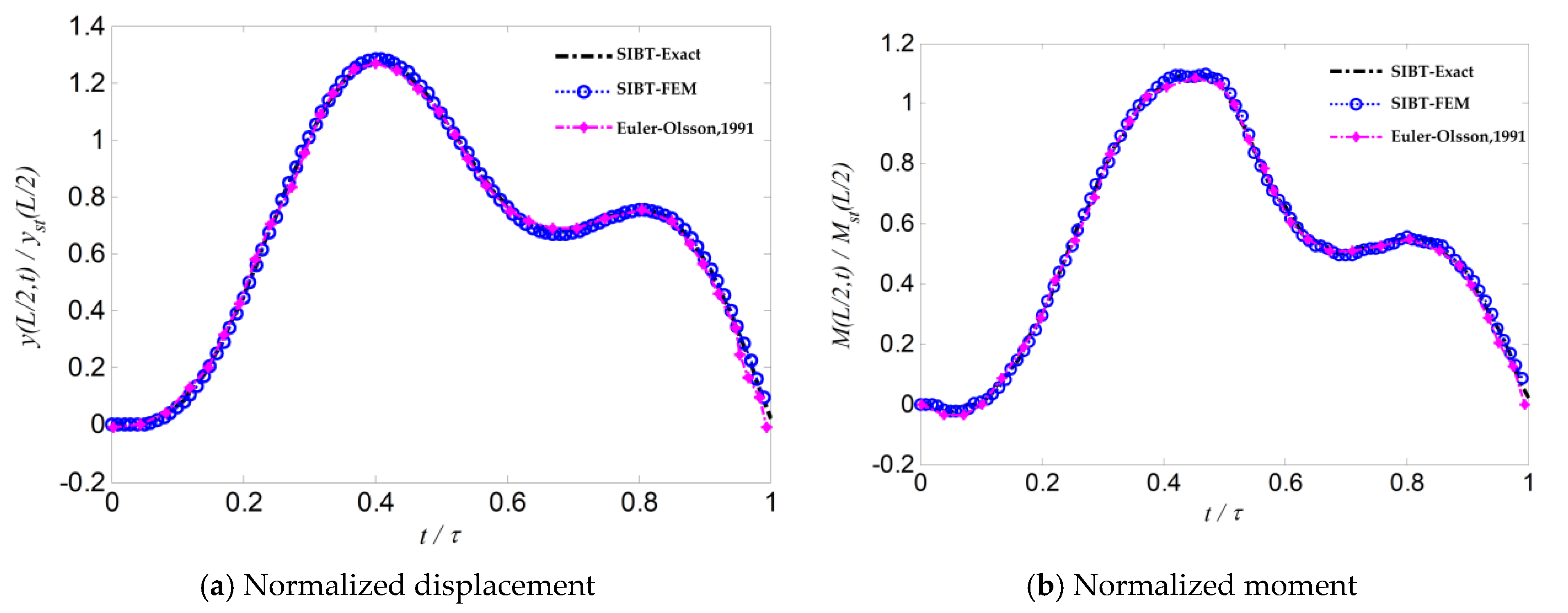
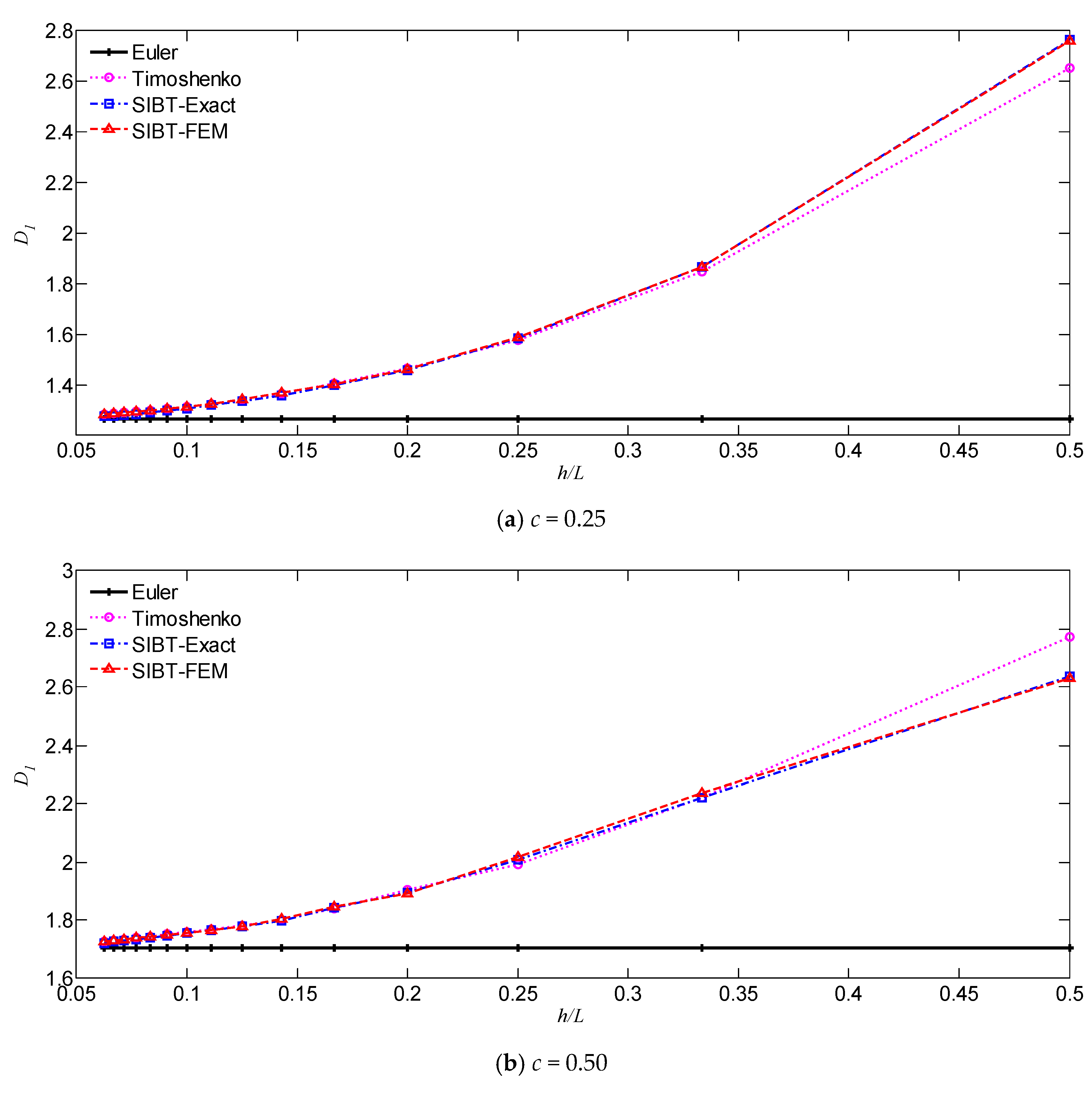
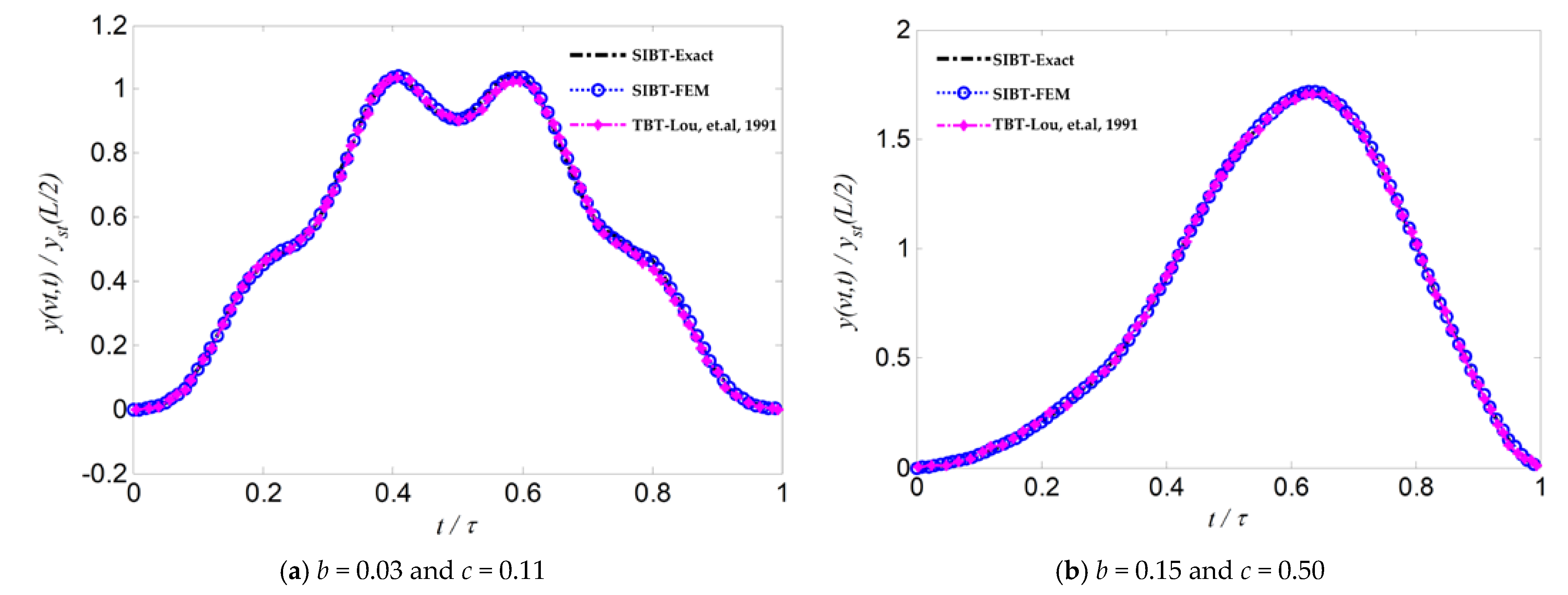
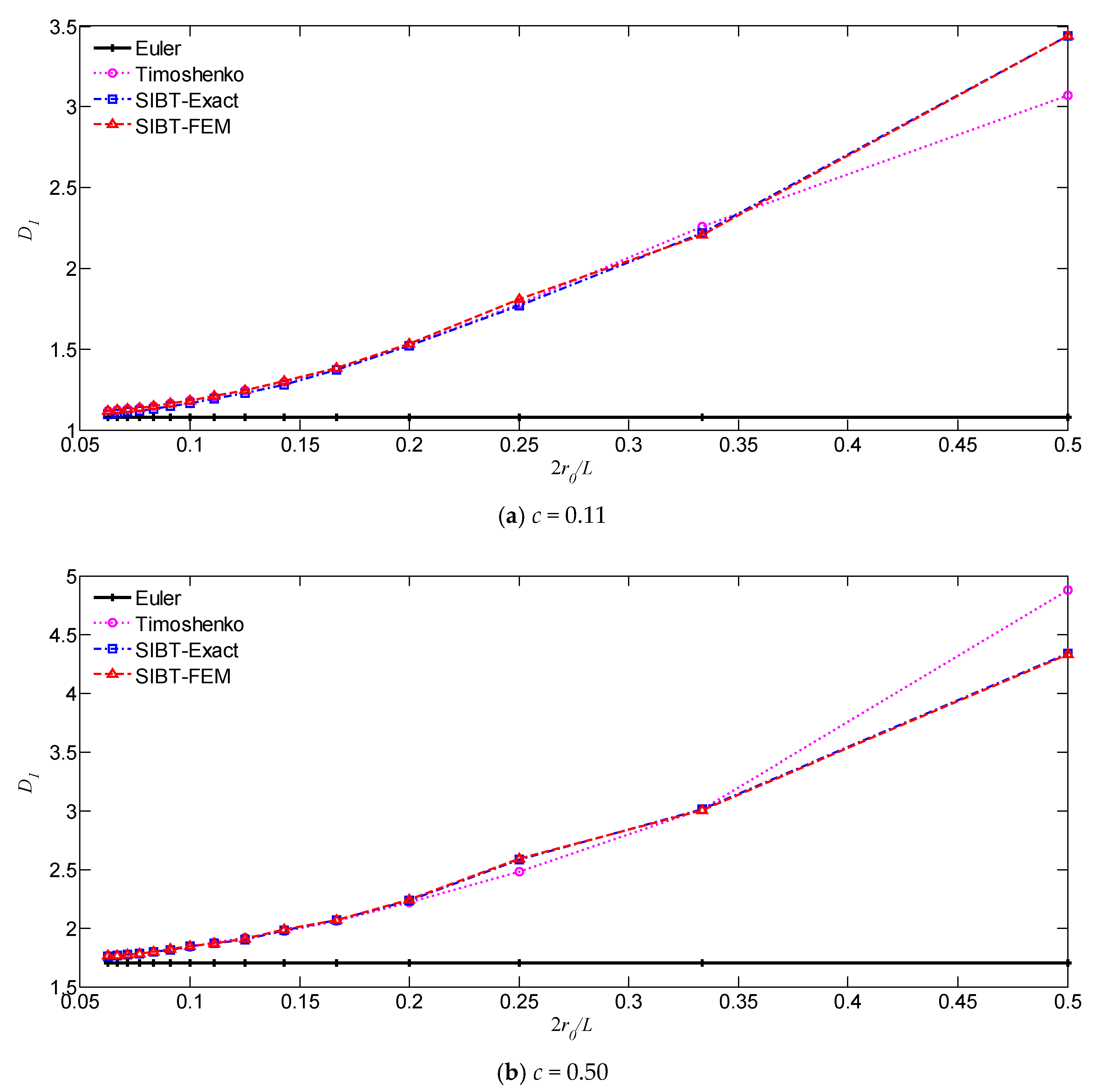
4.4. Numerical Results

The case of a simply supported beam reported in [17,34,35] is considered. The beam is discretized into an even number of elements with equal length and using 100 equal incremental time steps [38].

The numerical results of the normalized mid-span displacement and moment of the beam with b = 0.03 and c = 0.11 discretized into different numbers of elements are plotted in Figure 4. It can be seen that when the number of elements is 20, the numerical results of displacement and bending moment are in good agreement with the analytical results. Therefore, in the following finite element analysis, the beam is discretized into an even number of elements and at least 20.

Figure 5 shows the numerical results of the normalized mid-span deflections and bending moments for various moving speeds of the load. As stated earlier, the critical speed is used as a reference [7,17,34,35,39,40,41]. Note that for the SIBT model, the fundamental frequency ${\omega }_1$ is defined by Equation (17), which is different from ${\omega }_1^{*}={\left(\pi /L\right)}^2\sqrt{EI/\rho A}$. With b = 0.03, one can easily obtain the critical speed parameter $c^{*}$ = 0.998. This means that the velocity of the moving load is just equal to ${\omega }_{1}L/\pi$ and that the ratio between the moving time of the load on the beam and the fundamental period $\tau /T_1$ is 0.5. Five moving speeds are considered here, namely, c = 0.125$c^{*}$, 0.25$c^{*}$, 0.5$c^{*}$, $c^{*}$ and 1.5$c^{*}$. For $c<c^{*}$, as the c increases, the beam displacement response deviates further from the static one. The maximum normalized mid-span displacements are 1.139, 1.269 and 1.710 for c = 0.125$c^{*}$, 0.25$c^{*}$ and 0.5$c^{*}$ respectively. For $c=c^{*}$, the beam displacement response reaches the maximum when the moving load leaves the beam ($t/\tau =1$), and the corresponding maximum displacement amplification factor is 1.554. For $c=1.5c^{*}$, the mid-span displacement increases monotonously with the marching time, and the maximum displacement amplification factor is 1.008. In this case, the maximum response occurs after the moving load has passed the beam, similar to an impact problem [7]. This phenomenon is related to the speed of the waves in the beam. As for the bending moment, the maximum normalized mid-span moment is less than the maximum normalized mid-span displacement. However, the bending moment histories are more irregular.

To further visualize the dynamic character of the beam under the moving load with different speeds, the dynamic magnification factors are carefully presented for the whole range $0.01\le c\le 1.0$ and different cross-sections b = 0.03, 0.15 and 0.30, in Figure 6. The dynamic magnification factors of mid-span displacement and mid-span moment are defined as $D_1=\max [y(L/2,t)/y_{st}(L/2)]$ and $D_2=\max [M(L/2,t)/M_{st}(L/2)]$, respectively. We can clearly see that with the increase in the moving speed of the load, the displacement amplification factor changes nonlinearly, which is associated with the oscillations discussed in Figure 5. In addition, with the increase in the cross-section size of the beam, the displacement amplification factor has a tendency of constant amplification. This phenomenon can be attributed to the increasing influence of the shear effect of the SIBT beam. Compared to the displacement magnification factors $D_1$, we can note that the moment factors $D_2$ are more irregular; $D_2$ is smaller than $D_1$ for all c; and $D_2$ is even less than unity for certain c values. Taking b = 0.03 for an example, the main increases in the factors $D_1$ and $D_2$ occur only in the intervals $0.2\le c\le 0.62$ and $0.2\le c\le 0.38$, respectively. The max ($D_1$) = 1.738 for c = 0.62 and max ($D_2$) = 1.437 for c = 0.38. For lower values of the ratio c, that is $c\le 0.20$, the magnification factors in Figure 6 both increase and decrease with increasing c. For higher c values, $c>0.62$ and $c>0.38$ respectively, $D_1$ and $D_2$ decrease in the present problem.

Figure 7 and Figure 8, respectively, plot the nodal time history of the normalized displacements and bending moments of a beam. For example, the beam with b = 0.03 is subjected to a moving load with c = 0.50. The maximum displacement of the beam is found to be 1.71$y_{st}(L/2)$, occurring at node 11, which locates at the mid-span, and when t = 0.66$\tau$. However, the maximum bending moment of the beam of 1.57$M_{st}(L/2)$ occurs at node 13, which corresponds to x = 0.6 L, and when time t = 0.61$\tau$. This interesting phenomenon shows the discrepancy between the occurrences of the maximum displacement and bending moment. The reason may be related to the assumption of the SIBT, which deserves further study.

5. Comparative Study

Firstly, the dynamic response of a Euler–Bernoulli beam with a square cross section studied in reference [7,39,40,41] is revisited. The magnitude of the moving load P is set to 4.448 N, and the physical properties of the beam are listed in

Table 2. Parameters and properties of the beam.

Parameters	Value
Beam length L	0.1016 m
Young’s modulus E	2.07 × 1011 N/m2
Shear modulus G	7.76 × 1010 N/m2
Shear correction coefficient $k$	5/6
Density $\rho$	10,663 kg/m3
Square cross-sectional area A	4.03 × 10−5 m2
Area moment of inertia I	1.35 × 10−10 m4

. Similarly, for the SIBT model, the critical speed parameter $c^{*}=0.993$.

Figure 9 shows the comparison in terms of dynamic responses of the beam modeled according to the SIBT and Euler–Bernoulli with c = 0.25. It can be seen that time histories of the normalized mid-span displacement and bending moment obtained according to the SIBT model are virtually the same as those calculated by the Euler–Bernoulli model [7]. This is expected in view of the fact that the height–span ratio of the beam is 1:16, which is very small. Consequently, for a slender beam, the effect of shear deformation and shear inertia captured by the SIBT model is negligible.

Table 3. D₁ and D₂ for different moving speeds.

c	D1						D2
	SIBT		Euler-Bernoulli				SIBT		Euler-Bernoulli
	Exact	FEM	[7]	[39]	[40]	[41]	Exact	FEM	[7]	[41]
0.125	1.137	1.151	1.121	1.112	-	1.122	1.038	1.048	1.027	1.031
0.250	1.275	1.284	1.258	1.251	1.258	1.259	1.091	1.097	1.089	1.082
0.500	1.722	1.728	1.705	1.700	1.707	1.706	1.400	1.403	1.389	1.390
0.993	1.570	1.567	-	-	-	-	1.319	1.296	-	-
1.000	1.569	1.560	1.548	1.540	1.547	1.550	1.317	1.287	1.273	1.286

further compares the dynamic amplification factors of the SIBT beam and Euler-Bernoulli beam. As can be seen from Table 3, and referring to Figure 6, with the increase of the moving speed of the load, the displacement and moment amplification factors both change nonlinearly. In addition, although the calculation results of the SIBT beam are generally larger than the calculation results of the Euler–Bernoulli beam, the differences are very small, due to the slenderness of the beam.

To further compare the dynamic responses of the SIBT, Euler–Bernoulli and Timoshenko beams with different slenderness ratios, based on Table 2, the ratio of the cross-sectional dimension to beam length is reset from 1/16 to 1/2. One can find from Figure 10 that, as the ratio of the cross-sectional height h to beam length L increases, the dynamic magnification factors for mid-span displacement obtained by the Euler–Bernoulli always remain 1.266 and 1.706 when c = 0.25 and 0.5, respectively. In contrast, the dynamic magnification factors for mid-span displacement obtained by the SIBT and Timoshenko beams become larger and larger than that obtained by the Euler–Bernoulli beams. Furthermore, until the h/L is greater than 1/3, the difference between the calculated results of the SIBT and Timoshenko beams is apparent. Taking h/L = 1/2 as an example, when c = 0.25, the dynamic magnification factors for the mid-span displacement obtained by the Timoshenko model is 2.652, and that by the SIBT is 2.766. When c = 0.5, the dynamic magnification factors for mid-span displacement obtained by the Timoshenko model is 2.772, and that by the SIBT is 2.638.

Figure 11 shows the dynamic response of the same beam modeled based on the SIBT and Timoshenko models. The mechanical parameters of the beam are listed in Table 1. For comparison purposes, the dynamic magnification factors of displacement and moment here are defined as: $D_3=\max [y(vt,t)/y_{st}(L/2)]$, which means the displacement of the beam is evaluated at the location of the load P during the full moving time. For a Rayleigh parameter b = 0.15, the critical speed parameter $c^{*}=0.958$. As can be seen from Figure 11, the normalized displacement calculated by the SIBT theory is in good agreement with that calculated by the Timoshenko beam theory (TBT). The reason is that although the SIBT takes the effect of shear inertia into account compared with the Timoshenko, the effect of shear inertia is negligible because the beam (with a small value of b) is very slender.

Table 4. D₃ for different cross-section and moving speeds.

c	D3
	SIBT				Timoshenko
	b = 0.03		b = 0.15		b = 0.03	b = 0.15
	Exact	FEM	Exact	FEM	[35]	[35]
0.11	1.044	1.039	1.144	1.149	1.039	1.115
0.3	1.410	1.412	1.557	1.557	1.411	1.555
0.45	1.610	1.611	1.744	1.747	1.610	1.731
0.5	1.602	1.603	1.712	1.715	1.602	1.717
0.7	1.334	1.332	1.368	1.371	1.334	1.366
0.9	1.034	1.034	1.142	1.143	1.034	1.134
0.958	0.979	0.980	1.081	1.085	-	-
0.998	0.946	0.947	1.043	1.045	-	-
1.1	0.873	0.873	0.946	0.949	0.873	0.943
1.3	0.740	0.739	0.776	0.776	0.740	0.777
1.5	0.603	0.602	0.645	0.646	0.603	0.637

compares the results of the beam modelled according to the SIBT and Timoshenko theory. Two beam sections are considered, namely b = 0.03 and 0.15. As the moving speed of the load increases, the displacement amplification factor $D_3$ also changes nonlinearly. When b = 0.03, the calculation results of the SIBT beam are very similar to the results of the Timoshenko beam in the literature. When b = 0.15, the beam is still a slender beam. Although the difference between the results from the SIBT and Timoshenko becomes obvious, the overall difference in the results is not obvious.

Figure 12 further presents the dynamic magnification factors of mid-span displacement of the SIBT, Euler–Bernoulli and Timoshenko beams with different slenderness ratios. Based on Table 1, Rayleigh’s coefficient $b$ is reset from $\pi /32$ to $\pi /4$, while keeping the beam length constant. As the ratio of the cross-sectional diameter to beam length increases, we can draw conclusions similar to Figure 10. For the Euler–Bernoulli beam, the dynamic magnification factors for mid-span displacement remains 1.075 and 1.706 for c = 0.11 and 0.5, respectively. The dynamic magnification factors for mid-span displacement obtained by the SIBT and Timoshenko beams are constantly increasing. Furthermore, until the ratio $2r_0/L$ is greater than 1/3, the difference between the calculated results of the SIBT and Timoshenko beams becomes apparent. This phenomenon is attributed to the significant influence of the shear inertia in the SIBT model.

6. Conclusions

A relatively newly developed beam theory, namely the slope inertia-based Timoshenko (SIBT) beam theory is applied to analyze the dynamic response of a simply supported beam subjected to a moving load. An analytical solution to this problem is presented by using the coupled Fourier and Laplace–Carson integral transformation method.

The finite element solution is also presented and compared with the analytical approach. An excellent agreement is found, thereby implying that the proposed solutions are effective and accurate.

A parametric study is carried out to investigate the difference between the SIBT, Euler-Bernoulli and Timoshenko beam theories for the moving load problem. With the increase of the moving speed of the load, the dynamic magnification factors of the beam displacement and bending moment obtained by the SIBT change nonlinearly, which are related to the dynamic characteristics of the beams. For slender beams, the influence of shear deformation and shear inertia is very small. Therefore, little difference between the dynamic response of the SIBT and that of the Euler–Bernoulli and Timoshenko beams is observed. However, with the increase in the ratio of the cross-sectional size (height or diameter) to beam length, the shear deformation and shear inertia effects are significant, which leads to the dynamic magnification factors for mid-span displacement obtained by the SIBT and Timoshenko beams becoming larger and larger than that obtained by the Euler–Bernoulli beams. Furthermore, until the ratio is greater than 1/3, the difference between the calculated results of the SIBT and Timoshenko beams is apparent.

References

1. Ouyang, H. Moving-load dynamic problems: A tutorial (with a brief overview). Mech. Syst. Signal Process. 2011, 25, 2039–2060. [Google Scholar] [CrossRef]
2. Frýba, L.; Steele, C.R. Vibration of Solids and Structures Under Moving Loads. J. Appl. Mech. 1976, 43, 524. [Google Scholar] [CrossRef]
3. Zhang, X.; Thompson, D.; Sheng, X. Differences between Euler-Bernoulli and Timoshenko beam formulations for calculating the effects of moving loads on a periodically supported beam. J. Sound Vib. 2020, 481, 115432. [Google Scholar] [CrossRef]
4. Xia, G.Y.; Shu, W.Y.; Stanciulescu, I. Analytical and numerical studies on the sope inertia-based Timoshenko beam. J. Sound Vib. 2020, 473, 115227. [Google Scholar] [CrossRef]
5. Aied, H.; Gonzalez, A. Theoretical response of a simply supported beam with a strain rate dependant modulus to a moving load. Eng. Struct. 2014, 77, 95–108. [Google Scholar] [CrossRef] [Green Version]
6. Yang, D.-S.; Wang, C. Dynamic response and stability of an inclined Euler beam under a moving vertical concentrated load. Eng. Struct. 2019, 186, 243–254. [Google Scholar] [CrossRef]
7. Olsson, M. On the fundamental moving load problem. J. Sound Vib. 1991, 145, 299–307. [Google Scholar] [CrossRef]
8. Wu, J.-J.; Whittaker, A.; Cartmell, M. The use of finite element techniques for calculating the dynamic response of structures to moving loads. Comput. Struct. 2000, 78, 789–799. [Google Scholar] [CrossRef]
9. Sun, L. Dynamic displacement response of beam-type structures to moving line loads. Int. J. Solids Struct. 2001, 38, 8869–8878. [Google Scholar] [CrossRef]
10. Basu, D.; Kameswara Rao, N.S.V. Analytical solutions for Euler-Bernoulli beam on viso-elastic foundation subjected to moving load. Int. J. Numer. Anal. Met. 2013, 37, 945–960. [Google Scholar] [CrossRef]
11. Zangeneh, A.; Museros, P.; Pacoste, C.; Karoumi, R. Free vibration of viscoelastically supported beam bridges under moving loads: Closed-form formula for maximum resonant response. Eng. Struct. 2021, 244, 112759. [Google Scholar] [CrossRef]
12. Han, S.M.; Benaroya, H.; Wei, T. Dynamics of transversely vibrating beams using four engineering theories. J. Sound Vib. 1999, 225, 935–988. [Google Scholar] [CrossRef] [Green Version]
13. Timoshenko, S. LXVI. On the correction for shear of the differential equation for transverse vibrations of prismatic bars. Lond. Edinb. Dublin Philos. Mag. J. Sci. 1921, 41, 744–746. [Google Scholar] [CrossRef] [Green Version]
14. Timoshenko, S.P.X. On the transverse vibrations of bars of uniform cross-section. Philos. Mag. J. Sci. 1922, 43, 125–131. [Google Scholar] [CrossRef] [Green Version]
15. Elishakoff, I. An equation both more consistent and simpler than the Bresse-Timoshenko equation. In Advances in Mathematical Modeling and Experimental Methods for Materials and Structures; Springer: Berlin, Germany, 2009; pp. 249–254. [Google Scholar]
16. Chen, Y.H.; Huang, Y.H.; Shih, C.T. Response of an infinite Timoshenko beam on a visoelastic foundation to a harmonic moving load. J. Sound Vib. 2001, 241, 809–824. [Google Scholar] [CrossRef]
17. Lou, P.; Dai, G.-L.; Zeng, Q.-Y. Dynamic Analysis of a Timoshenko Beam Subjected to Moving Concentrated Forces Using the Finite Element Method. Shock Vib. 2007, 14, 459–468. [Google Scholar] [CrossRef] [Green Version]
18. Younesian, D.; Kargarnovin, M.H.; Thompson, D.J.; Jones, C.J.C. Parametrically excited vibration of a Timoshenko beam on random visoelastic foundation subjected to a harmonic moving load. Nonlinear Dynam 2006, 45, 75–93. [Google Scholar] [CrossRef]
19. Nguyen, D.K.; Nguyen, Q.H.; Tran, T.T.; Bui, V.T. Vibration of bi-dimensional functionally graded Timoshenko beams excited by a moving load. Acta Mech. 2017, 228, 141–155. [Google Scholar] [CrossRef]
20. Xia, G.Y.; Zeng, Q.Y. Timoshenko beam theory and its applications. Eng. Mech. 2015, 37, 302–316. (In Chinese) [Google Scholar]
21. Elishakoff, I.; Kaplunov, J.; Nolde, E. Celebrating the centenary of Timoshenko’s study of effects of shear deformation and rotary inertia. Appl. Mech. Rev. 2015, 67, 060802. [Google Scholar] [CrossRef]
22. Elishakoff, I.; Hache, F.; Challamel, N. Variational derivation of governing differential equations for truncated version of Bresse-Timoshenko beams. J. Sound Vib. 2018, 435, 409–430. [Google Scholar] [CrossRef]
23. Nesterenko, V.V. A theory for transverse vibrations of a Timoshenko beam. J. Appl. Math. Mech. 1993, 57, 669–677. [Google Scholar] [CrossRef]
24. Stephen, N.G. The second spectrum of Timoshenko beam theory-further assement. J. Sound Vib. 2006, 292, 372–389. [Google Scholar] [CrossRef] [Green Version]
25. Cazzani, A.; Stochino, F.; Turco, E. On the whole spectrum of Timoshenko beams. Part I: A theoretical revisitation. Z. Angew. Math. Phys. 2016, 67, 24. [Google Scholar] [CrossRef]
26. Cazzani, A.; Stochino, F.; Turco, E. On the whole spectrum of Timoshenko beams. Part II: Further applications. Z. Angew. Math. Phys. 2016, 67, 25. [Google Scholar] [CrossRef]
27. Díaz-De-Anda, A.; Flores, J.; Gutiérrez, L.; Méndez-Sánchez, R.; Monsivais, G.; Morales, A. Experimental study of the Timoshenko beam theory predictions. J. Sound Vib. 2012, 331, 5732–5744. [Google Scholar] [CrossRef]
28. Weaver, W.; Timoshenko, S.P.; Young, D.H. Vibration Problems in Engineering, 5th ed.; John Wiley & Sons Ltd.: New York, NY, USA, 1990. [Google Scholar]
29. Chen, R.; Wang, C.F.; Xue, S.T.; Tang, H.S. Modification of motion equation of Timoshenko beam and its effect. J. Tongji Univ. 2005, 33, 711–715. (In Chinese) [Google Scholar]
30. Elishakoff, I.; Hache, F.; Challamel, N. Critical contrasting of three versions of vibrating Bresse–Timoshenko beam with a crack. Int. J. Solids Struct. 2017, 109, 143–151. [Google Scholar] [CrossRef]
31. Elishakoff, I.; Tonzani, G.M.; Marzani, A. Three alternative versions of Bresse–Timoshenko theory for beam on pure Pasternak foundation. Int. J. Mech. Sci. 2018, 149, 402–412. [Google Scholar] [CrossRef]
32. Bhat, K.S.; Sarkar, K.; Ganguli, R.; Elishakoff, I. Slope-Inertia Model of Non-Uniform and Inhomogeneous Bresse-Timoshenko Beams. AIAA J. 2018, 56, 4158–4168. [Google Scholar] [CrossRef]
33. Chopra, A.K. Dynamics of Structures: Theory and Applications to Earthquake Engineering, 2nd ed.; Tsinghua University Press: Beijing, China, 2005. [Google Scholar]
34. Lee, H. The dynamic response of a Timoshenko beam subjected to a moving mass. J. Sound Vib. 1996, 198, 249–256. [Google Scholar] [CrossRef]
35. Katz, R.; Lee, C.; Ulsoy, A.G.; Scott, R. The dynamic response of a rotating shaft subject to a moving load. J. Sound Vib. 1988, 122, 131–148. [Google Scholar] [CrossRef]
36. Yokoyama, T. Vibrations of timoshenko beam-columns on two-parameter elastic foundations. Earthq. Eng. Struct. Dyn. 1991, 20, 355–370. [Google Scholar] [CrossRef]
37. Reddy, J. On locking-free shear deformable beam finite elements. Comput. Methods Appl. Mech. Eng. 1997, 149, 113–132. [Google Scholar] [CrossRef]
38. Rieker, J.R.; Lin, Y.H.; Trethewey, M.W. Discretization considerations in moving load finite element beam models. Finite Elem. Anal. Des. 1996, 21, 129–144. [Google Scholar] [CrossRef]
39. Yoshida, D.M.; Weaver, W. Finite-element analysis of beams and plates with moving loads. J. Int. Assoc. Bridge Struct. Eng. 1971, 31, 179–195. [Google Scholar] [CrossRef]
40. Filho, F.V. Literature Review: Finite Element Analysis of Structures Under Moving Loads. Shock Vib. Dig. 1978, 10, 27–35. [Google Scholar] [CrossRef]
41. Olsson, M. Analysis of Structures Subjected to Moving Loads. Ph.D. Thesis, Lund University, Lund, Sweden, 1986. [Google Scholar]
Figure 1. Simply supported beam under a moving load P at speed v. Beam length L, cross-sectional area A, moment of inertia I, elastic modulus E, shear modulus G, shear correction coefficient K and mass density ρ.
Applsci 12 03045 g001
Figure 2. Different truncated series solutions of the beam with b = 0.03 and c = 0.11.
Applsci 12 03045 g002
Figure 3. Model of the SIBT beam element with a moving load.
Applsci 12 03045 g003
Figure 4. Numerical solutions with different element numbers of the beam with b = 0.03 and c = 0.11.
Applsci 12 03045 g004
Figure 5. Mid-span displacement and moment of the beam with b = 0.03 and c = 0.125 c * , 0.25 c * , 0.5 c * , c * and 1.5 c * .
Applsci 12 03045 g005
Figure 6. Dynamic magnification factors of the beam under moving load P at different speeds.
Applsci 12 03045 g006
Figure 7. Displacement–time graph at each beam node.
Applsci 12 03045 g007
Figure 8. Moment–time graph at each beam node.
Applsci 12 03045 g008
Figure 9. Mid-span displacement and bending moment of beam with c = 0.25.
Applsci 12 03045 g009
Figure 10. Dynamic magnification factors of the beam with different slenderness ratios.
Applsci 12 03045 g010
Figure 11. Normalized displacement of the beam.
Applsci 12 03045 g011
Figure 12. Dynamic magnification factors of the beam with different slenderness ratios.
Applsci 12 03045 g012