1. Introduction
Refrigerators and air conditioners, as essential household appliances, have a very high prevalence rate around the world. A total of 1.4 billion refrigerators are used, and the annual power consumption exceeds 650 TWh/year [
1]. As the main body of building energy consumption, air conditioner systems account for almost half of building energy consumption and approximately 10–20% of total energy consumption [
2]. Many researchers have conducted extensive studies on refrigeration [
3,
4] and heat pump systems [
5] in order to improve the operational efficiency of refrigeration systems and reduce energy wastage. However, as the core component of refrigerators and air conditioners, hermetic refrigeration compressors directly determine the overall performance and stability of the system. For example, failure of hermetic refrigeration compressors will cause refrigeration system failure, increase noise, reduce service life and reduce COP. Breuker and Braun’s [
6] research showed that compressor failures are by far the costliest failure for refrigeration systems and account for 24% of the costs. Most of the faults already exist in the process of producing equipment. Therefore, it is necessary to diagnose the hidden faults and manufacturing defects of the assembled compressor in the production inspection link. At the same time, the type of manufacturing defect of compressors can be diagnosed, and the cause of the defect can be found. Lastly, the automated production line can be optimized.
In the past, fault diagnosis of hermetic refrigeration compressors often relied on manually identifying abnormalities by touching and hearing. This method is not only wasting manpower, but also makes it difficult to ensure accuracy. To solve this issue, a large number of researchers have studied intelligent fault diagnosis methods for hermetic refrigeration compressors. Cui et al. [
7] used information entropy to analyze signal characteristics and used support vector machines (SVM) to diagnosis the fault of the compressor valve. Deng et al. [
8] used infrared thermal imaging and SVM classifiers to diagnose reciprocating compressors. Farzaneh-Gord et al. [
9] used multiscale sample entropy and global distance for compressor fault diagnosis. These methods can effectively diagnose the type of compressor failure. However, these methods not only require a large amount of a priori knowledge and take a lot of time, but also cannot handle complex data and big data. Since 2010, with the rapid development of data-driven methods represented by deep learning, the above issues have been easily solved. Zhang et al. [
10] realized compressor fault diagnosis with the help of a deep belief network and used ensemble empirical mode decomposition to denoise the original signal. Cabrera et al. [
11] used long- and short-term memory networks to diagnose compressor faults and used a Bayesian network to optimize the parameters of the model. Xiao et al. [
12] constructed deep convolutional neural networks (CNN) to diagnose the fault of the reciprocating compressor air valve. In this paper, CNN are introduced to automatically learn different feature information from the signal of a hermetic compressor for fault classification.
In recent years, many studies have proposed intelligent fault diagnosis methods for rotating machinery based on vibration signals. Xu et al. [
13] used raw vibration signals for fault identification of the fan. Huang et al. [
14] proposed a deep decoupled CNN input as the raw signal to diagnose faults. The time series does not represent the frequency characteristics and displacement variation characteristics of the raw vibration signal. Therefore, a time-frequency processing method is introduced to represent the time-domain and frequency-domain characteristics of the raw vibration signal. Yang et al. [
15] used wavelet transform to extract vibration signal features and used neural networks to classify the fault of reciprocating compressors. Pichler et al. [
16] used the time-frequency method for extracting features and used logistic regression and SVM to diagnose the fault of the compressor valve. Konar et al. [
17] proposed a comparative analysis of the continuous wavelet transform (CWT) and the Hilbert transform while using a genetic algorithm for fault diagnosis of asynchronous motors. Verstraete et al. [
18] compared the feature extraction capabilities of short-time Fourier transforms (STFT), CWT and Hilbert-Huang transform (HHT), and finally used CNN for fault diagnosis. These methods demonstrate that the time-frequency processing method has strong feature extraction capability.
The time-frequency processing method can improve the stability of the diagnosis algorithm. It is difficult to find a method with absolute advantages because different time-frequency processing methods have different advantages for the compressor vibration signals. To avoid the disadvantage that a single type of time-frequency processing method cannot express the rich information in the raw vibration signal, this paper proposes a dual time-frequency image fusion method based on convolutional neural network for compressor manufacturing defect diagnosis. This method realizes the fusion and complementation of different time-frequency information and makes full use of the image feature recognition ability of the deep neural network. The main contributions of the paper can be summarized as follows:
(1) The proposed method uses CWT and HHT for feature extraction of the same raw vibration signal, and the extracted features are complementary. The proposed method achieves richer feature extraction for a single vibration signal and ensures the accuracy of diagnosis.
(2) The proposed method constructs a dual-channel fusion convolutional neural network that can effectively learn manufacturing defect features from two time-frequency images and fuse them to realize an end-to-end diagnosis of compressor manufacturing defect based on the time-frequency image of the vibration signal.
(3) A large number of experiments verified the differences between different time-frequency processing methods and different classification models and proved the superiority of the proposed method with higher diagnostic performance and robustness.
The rest of this paper is organized as follows:
Section 2 introduces the feature extraction method—dual time-frequency images fusion.
Section 3 presents a diagnosis method of hermetic refrigeration compressors based on dual time-frequency images fusion.
Section 4 introduces the experimental setup and data processing.
Section 5 gives the experimental results and comparative study, and
Section 6 concludes the paper.
2. Feature Extraction Method—Dual Time-Frequency Images Fusion
2.1. Data Preprocessing
The time-domain signal of the compressor shows less characteristic information because the coupling between the fluid flow and the mechanical structure of the hermetic refrigeration compressor causes the vibration signal to have complex characteristics. It is necessary that the vibration signal is transformed in the time-frequency domain to obtain richer feature information. Time-frequency transform methods, such as Wigner-Ville distribution (WVD) [
19], short-time Fourier transform (STFT) [
20], continuous wavelet transform (CWT) [
18] and Hilbert-Huang transform (HHT) [
21], have been widely used to extract feature from vibration signal. However, WVD and STFT are hindered by low time-frequency concentration and cross-term interference, and they also need additional expertise and prior knowledge to identify the fault features [
22,
23]. The most widely used methods are CWT and HHT. In the following, the principles of the two time-frequency transformations are introduced in detail.
2.1.1. Continuous Wavelet Transforms
The continuous wavelet transform (CWT) has higher time resolution and lower frequency resolution at high frequencies and has lower time resolution and higher frequency resolution at low frequencies, which exhibits multiresolution analysis characteristics. The CWT implements the wavelet transform, which is used to analyze nonperiodic signals and transient signals at different scales or resolutions. The CWT of the signal
is defined as:
where
represents the conjugate transpose of the mother wavelet function
,
is a scale factor,
is the translation factor and
represents the energy normalization across the different scales.
2.1.2. Hilbert-Huang Transform
The Hilbert-Huang transform (HHT) is NASA’s designated name for the combination of empirical mode decomposition (EMD) [
24] and Hilbert spectral analysis (HAS). The HHT analysis process is implemented in two steps: the first step uses EMD to pre-process the data, and the original data are decomposed into a set of finite intrinsic mode functions (IMF); the second step is the Hilbert transform (HT) of the decomposed IMF to obtain energy-frequency-time distribution.
The EMD decomposes any signal in the IMFs as follows: For any data sequence,
and
, the local maximum and local minimum of the raw signal, are interpolated by cubic splines to form the mean value of the upper and lower envelopes. The difference between the signal and
is defined as component
:
This process can be repeated
times until
is a basic mode component:
Then the first prototype component
obtained from the raw data is:
After sorting out
from the raw data:
Since still contains information of longer period components, is still treated as new data and processed as described above. This strategy can process all subsequent remaining components . The sifting process ends when the preset stoppage criterion is satisfied. The stoppage criterion can be set as follows: when the remaining component becomes smaller than a predetermined value or when the remaining component becomes a monotonic function. The EMD algorithm is based on the local characteristics of the signal, and the basic mode components and residual components are obtained by iterative screening of the local mean. It can be explained that the decomposition and reconstruction of the signal have advantages, such as reducing noise interference and eliminating data.
According to the definition of HT, the HT of real function
is the real-valued function, which is defined as:
Here, the
P indicates the principal value of the singular integral. An analytical signal was
, consisting of
and
in the complex number of
.
Here,
is the amplitude of the analytical signal, and
is the phase of the analytical signal.
Therefore, according to the definition, the instantaneous frequency expression is:
The polar coordinate expression shown in Equation (7) further emphasizes the local characteristics. It can be seen from this expression that both amplitude and phase are functions of time, and these form the basis of signal expression in the time domain.
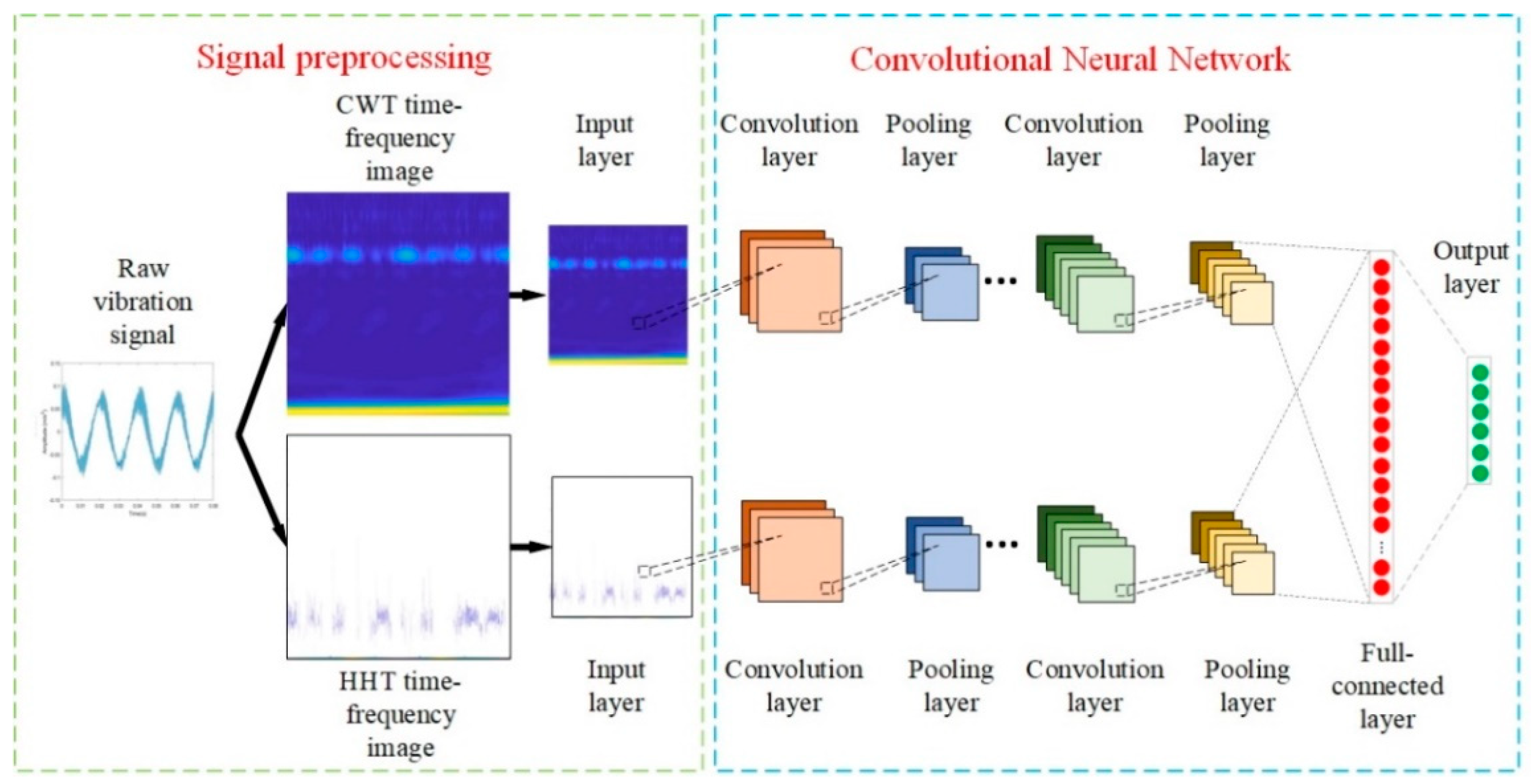
2.2. Establishment of Dual Time-Frequency Images Fusion
According to the above part, it can be seen that the principles of the two time-frequency transformation methods are different, so the extracted features are complementary in the dual time-frequency images. To extract more features and improve the diagnosis accuracy of compressor manufacturing defects, this paper proposes a dual time-frequency image fusion method, and its structure is shown in
Figure 1. The inputs of two parallel convolution and pooling layers are different time-frequency images, and the output is the one-hot label of the input image. The CNN has been successfully applied in various aspects such as image processing [
25] and speech recognition [
26].
Figure 1 shows that the proposed method structure consists of signal preprocessing and CNN. In the signal preprocessing part, CWT and HHT are performed on the same raw vibration signal to obtain two time-frequency images, which reshape to be 128 × 128 pixels. The CNN comprises two parallel convolution and pooling modules, two fully connected layers and an output layer. First, two parallel convolution and pooling modules extract features from dual time-frequency images, respectively.
Feature maps can be obtained in the convolutional layer by convolving the input images with multiple convolutional kernels. The results are input into the activation function. The formula is as follows:
Here, represents the output of the -th convolutional surface of the convolutional layer; represents the weight matrix corresponding to the -th convolution kernel; represents the input matrix; represents the bias term; and represents the activation function. We chose the most widely used activation function ReLU.
For the pooling layer, this paper chooses the maximum pooling. The formula is as follows:
Here, represents the -th pooling layer, represents the block of the output matrix of the previous convolutional layer and represents the dimension of sub−block of the output matrix of the previous convolutional layer. The pooling layer often follows the convolution layers. The pooling layers play the role of quadratic feature extraction, feature dimensionality reduction and limited feature selection.
Secondly, two parallel convolution and pooling modules extract CWT time-frequency image and HHT time-frequency image features, which spliced in the first fully connected layer. Therefore, this process shows realistic feature fusion.
The calculation formula of the fully connected layer is as follows:
Here, represents the output; represents input; represents the weight matrix; represents the bias term; and represents the ReLU activation function.
The fusion stage is implemented by feeding all the extracted dual time-frequency images features into a full-connected layer where the process of feature fusion is realized. The fully connected layer passes the output value to the output layer for classification. The expression of the softmax function of the output layer is as follows:
Here, represents the -th output in the fully connected layer; represents the probability of the corresponding manufacturing defect types corresponding to the -th outputs.
The method of “Dropout” [
27] is introduced within the fully connected layer to prevent over-fitting during classification. During training, some neuron in the hidden layer is stopped. This improves the network’s capability to generalize and prevents overfitting.
According to the above section, the proposed method consists of four convolutional layers and pooling layers, two connected layers and a Softmax layer. We used cross-entropy loss function and Adam [
28] optimization function to train the model. The learning rate is 0.001. This optimizer is suitable for models with many parameters, extensive data and small calculation memory requirements. The weights and biases of the local convolutional and fully connected layers are all trained together through backpropagation. The parameters of the proposed method are shown in
Table 1, where
represents the
-th channel.
5. Experiment Result and Comparative Study
Extensive research has been carried out to prove the superiority of the proposed method. In
Section 5.1, the similarities and differences between the time-domain diagram and time-frequency image of typical manufacturing defects are introduced, proving that it is difficult to diagnose types of manufacturing defects.
Section 5.2 uses confusion matrix and t-distributed stochastic neighbor embedding (t-SNE) to demonstrate the classification ability of the proposed method. In
Section 5.3, four evaluation indicators are used to evaluate different diagnostic methods to illustrate the superiority of the proposed method.
5.1. Experimental Data for Typical Manufacturing Defects
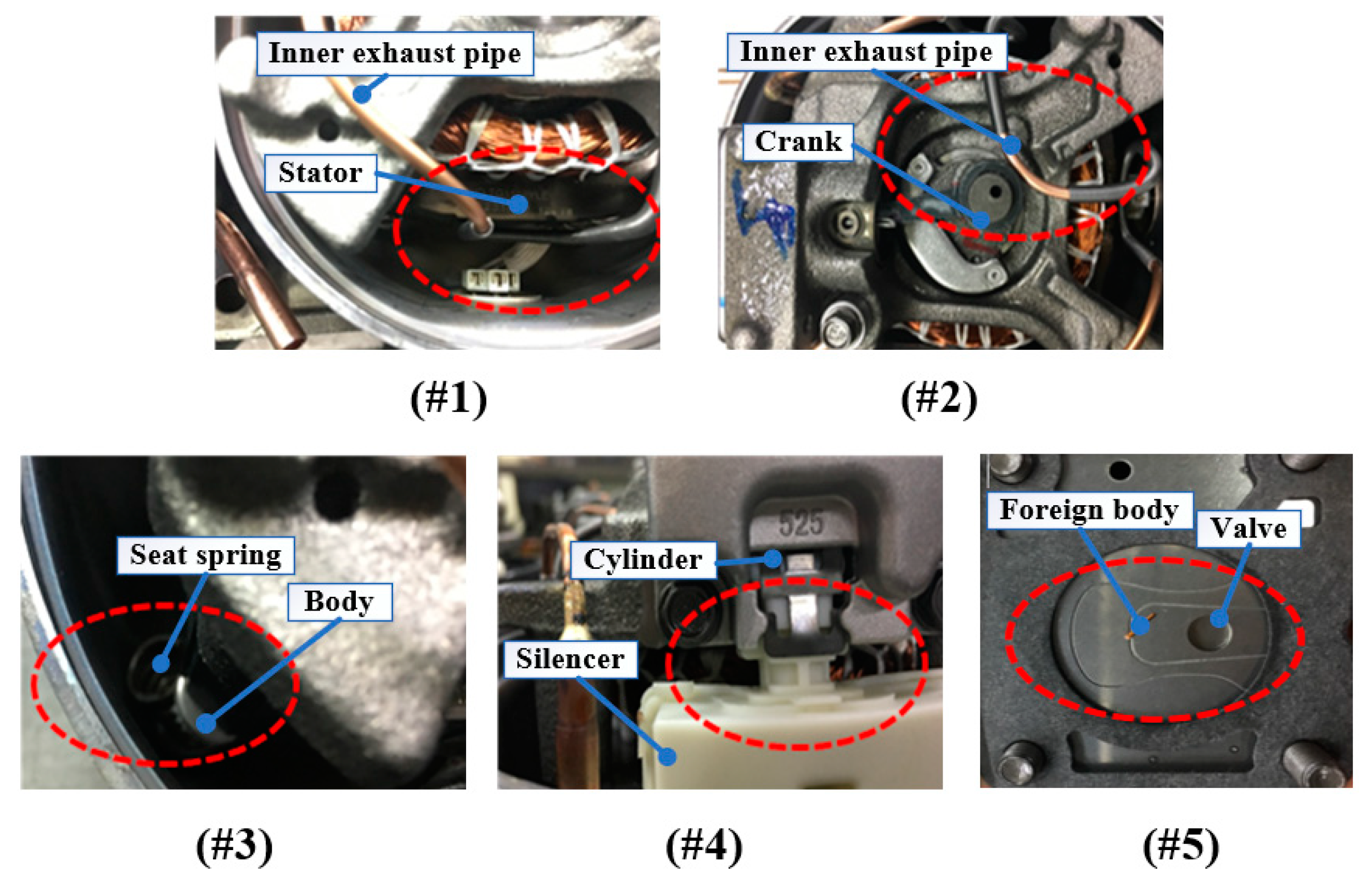
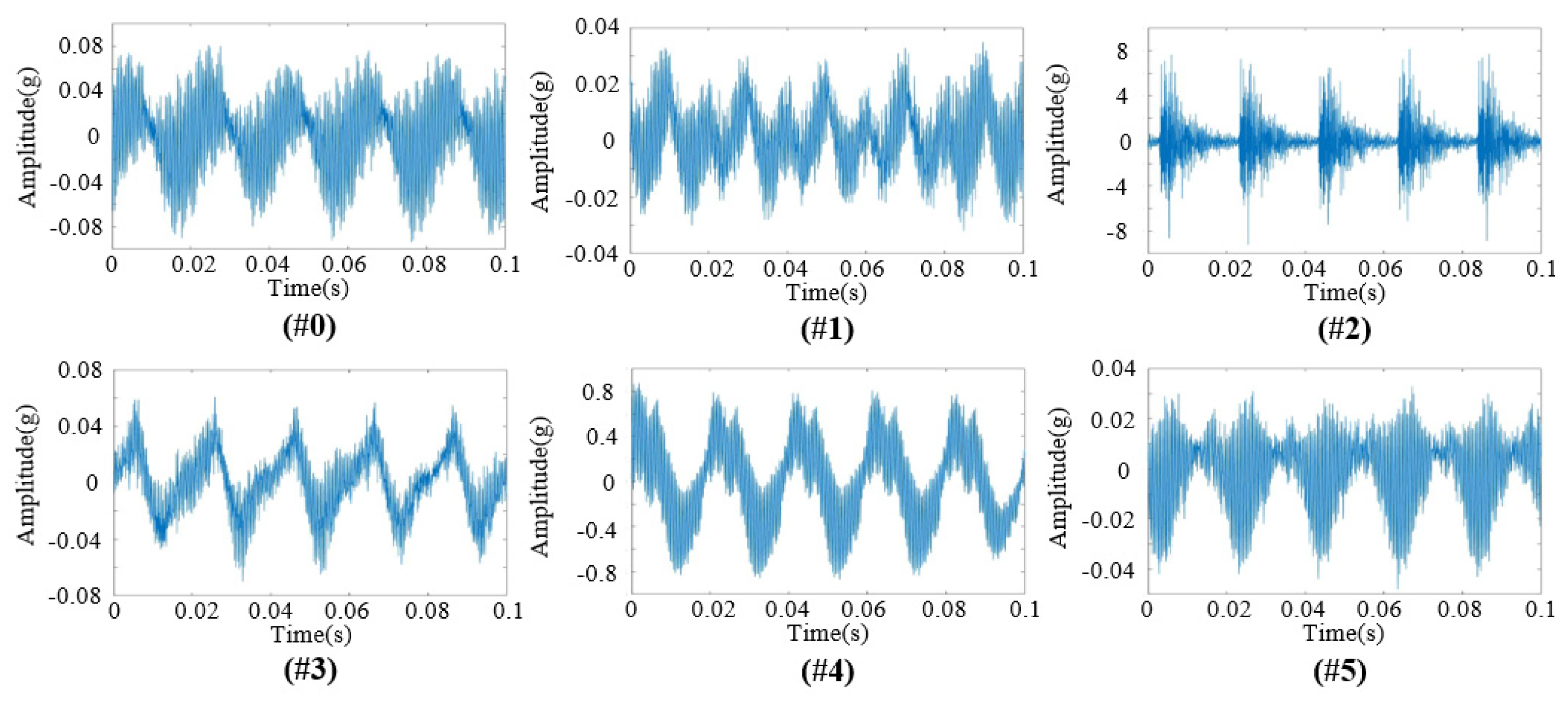
Hermetic refrigeration compressors have a complex structure and many excitation sources. The raw vibration signals of six typical hermetic refrigeration compressors manufacturing defects are shown in
Figure 5. It can be observed seen that the amplitude of #2 and #4 are 8 g and 0.8 g, respectively. The amplitudes of the other four typical manufacturing defect compressors are similar except for #2 and #5; the time-domain diagram of the vibration signal depicts a sine wave.
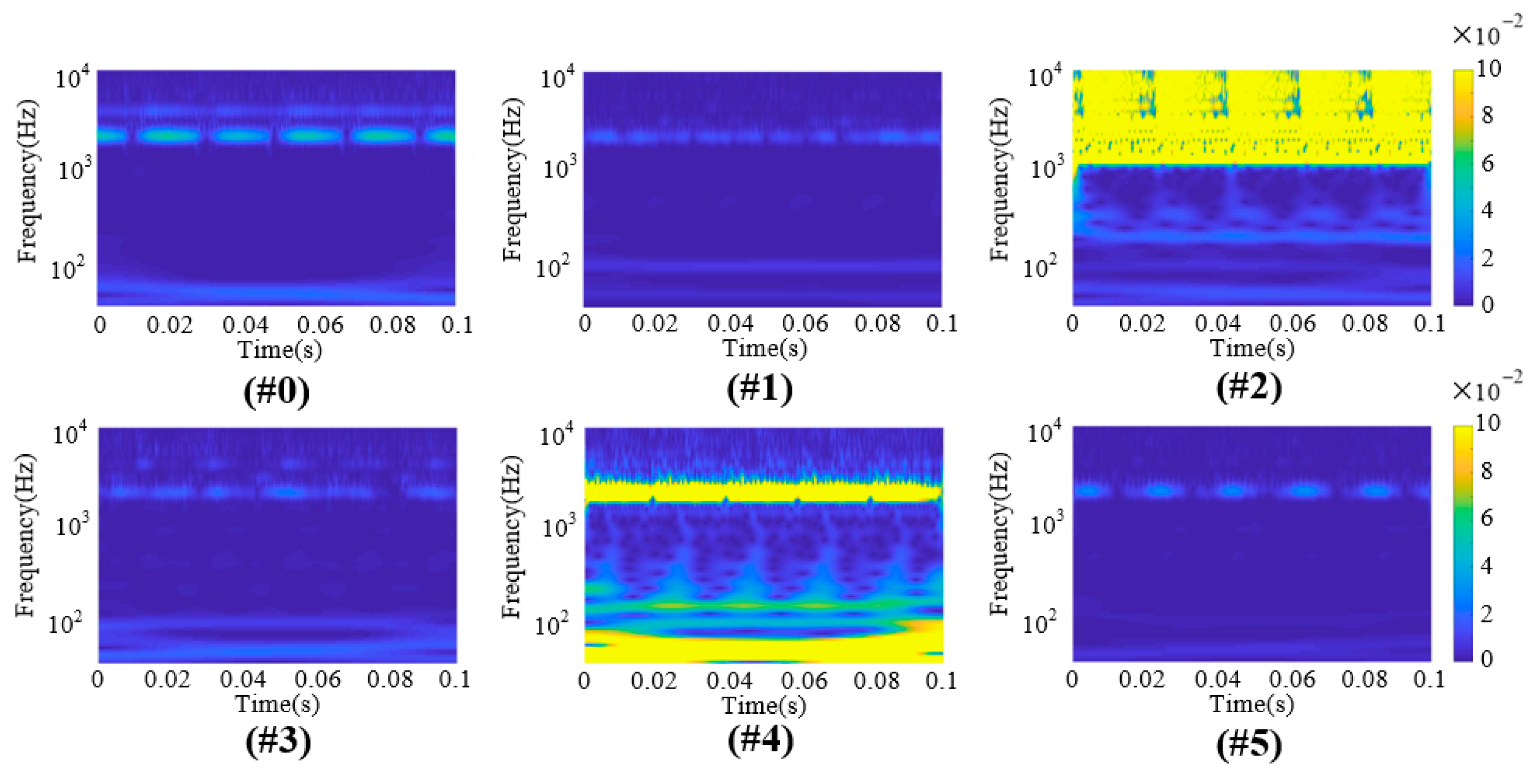
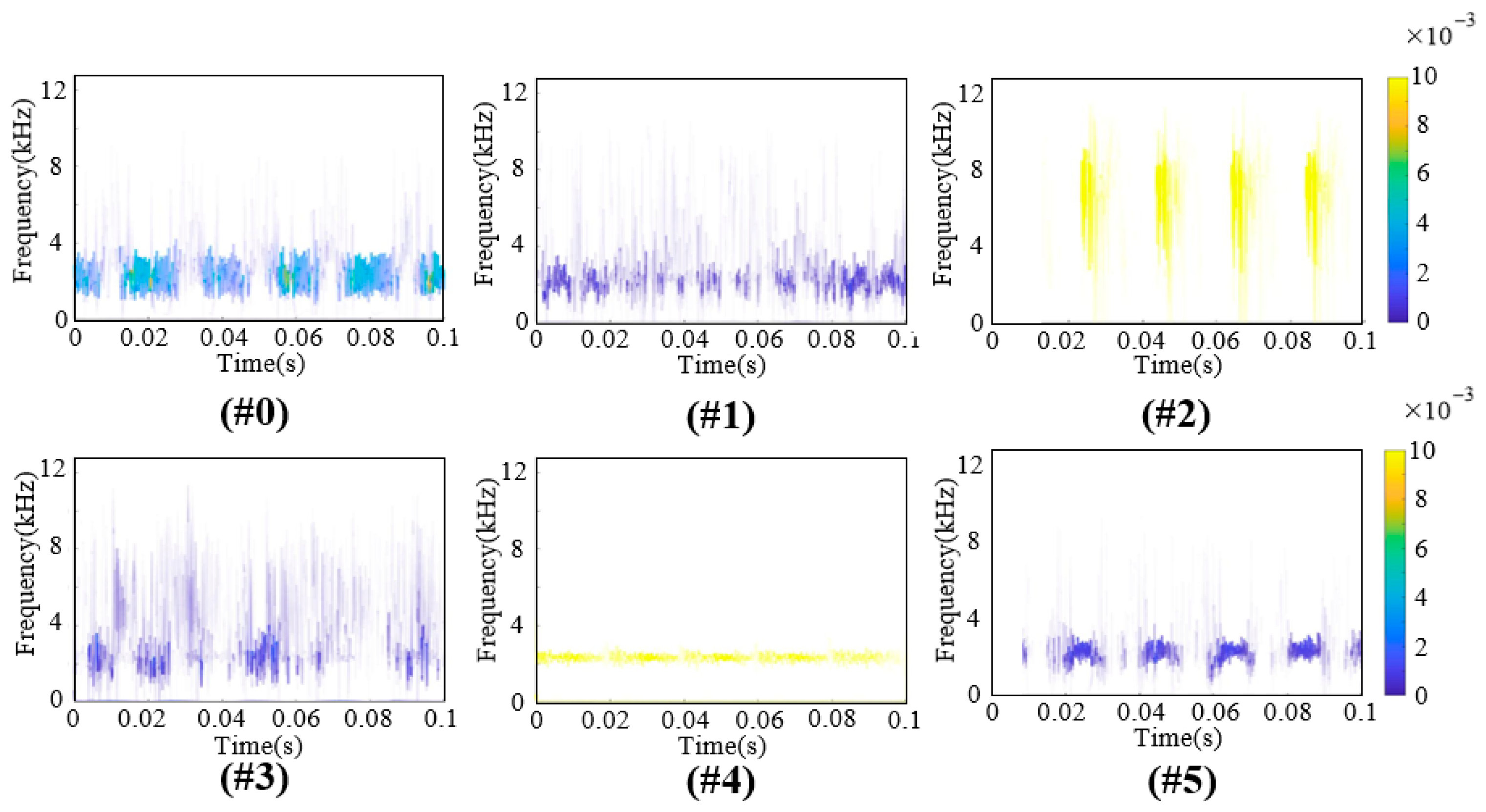
A time-frequency image is a two-dimensional data matrix that carries more information in the time and frequency domains than a one−dimensional signal. The raw vibration signals are transformed by CWT and HHT, and the time-frequency images are shown in
Figure 6 and
Figure 7. Notably, the CWT time-frequency image shows more features in the low-frequency part, and the HHT time-frequency image shows more features in the high-frequency part. It can be demonstrated that the features of two time-frequency images are complementary. It can be observed that the CWT time-frequency image has obvious frequency bands, while the HHT time-frequency image has apparent aliasing phenomena.
Figure 6 and
Figure 7 show that the magnitude of the energy in the time-frequency image is proportional to the amplitude of the vibration signal. It can be seen that the time-domain diagram and the time-frequency images of some typical manufacturing defect compressors are very similar. The time-frequency characteristics of the two hermetic refrigeration compressors are different in the same type of manufacturing defect. Therefore, it is challenging to diagnose the manufacturing defects of hermetic refrigeration compressors by traditional methods.
5.2. The Performance of the Proposed Method
In this part, the performance of the proposed method is discussed for the diagnosis of each manufacturing defect. The testing set for each type of manufacturing defect has 300 samples. The testing results of the proposed method are presented by confusion matrix and t-SNE.
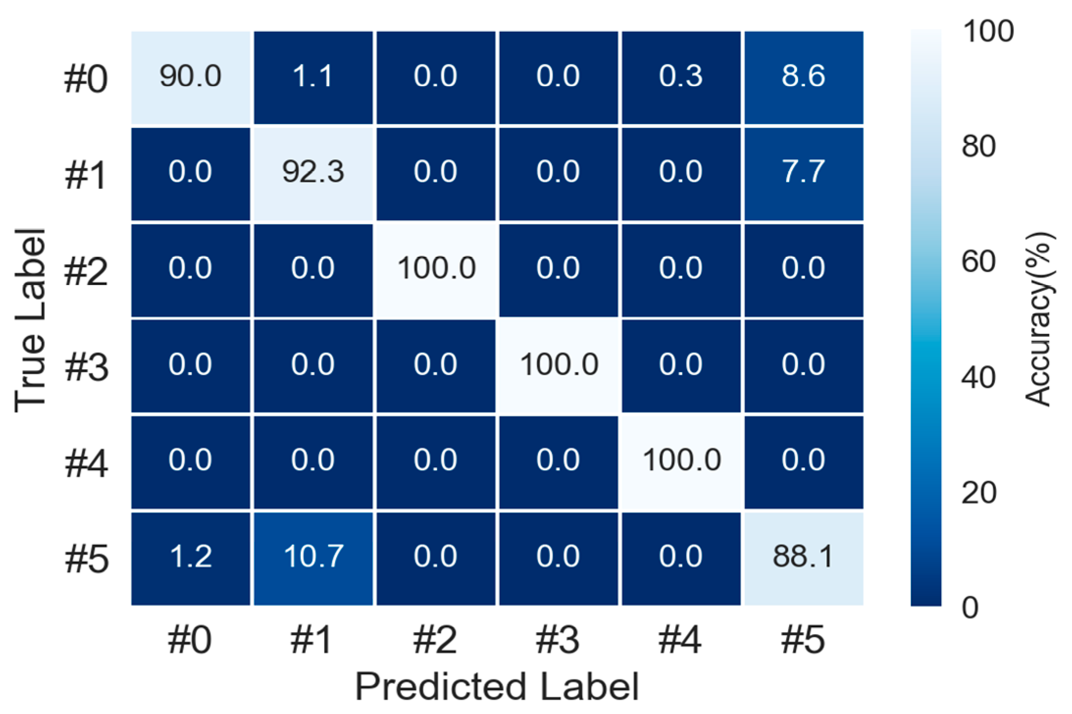
The confusion matrix of the proposed method is recorded ten times, and the average value is shown in
Figure 8.
Figure 8 clearly shows that the diagnostic accuracy of the #2, #3 and #4 are 100%; the diagnostic accuracy of the #0, #1 and #5 are 90%, 92.3% and 88.1%, respectively. It can be seen that most of the misclassified samples of #0 and #1 are diagnosed as #5, and the misclassified sample of #5 is diagnosed as #0 and #1. It can be proved that the proposed method can extract different features for classification in #2, #3 and #4. The extracted features of the proposed method are very similar in #0, #1 and #5. It can be proved that the data description of typical manufacturing defects is correct in the previous part.
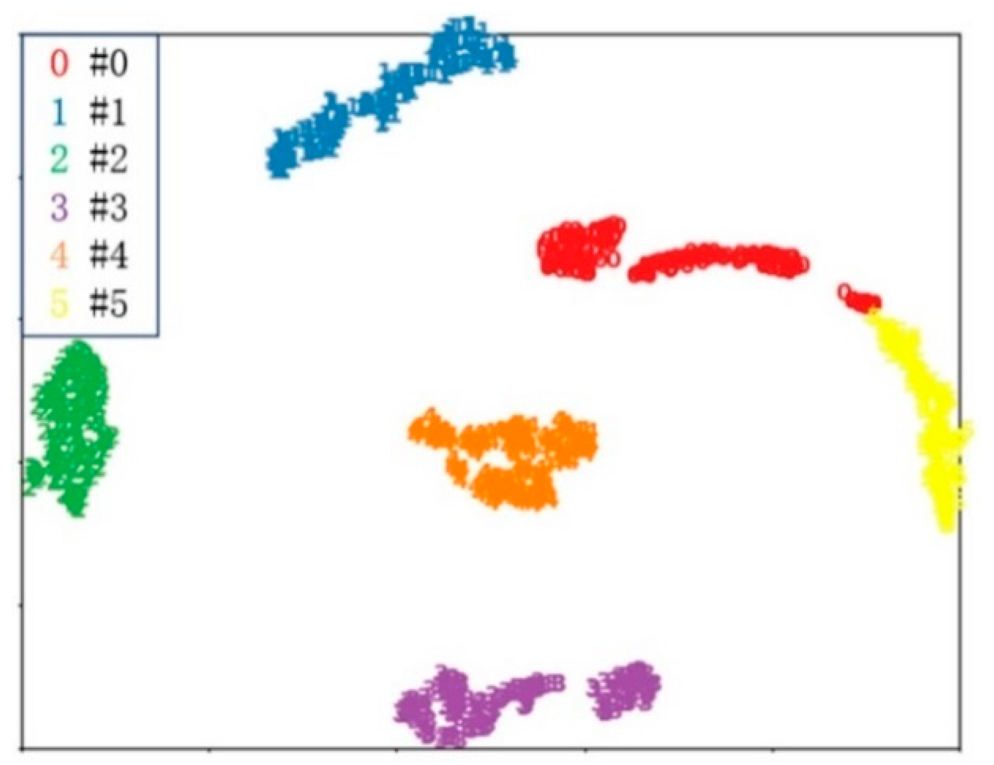
The “t-SNE” can express the feature extraction ability of the model and analyze the clustering of features more intuitively. The visualization tool “t-SNE” implements high-dimensional feature mapping to visualize the learned characteristics, as shown in
Figure 9.
In
Figure 9, it can be seen that the proposed model effectively learned feature information, which helps diagnose and classify a manufacturing defect, and high-level features show prominent clustering characteristics. It is concluded that the proposed method has better diagnostic performance and learned characteristics capabilities.
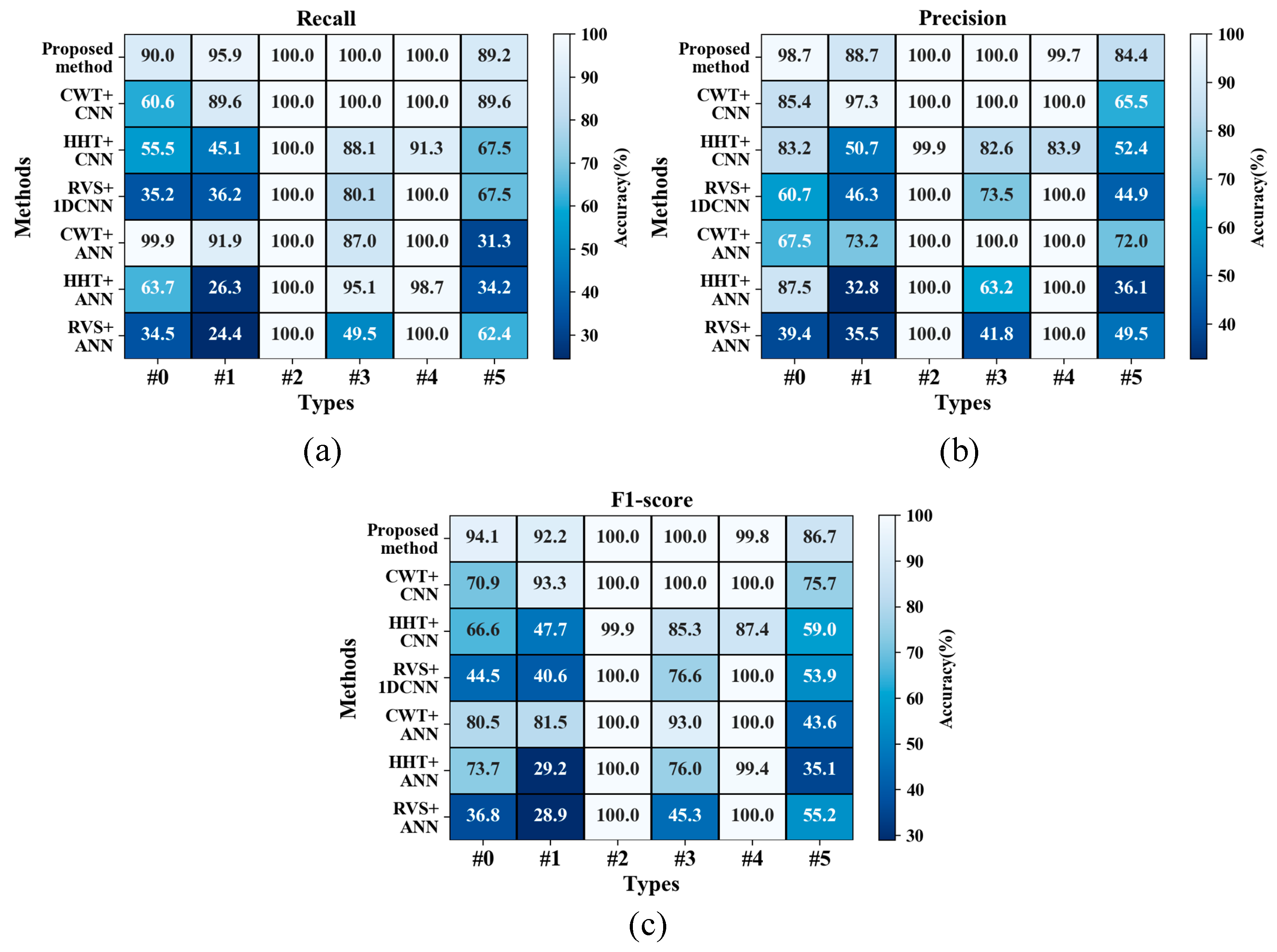
5.3. Comparison of Different Methods
In this part, to further illustrate that the proposed method has high diagnostic performance, the four different evaluation indexes of the proposed method are compared with those of other methods. Evaluation indicators include average
Accuracy,
Precision,
Recall and
F1-
score. The formulae for average
Accuracy,
Precision,
Recall and
F1-
score are (18)–(21).
Take #0 as an example: |TP| represents the number of samples classified correctly into #0, |TN| represents the number of samples classified correctly into other defects, |FP| represents the number of samples classified incorrectly into #0 and |FN| represents the numbers of samples in #0 classified into other classes. The F1-score is used to reflect the overall indicator comprehensively. Here are six different comparison methods:
- (1)
Artificial neural network (ANN) using raw vibration signals (RVS) as input (RVS + ANN);
- (2)
ANN using HHT time-frequency images as input (HHT + ANN);
- (3)
ANN using CWT time-frequency images as input (CWT + ANN);
- (4)
One−dimensional CNN using RVS as input (RVS + 1DCNN);
- (5)
CNN using HHT time-frequency images as input (HHT + CNN);
- (6)
CNN using CWT time-frequency images as input (CWT + CNN);
The input shapes and parameters of the other methods are shown in
Table 3. Different methods record ten trials of diagnosis accuracy, and the average accuracy is utilized to quantify the method, as shown in
Table 3. The other evaluation indicators of the different methods are shown in
Figure 10 for each type of manufacturing defect.
Table 3 shows that the proposed method yields the highest accuracy up to 95.9%, training time is 104 s for 7200 samples and testing time of each sample is 0.1314 s. Therefore, it can be calculated that the proposed method can test 465 samples per minute. Comparing the diagnostic accuracy of different classifiers shows that the diagnostic accuracy of CNN is significantly higher than that of ANN. It can be explained that the CNN, as a deep model, is competent to fuse features in depth and extract more valuable features for compressor manufacturing defect diagnosis. Comparing the diagnostic accuracy of different preprocessing methods shows that the diagnostic accuracy of the HHT and CWT methods is higher than that of the RVS method because the time-frequency image can show more features than the raw vibration signal for manufacturing defect diagnosis. The training time of the proposed method is only lower than that of the HHT + ANN method and CWT + ANN method. The testing time of each sample of the proposed method is larger than that of other methods, but the test rate meets the requirements of the production line.
Figure 10 clearly shows that the evaluation indicator of the proposed method is generally better than that of the other methods for each typical manufacturing defect. A detailed analysis of #0 shows that the recall of CWT + ANN is 9.9% higher than that of the proposed method. However, the precision of CWT + ANN is 31.2% lower than that of the proposed method in #0. From the analysis of CWT + ANN, it can be observed that a small number of normal compressor (#0) samples are misdiagnosed as other defects, but some defective compressor samples are misdiagnosed as #0. If the faulty samples are misdiagnosed as normal samples, it may lead to the failure of the refrigeration system. Thus, it is unreliable to rely only on recall and precision to evaluate the model. The F1-score is an evaluation index that combines the two indicators and comprehensively reflects the overall indicator. It can be seen from
Figure 10c that the F1-score of the proposed method is 13.6% higher than that of the CWT + ANN for #0. A detailed analysis of #3 and #5 reveals that recall, precision and F1-score of the proposed method are higher than that of other methods. The recall, precision and F1-score of each typical manufacturing defect are mostly greater than 90%. It can be proved that the performance of the proposed method is superior to other methods for the diagnosis of compressor manufacturing defects. Since the dual time-frequency image features extracted can be complementary, the proposed methods obtain richer features and higher diagnostic performance.
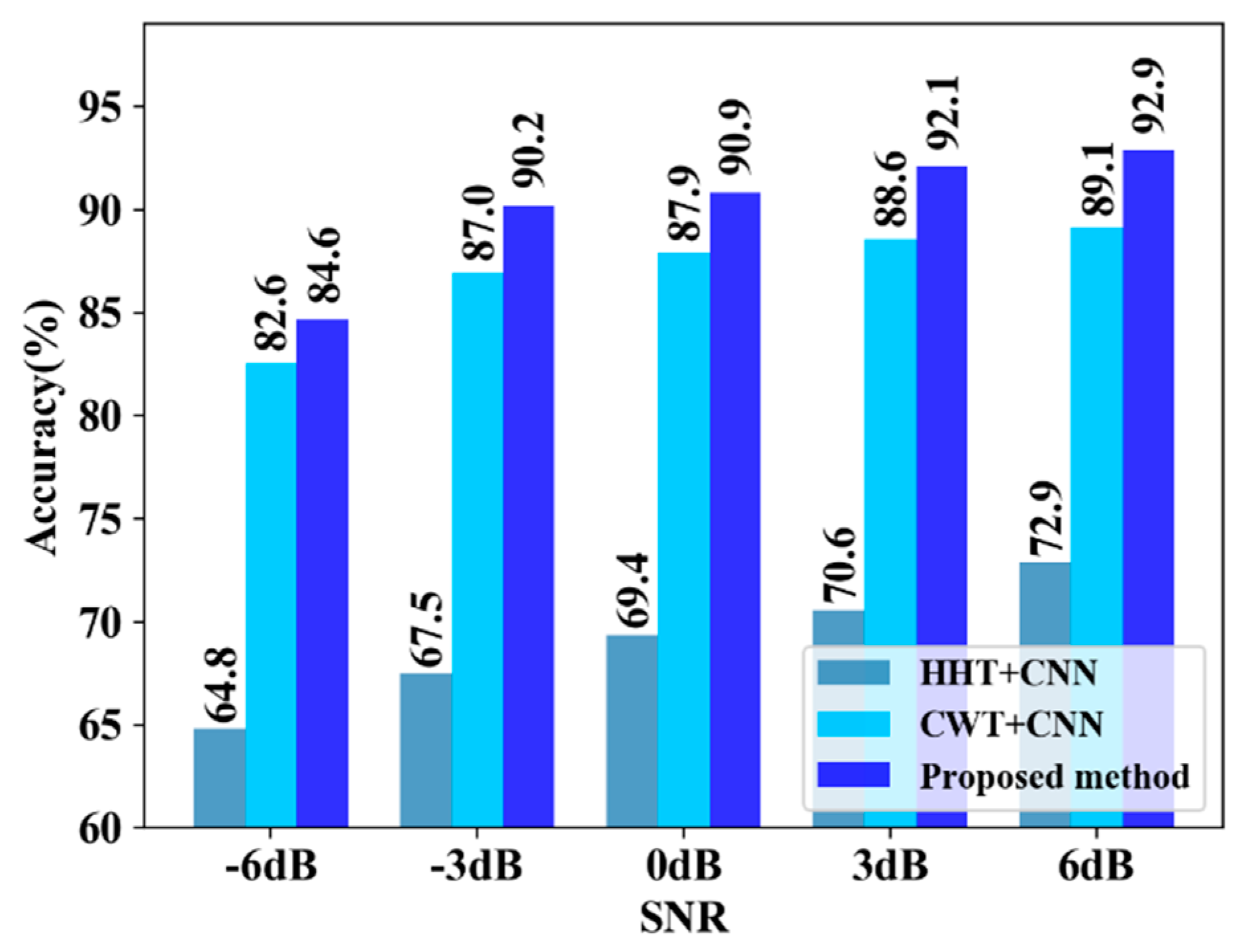
The hermetic refrigeration compressor usually is tested in varying ambient noise levels. Therefore, it is necessary to study the diagnosis performance of the proposed methods under various conditions with a low signal-to-noise ratio (
SNR). Robust fault diagnosis of rotating machinery is realized at low
SNR conditions [
30]. Gaussian white noise with different standard deviations is added to the raw vibration signal to create signals with different SNRs. The formula for
SNR is given below:
Here, is the signal power, and is the noise power.
The diagnostic accuracy of the three models is compared when the
SNR ranges from −6 dB to 6 dB. Each model records ten trials of diagnostic accuracy; the average diagnostic accuracy is utilized to quantify the model performance. The diagnostic accuracy of the different methods under different
SNR is shown in
Figure 11.
It can be seen in
Figure 11 that the diagnostic accuracy of different methods decreases as noise power increases. When
SNR is 6 dB, the accuracy of the proposed method, the CWT + CNN method and the HHT + CNN are 92.9%, 89.1% and 72.9%, respectively. When
SNR is the same, the accuracy of the proposed method is higher than that of other methods. The result shows that the proposed method has strong antinoise abilities and robustness in noisy environments.
6. Conclusions
This paper proposes a novel diagnosis method for compressor manufacturing defects, including data processing, time-frequency feature extract using CWT and HHT and feature fusion using CNN. The main conclusions are as follows:
- (1)
The proposed method uses CNN to fuse the features of CWT time-frequency image and HHT time-frequency images to obtain more fault-related features for compressor manufacturing defect diagnosis.
- (2)
The performance of the proposed method is verified by the confusion matrix and t-SNE. The diagnostic accuracy of the proposed method is greater than 88% in each type of manufacturing defect.
- (3)
It is found that the average accuracy of the proposed method can reach 95.9%, which is far better than other methods. The recall, precision and F1-score of the proposed method are significantly improved for each type of manufacturing defect. Although the recall of CWT + ANN is 9.9% higher than that of the proposed method in #0, the precision and F1-score of the proposed method are 31.2% and 13.6% higher than that of CWT + ANN in #0, respectively. Therefore, this further illustrates the effectiveness of the proposed method for compressor manufacturing defect diagnosis.
The study uses vibration signals to diagnose manufacturing defects of compressors, but the diagnostic performance and the normal compressor’s recall of the proposed method need to be further improved. In future work, when the diagnostic rate of the compressor matches the beat of the production line, the addition of different kinds of sensor information, such as current signal and sound signal, can be considered for integrated analysis. Adding different sensor information will improve the diagnostic performance and recall of the algorithm in different working environments.


