
GCTD3: Modeling of Bipedal Locomotion by Combination of TD3 Algorithms and Graph Convolutional Network


Abstract
:1. Introduction
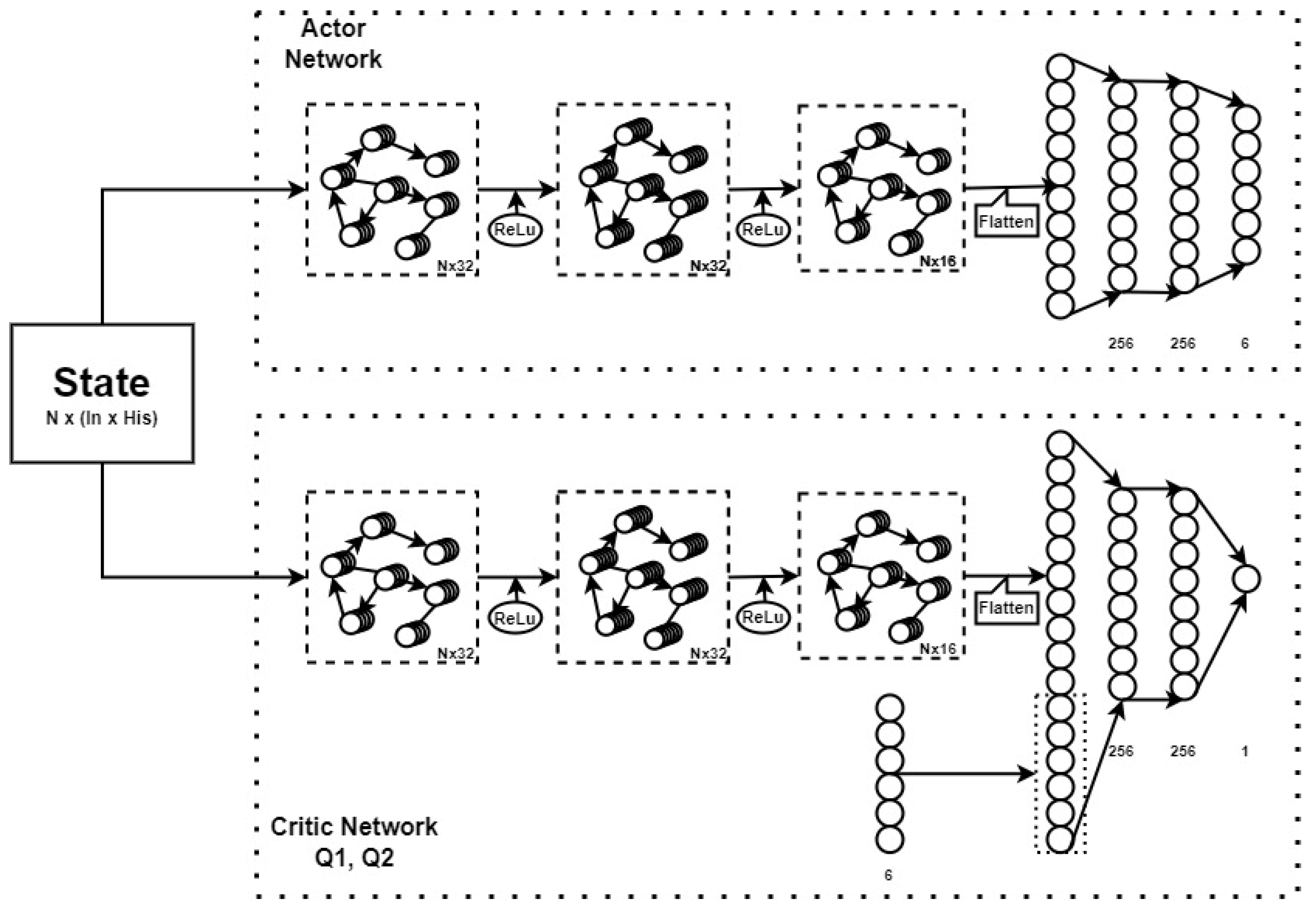
2. Network Architecture
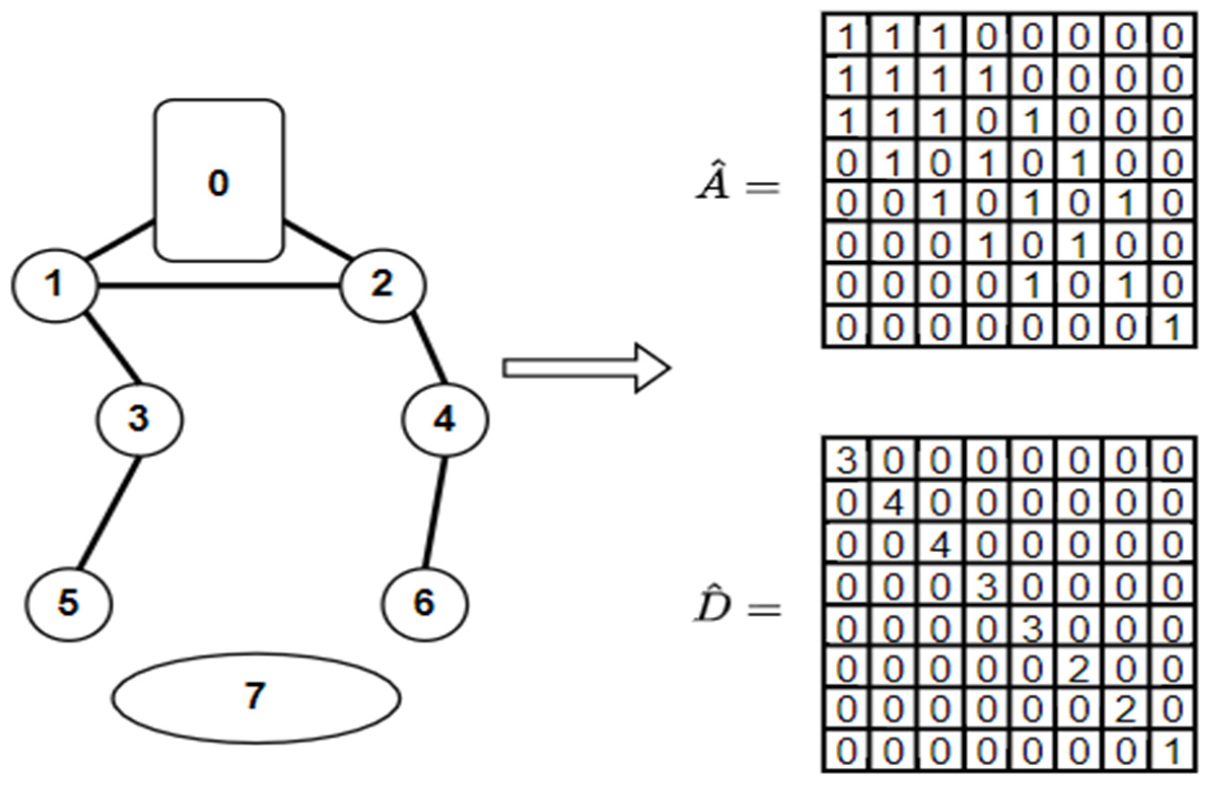
2.1. Graph Convolutional Network
2.2. Twin Delayed Deep Deterministic Policy Gradient
- The algorithm uses an actor network , two critic networks , corresponding to these three networks are their target networks: one target actor network and two target critic networks (i = 1, 2). Where and are the learning parameters of the actor and critic network, respectively, and similarly and are the parameters of the target actor network and the target critic networks;
- In order for the agent to explore a variety of states in the environment, actions computed from the actor network have a noise added [42]. This noise helps the data in replay buffer B to be augmented, and the noise in TD3 algorithms follows a Gaussian distribution [20]. Both the action “a” and the target action “a′” are added a noise , (with ). The Bellman equation [43] is used to calculate a target value as (9). In Equation (9), the smaller value between two outputs (,) of target critic networks is fed into the Bellman equation to avoid overestimating the Q-value:
- The parameter sets ( and ) are updated by minimizing the loss values (10) and (11) which are the expected value of the difference between the target value and the two Q-value, where (s, a, r, s’) are retrieved from replay buffer B:
2.3. GCTD3
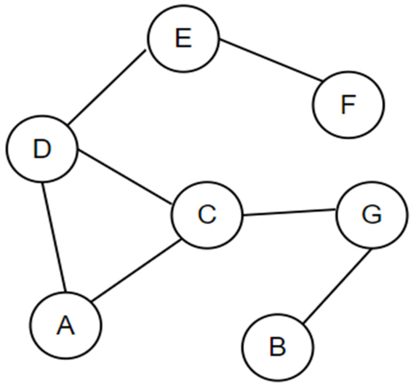
- The graph convolutional layers of our GCTD3 show efficiency with data in the form of the graph structure of the bipedal robot. The joints will learn each other’s relationships and constraints through these layers, the joints that are not connected will not affect each other. For example, the right knee joint and the right hip joint can share their attributes with each other, but the left knee joint and the right knee joint are not directly related;
- GCNs do not need to use a large number of weights to increase the joint features of the robot joints, so the computational volume is not too large even when using many previous states combined as the input of the neural network. According to Equation (7), the number of weights used for a joint to increase the number of its features from F to F’ is only equal to F × F’.
3. Training Process
3.1. Simulation Environment
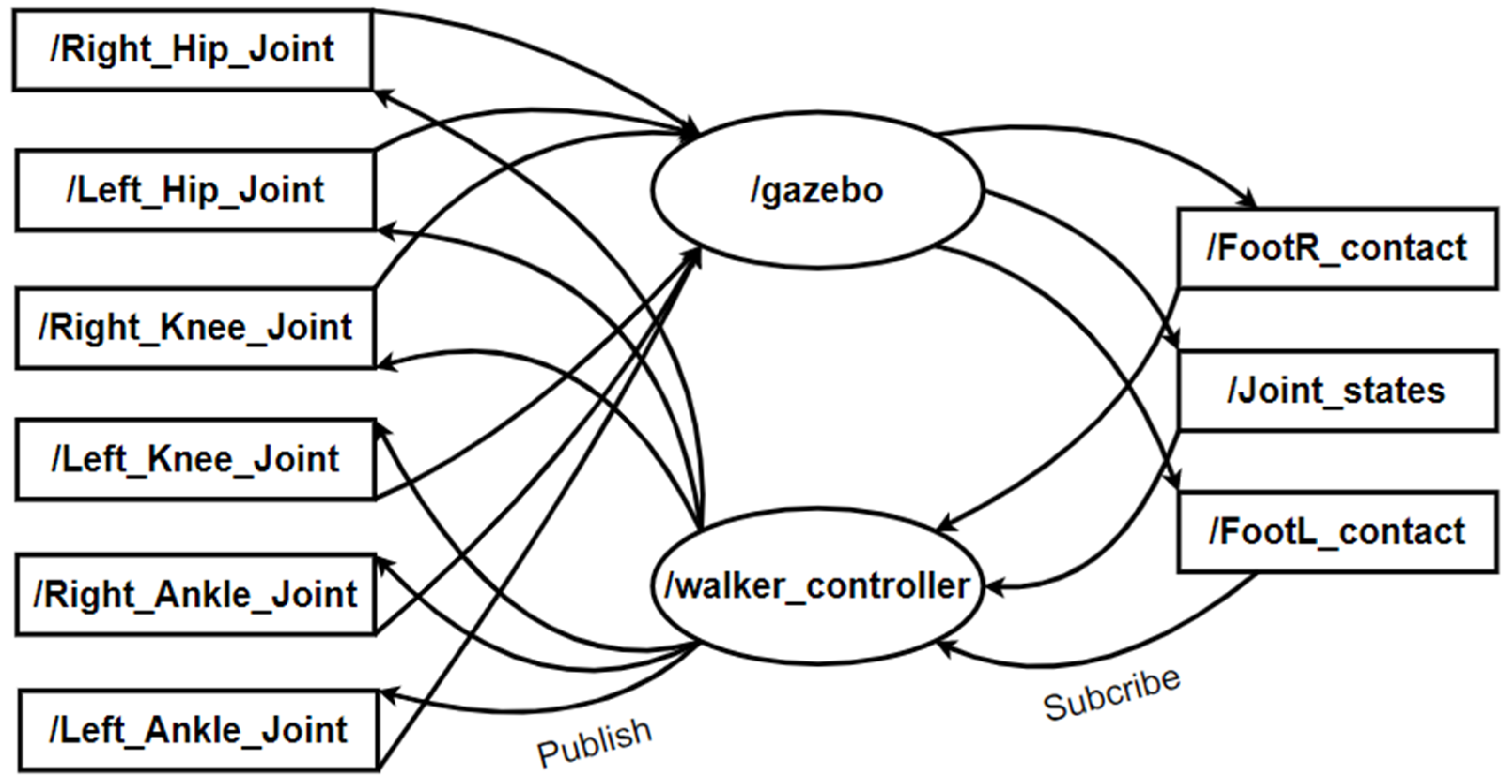
- Environment: Gazebo simulation environment receives control signals through the ROS with a frequency of 50 Hz, i.e., ROS will take the state from the environment and calculate the reward of that state to store data into a replay buffer every 0.02 s;
- State: At each joint of the robot model, sensors are placed to measure the information received from the environment for the agent to process. The sent signals contain information of the angular position and angular velocity of the joints, the coordinates of the robot’s body in the vertical direction and the robot’s speed according to the robot’s movement direction, and the signals from the sensor located at the feet to know whether the robot touches the ground or not, five consecutive states from t − 5 to t are concatenated again to form the input state of the neural network during training;
- Action: Before sending the robot control signals, the action corresponding to the desired angle coordinates of the joints is calculated by our proposed network, the action consists of six values corresponding to the desired angle of six joints: left hip joint, right hip joint, left knee joint, right knee joint, left ankle joint and right ankle joint. The angle ranges of these joints are limited as shown in Table 2;
- Reward: We use a dense reward function based on the actual human gait to make the algorithm easier to converge. While walking, the robot always has two states: one-foot contacts with the ground and two feet contact with the ground (Figure 7). In each state, the height of the body robot has different values. In the paper [25], only an average value of the body height during motion is used as a basis height for the robot to learn, two average values of the body height corresponding to two grounding states of the legs in motion are used in this paper. At the single phase of walking (Figure 7a,b), the average height of the robot’s body reaches a higher value than that at the double phase of walking (Figure 7c,d). In addition, the robot will also be punished if it performs actions that delay its movement such as falling or standstill, the details of the reward function are presented in Table 3.
3.2. Experiment
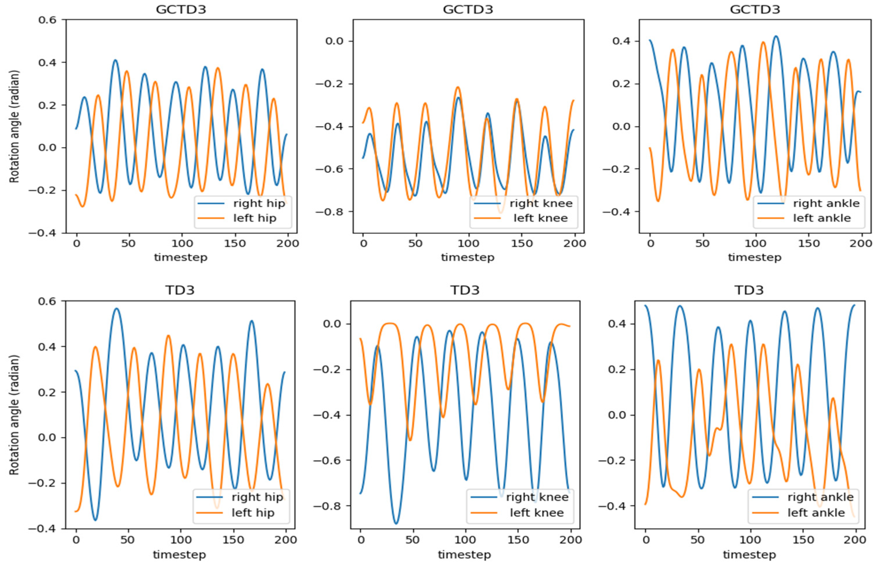
4. Evaluation
5. Conclusions
Supplementary Materials
Author Contributions
Funding
Institutional Review Board Statement
Informed Consent Statement
Data Availability Statement
Conflicts of Interest
References
- Kipf, T.N.; Welling, M. Semi-Supervised Classification with Graph Convolutional Networks. In Proceedings of the 5th International Conference on Learning Representations (ICLR 2017), Toulon, France, 24–26 April 2017. [Google Scholar]
- Defferrard, M.; Bresson, X.; Vandergheynst, P. Convolutional Neural Networks on Graphs with Fast Localized Spectral Filtering. In Proceedings of the 30th International Conference on Neural Information Processing Systems (NIPS’16), Barcelona, Spain, 4–9 December 2016; pp. 3844–3852. [Google Scholar]
- Kormushev, P.; Calinon, S.; Caldwell, D.G. Reinforcement Learning in Robotics: Applications and Real-World Challenges. Robotics 2013, 2, 122–148. [Google Scholar] [CrossRef] [Green Version]
- Kober, J.; Bagnell, J.A.; Peters, J. Reinforcement learning in robotics: A survey. Int. J. Robot. Res. 2013, 32, 1238–1274. [Google Scholar] [CrossRef] [Green Version]
- Zhu, H.; Yu, J.; Gupta, A.; Shah, D.; Hartikainen, K.; Singh, A.; Kumar, V.; Levine, S. The Ingredients of Real-World Robotic Reinforcement Learning. arXiv 2020, arXiv:2004.12570. [Google Scholar]
- Tuomas, H.; Sehoon, H.; Aurick, Z.; Jie, T.; George, T.; Sergey, L. Learning to Walk via Deep Reinforcement Learning. arXiv 2019, arXiv:1812.11103. [Google Scholar]
- Michael, B.; Fadri, F.; Tonci, N.; Roland, S.; Juan, I.N. Comparing Task Simplifications to Learn Closed-Loop Object Picking Using Deep Reinforcement Learning. IEEE Robot. Autom. Lett. 2019, 2, 1549–1556. [Google Scholar]
- Gu, S.; Holly, E.; Lillicrap, T.; Levine, S. Deep reinforcement learning for robotic manipulation with asynchronous off-policy updates. In Proceedings of the IEEE international conference on robotics and automation (ICRA), Singapore, 29 May–3 June 2017; pp. 3389–3396. [Google Scholar]
- Zhang, K.; Hou, Z.; Silva, C.W.; Yu, H.; Fu, C. Teach Biped Robots to Walk via Gait Principles and Reinforcement Learning with Adversarial Critics. arXiv 2019, arXiv:1910.10194. [Google Scholar]
- Peters, J.; Vijayakumar, S.; Schaal, S. Reinforcement learning for humanoid robotics. In Proceedings of the IEEE-RAS international conference on humanoid robots, Karlsruhe-Munich, Germany, 29–30 September 2003; pp. 1–20. [Google Scholar]
- Morimoto, J.; Cheng, G.; Atkeson, C.G.; Zeglin, G. A simple reinforcement learning algorithm for biped walking. In Proceedings of the IEEE International Conference on Robotics and Automation (ICRA ’04), New Orleans, LA, USA, 26 April–1 May 2004. [Google Scholar]
- Krishna, L.; Mishra, U.A.; Castillo, G.A.; Hereid, A.; Kolathaya, S. Learning Linear Policies for Robust Bipedal Locomotion on Terrains with Varying Slopes. In Proceedings of the IEEE/RSJ International Conference on Intelligent Robots and Systems (IROS), Prague, Czech Republic, 27 September–1 October 2021; pp. 5159–5164. [Google Scholar]
- Siekmann, J.; Valluri, S.S.; Dao, J.; Bermillo, L.; Duan, H.; Fern, A.; Hurst, J.W. Learning Memory-Based Control for Human-Scale Bipedal Locomotion. arXiv 2020, arXiv:2006.02402. [Google Scholar]
- Peng, X.B.; Berseth, G.; Yin, K.; Van De Panne, M. Deeploco: Dynamic locomotion skills using hierarchical deep reinforcement learning. ACM Trans. Graph. 2017, 36, 41. [Google Scholar] [CrossRef]
- Atique, M.U.; Sarker, R.I.; Ahad, A.R. Development of an 8DOF quadruped robot and implementation of Inverse Kinematics using Denavit–Hartenberg convention. Heliyon 2018, 4, e01053. [Google Scholar] [CrossRef] [PubMed] [Green Version]
- Gor, M.M.; Pathak, P.M.; Samantaray, A.K.; Yang, J.M.; Kwak, S.W. Jacobian based control of walking robot with compliant legs. In Proceedings of the 6th International Conference on Integrated Modeling and Analysis in Applied Control and Automation, Vienna, Austria, 19–21 September 2012; pp. 171–177. [Google Scholar]
- Farshidian, F.; Jelavic, E.; Winkler, A.W.; Buchli, J. Robust whole-body motion control of legged robots. In Proceedings of the IEEE/RSJ International Conference on Intelligent Robots and Systems (IROS), Vancouver, BC, Canada, 24–28 September 2017; pp. 4589–4596. [Google Scholar]
- Khoi, P.B.; Nguyen Xuan, H. Fuzzy Logic-Based Controller for Bipedal Robot. Appl. Sci. 2021, 11, 11945. [Google Scholar] [CrossRef]
- Konda, V.R.; Tsitsiklis, J.N. Actor-Critic Algorithms. In Proceedings of the Neural Information Processing Systems (NIPS); MIT Press: Cambridge, MA, USA, 29 November–4 December 1999; pp. 1008–1014.
- Fujimoto, S.; Van Hoof, H.; Meger, D. Addressing Function Approximation Error in Actor-Critic Methods. In Proceedings of the International Conference on Machine Learning Conference (ICML), Stockholm, Sweden, 10–15 July 2018; pp. 1587–1596. [Google Scholar]
- Tuomas, H.; Aurick, Z.; Pieter, A.; Sergey, L. Soft Actor-Critic: Off-Policy Maximum Entropy Deep Reinforcement Learning with a Stochastic Actor. In Proceedings of the International Conference on Machine Learning, Stockholm (ICML), Stockholm, Sweden, 10–15 July 2018; pp. 1861–1870. [Google Scholar]
- Lillicrap, T.P.; Hunt, J.J.; Pritzel, A.; Heess, N.; Erez, T.; Tassa, Y.; Silver, D.; Wierstra, D. Continuous control with deep reinforcement learning. In Proceedings of the 4th International Conference on Learning Representations (ICLR), San Juan, Puerto Rico, 2–4 May 2016. [Google Scholar]
- Mnih, V.; Badia, A.P.; Mirza, M.; Graves, A.; Lillicrap, T.P.; Harley, T.; Silver, D.; Kavukcuoglu, K. Asynchronous methods for deep reinforcement learning. In Proceedings of the International Conference on Machine Learning (ICML’16), New York, NY, USA, 19–24 June 2016; pp. 1928–1937. [Google Scholar]
- Kumar, A.; Paul, N.; Omkar, S. Bipedal Walking Robot using Deep Deterministic Policy Gradient. arXiv 2018, arXiv:1807.05924. [Google Scholar]
- Khoi, P.B.; Giang, N.T.; van Tan, H. Control and Simulation of a 6-DOF Biped Robot based on Twin Delayed Deep Deterministic Policy Gradient Algorithm. Indian J. Sci. Technol. 2021, 14, 2460–2471. [Google Scholar] [CrossRef]
- Connor, W.C.; Wengong, J.; Luke, R.; Timothy, F.J.; William, G.; Tommi, S.J.; Regina, B.; Klavs, F.J. A graph-convolutional neural network model for the prediction of chemical reactivity. Chem. Sci. J. 2019, 10, 370–377. [Google Scholar]
- Duvenaud, D.; Dougal, M.; Aguilera-Iparraguirre, J.; Gómez-Bombarelli, R.; Timothy, H.; Aspuru-Guzik, A.; Ryan, P.A. Convolutional Networks on Graphs for Learning Molecular Fingerprints. In Proceedings of the Advances in Neural Information Processing Systems 28 (NIPS 2015), Montreal, QC, Canada, 7–12 December 2015; pp. 2215–2223. [Google Scholar]
- Ying, R.; He, R.; Chen, K.; Eksombatchai, P.; Hamilton, W.L.; Leskovec, J. Graph convolutional neural networks for web-scale recommender systems. In Proceedings of the 24th ACM SIGKDD International Conference on Knowledge Discovery & Data Mining, London, UK, 19–23 August 2018; pp. 974–983. [Google Scholar]
- Yan, S.; Xiong, Y.; Lin, D. Spatial Temporal Graph Convolutional Networks for Skeleton-Based Action Recognition. arXiv 2018, arXiv:1801.07455. [Google Scholar]
- Tang, Y.; Tian, Y.; Lu, J.; Li, P.; Zhou, J. Deep progressive reinforcement learning for skeleton-based action recognition. In Proceedings of the IEEE Conference on Computer Vision and Pattern Recognition, Salt Lake City, UT, USA, 18–22 June 2018; pp. 5323–5332. [Google Scholar]
- Shi, L.; Zhang, Y.; Cheng, J.; Lu, H. Two-Stream Adaptive Graph Convolutional Networks for Skeleton-Based Action Recognition. In Proceedings of the IEEE/CVF Conference on Computer Vision and Pattern Recognition (CVPR), Long Beach, CA, USA, 16–20 June 2019. [Google Scholar]
- Shi, L.; Zhang, Y.; Cheng, J.; Lu, H. Skeleton-based action recognition with directed graph neural networks. In Proceedings of the IEEE/CVF Conference on Computer Vision and Pattern Recognition, Long Beach, CA, USA, 16–20 June 2019; pp. 7912–7921. [Google Scholar]
- Jiang, J.; Dun, C.; Lu, Z. Graph Convolutional Reinforcement Learning for Multi-Agent Cooperation. arXiv 2018, arXiv:1810.09202. [Google Scholar]
- Quigley, M.; Conley, K.; Gerkey, B.P.; Faust, J.; Foote, T.; Leibs, J.; Wheeler, R.; Ng, A.Y. ROS: An open-source Robot Operating System. In Proceedings of the ICRA Workshop on Open Source Software, Kobe, Japan, 12–17 May 2009. [Google Scholar]
- Quigley, M.; Gerkey, B.; Smart, W.D. Programming Robots with ROS: A Practical Introduction to the Robot Operating System; O’Reilly Media, Inc.: Newton, MS, USA, 2015. [Google Scholar]
- Cañas, J.M.; Perdices, E.; García-Pérez, L.; Fernández-Conde, J. A ROS-Based Open Tool for Intelligent Robotics Education. Appl. Sci. 2020, 10, 7419. [Google Scholar] [CrossRef]
- Koenig, N.; Howard, A. Design and use paradigms for Gazebo, an open-source multi-robot simulator. In Proceedings of the 2004 IEEE/RSJ International Conference on Intelligent Robots and Systems (IROS 2004), Sendai, Japan, 28 September–2 October 2004. [Google Scholar]
- Wenshuai, Z.; Jorge, P.Q.; Tomi, W. Sim-to-Real Transfer in Deep Reinforcement Learning for Robotics: A Survey 2020. In Proceedings of the IEEE Symposium Series on Computational Intelligence (SSCI), Canberra, Australia, 1–4 December 2020; pp. 737–744. [Google Scholar]
- Hammond, D.K.; Vandergheynst, P.; Gribonval, R. Wavelets on graphs via spectral graph theory. Appl. Comput. Harmon. Anal. 2011, 30, 129–150. [Google Scholar] [CrossRef] [Green Version]
- Richard, S.S.; Andrew, G.B. Reinforcement Learning: An Introduction, 2nd ed.; MIT Press: Cambridge, MA, USA, 2018. [Google Scholar]
- Kaelbling, L.P.; Littman, M.L.; Moore, A.W. Reinforcement learning: A survey. J. Artif. Intell. Res. 1996, 4, 237–285. [Google Scholar] [CrossRef] [Green Version]
- Rafael, S. Noise, Overestimation and Exploration in Deep Reinforcement Learning. Available online: https://arxiv.org/pdf/2006.14167v1.pdf (accessed on 28 January 2022).
- Bellman, R. Dynamic programing. Science 1966, 153, 34–37. [Google Scholar] [CrossRef] [PubMed]


| Link | Material | Mass (kg) | Height (m) |
|---|---|---|---|
| Body | Acrylonitrile butadiene styrene (ABS) | 4.0200 | 0.47 |
| Left Thigh | Acrylonitrile butadiene styrene (ABS) | 1.7324 | 0.267 |
| Right Thigh | Acrylonitrile butadiene styrene (ABS) | 1.7324 | 0.267 |
| Left Shank | Acrylonitrile butadiene styrene (ABS) | 0.7527 | 0.253 |
| Right Shank | Acrylonitrile butadiene styrene (ABS) | 0.7527 | 0.253 |
| Left Foot | Acrylonitrile butadiene styrene (ABS) | 0.4111 | 0.065 |
| Right Foot | Acrylonitrile butadiene styrene (ABS) | 0.4111 | 0.065 |
| Joint | Flexion (Rad) | Extension (Rad) | Annotation |
|---|---|---|---|
| Hip | 0.7854 | 0.7854 | α |
| Knee | 1.3962 | 0.0012 | β |
| Ankle | 0.7854 | 0.7854 | γ |
| Situation | Reward |
|---|---|
| Bonus | |
| Gait punishment | |
| Long ground contact time | |
| Fall down |
| Actor | Critics (Q1, Q2) | |
|---|---|---|
| Episode | 10,000 | |
| Policy update frequency | 2 | |
| Learning rate | 3 × 10⁻⁴ | 3 × 10⁻⁴ |
| Weight decay | 0.001 | 0.001 |
| Optimizer | Adam | Adam |
| Hidden GC layers | [32, 32, 16] | [32, 32, 16] |
| Hidden fully connected layers | [256, 256] | [256, 256] |
| Discount factor | 0.99 | 0.99 |
| DDPG | SAC | TD3 | GCTD3(our) | |
|---|---|---|---|---|
| Average reward | 241.28 ± 89.44 | 224.18 ± 56.96 | 370.31 ± 37.26 | 380.0 ± 18.47 |
| Position of the body robot (m) | −0.0114 | −0.0397 | −0.0020 | −0.0202 |
| Velocity (m/s) | 1.344 | 0.619 | 1.164 | 1.414 |
Publisher’s Note: MDPI stays neutral with regard to jurisdictional claims in published maps and institutional affiliations. |
© 2022 by the authors. Licensee MDPI, Basel, Switzerland. This article is an open access article distributed under the terms and conditions of the Creative Commons Attribution (CC BY) license (https://creativecommons.org/licenses/by/4.0/).
Share and Cite
Phan Bui, K.; Nguyen Truong, G.; Nguyen Ngoc, D. GCTD3: Modeling of Bipedal Locomotion by Combination of TD3 Algorithms and Graph Convolutional Network. Appl. Sci. 2022, 12, 2948. https://doi.org/10.3390/app12062948
Phan Bui K, Nguyen Truong G, Nguyen Ngoc D. GCTD3: Modeling of Bipedal Locomotion by Combination of TD3 Algorithms and Graph Convolutional Network. Applied Sciences. 2022; 12(6):2948. https://doi.org/10.3390/app12062948
Chicago/Turabian StylePhan Bui, Khoi, Giang Nguyen Truong, and Dat Nguyen Ngoc. 2022. "GCTD3: Modeling of Bipedal Locomotion by Combination of TD3 Algorithms and Graph Convolutional Network" Applied Sciences 12, no. 6: 2948. https://doi.org/10.3390/app12062948