1. Introduction
In recent years, the rapidly growing number of vehicles in urban transportation systems has raised huge challenges to society. Traffic congestion in the road network increases the commuting time of residents. In addition, it brings additional loss to the freight supply chain, which reduces the efficiency of economic activities and produces more pollution [
1]. To cope with these problems, constructing an efficient and convenient transportation system is of great necessity. Traffic prediction, which aims to predict future traffic states (e.g., traffic speed, traffic volume and traffic congestion index) in the road networks based on historical observations, acts a crucial part in the intelligent transportation system. Accurate prediction of traffic is the foundation of a wide range of real-world applications, such as travel time estimation, route planning, traffic light management, autonomous vehicle control and logistics distribution [
2].
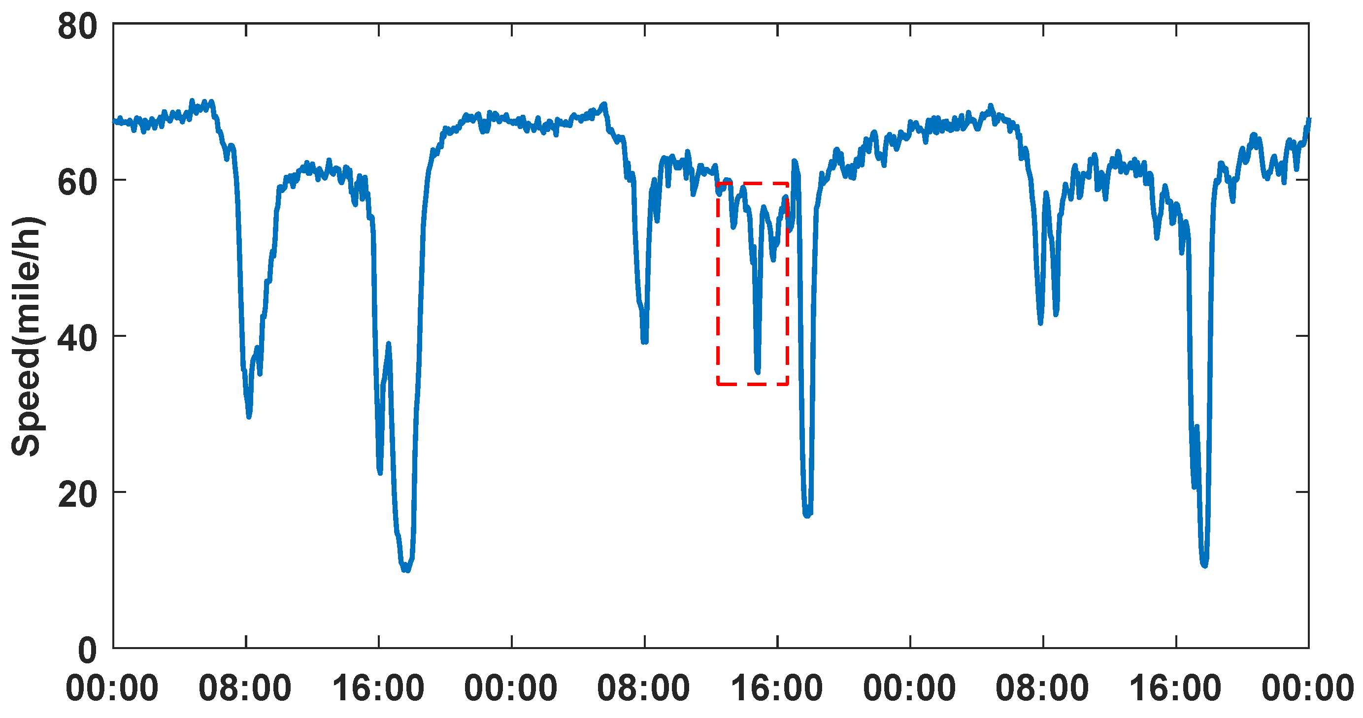
However, the tasks of traffic prediction remain challenging due to the complicated spatial and temporal dependency in the road networks. On the one hand, there are complex non-linear patterns in the time domain. The traffic conditions of a traffic node may follow a similar periodic trend over different days, but may see anomalous fluctuation in a short period. For example, as shown in
Figure 1, the traffic speed of a main road segment decreases during rush hours in the morning and evening, and increases back to a normal level gradually. However, as indicated by the red dotted box, there is a dramatic drop in the afternoon of a day, which increases the difficulty of making accurate prediction. On the other hand, traffic shows complicated spatial correlations. For example, as shown in
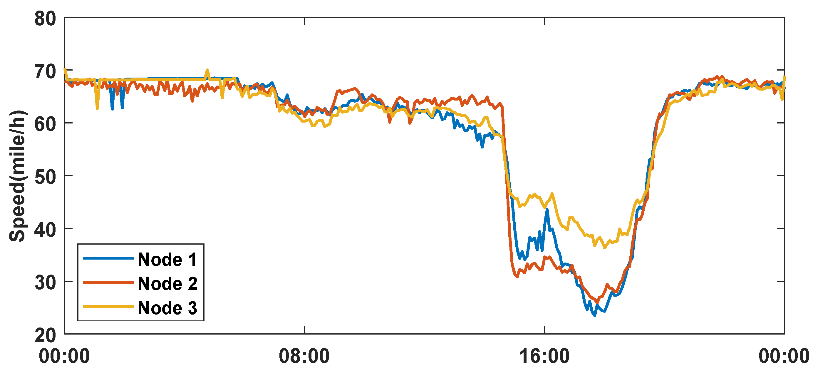
Figure 2, a traffic node usually has similar conditions to its neighboring nodes. The traffic speed of a road segment may become slower because of the congestion at its downstream road segment. Moreover, the traffic nodes that are not neighboring but with similar road topology or in similar functional areas tend to share similar patterns. Making accurate predictions requires comprehensive modeling of inter-node dependency. Therefore, with the spatiotemporal relations mentioned above, the tasks of traffic prediction are still challenging.
Extensive studies have been conducted on the tasks of traffic prediction. Early studies [
3,
4,
5] employ statistical methods or shallow machine-learning methods, which are limited in representation capability and thus have lower performance. With the emergence of deep learning, methods based on Recurrent Neural Networks (RNN) and Convolutional Neural Networks (CNN) are applied in traffic prediction to extract more complex spatial and temporal features [
6,
7,
8,
9,
10]. However, since CNNs can only process spatial traffic dependency in a grid-based manner, Graph Convolutional Networks (GCN) [
11] are introduced to handle traffic in irregular road networks with non-Euclidean structures. This kind of method aggregates information from selected neighbors according to a certain graph structure. More recently, integrating GCNs with other temporal models has become a paradigm for traffic-related tasks, which is followed by a number of studies [
12,
13,
14,
15,
16,
17].
Although existing approaches have achieved promising results, we find that the dynamics of spatial dependency have been rarely considered. Most of the existing graph-based works utilize one or more adjacency matrices to represent the connections among traffic nodes according to predefined similarity relations from different perspectives, such as road network distance [
12,
13], time-series similarity [
18], edge-wise line graph [
19] or point of interest (POI) similarity [
20]. Some works also use adaptive adjacency matrices with trainable parameters [
14,
21]. However, these inter-node relations are all static, which means that the spatial adjacency does not change along with time. Therefore, some implicit dynamic patterns of spatial adjacency may be neglected, limiting the performance of the spatiotemporal models.
In view of the limitations mentioned above, we aim to introduce dynamic representations into the adjacency graphs to achieve better prediction performance. In this paper, we propose a general traffic prediction framework named Time-Evolving Graph Convolutional Recurrent Network (TEGCRN), which takes advantage of time-evolving graph convolution to capture the dynamic inter-node dependency adaptively at different time slots. The contributions of our method can be summarized as follows:
We construct time-evolving adjacency graphs at different time slots with self-adaptive time embeddings and node embeddings based on a tensor-composing method. This method makes full use of information shared in the time domain and is parameter-efficient compared to defining an adaptive graph in each time slot.
To model the inter-node patterns in traffic networks, we apply a kind of mix-hop graph convolution that utilizes both the adaptive time-evolving graphs and a predefined distance-based graph. This kind of graph convolution module is verified as being effective in capturing more comprehensive inter-node dependency than those with static graphs.
We integrate the aforementioned graph convolution module with RNN encoder–decoder structure to form a general traffic prediction framework, which allows it to learn the dynamics of inter-node dependency when modeling traffic sequential features. Experiments on two real-world traffic datasets demonstrate the superiority of the proposed model over multiple competitive baselines, especially in short-term prediction.
The rest of the paper is organized as follows. In
Section 2, we review the related works systematically and explain their relations with our work. Then we formulate the problem and introduce the details of the proposed traffic prediction model in
Section 3. After that, we conduct experiments on real-world traffic datasets to evaluate the performance of the proposed method in
Section 4. In
Section 5 we conclude this paper.
3. Proposed Method
3.1. Problem Preliminaries
A traffic network can be regarded as a weighted directed graph . Here, is the set of N traffic nodes (i.e., sensors or road segments), is the set of edges (i.e., directed connections between traffic nodes), is a certain type of weighted adjacency matrix representing the proximity between each nodes pair, e.g., road distance graph.
The traffic features observed at time slot
t are represented as the graph signals
, where
F is the number of traffic features of each node. For example, the traffic features can be the traffic speed, traffic volume and congestion index of the road segments or other traffic related parameters. Given a traffic graph
, the purpose of traffic prediction is learning a model
f to map the historical graph signals observations of
P time steps to the signals of the next
Q time steps, which is denoted as:
3.2. Method Overview
Figure 3 illustrates the overview of our proposed method, which is referred to as Time-Evolving Graph Convolutional Recurrent Network (TEGCRN). The model mainly consists of three parts. First, the time-evolving adjacency graphs are generated through a tensor-composing method using the adaptive embeddings of traffic nodes and time slots. Then, the resulting adaptive graphs are combined with predefined static distance-based graphs and employed in graph convolution module to capture the inter-node information. Finally, the graph convolution modules with time-evolving graphs are used to replace the fully-connected layers in GRU to form an integrated RNN encoder–decoder predicting model. In each time step of the encoder–decoder, a different adaptive graph is selected depending on the time of day. The key thought of this method is to learn the implicit dynamics of spatial adjacency together with the traffic sequential features so as to capture more detailed spatiotemporal information. In the following subsections, we will describe each part in detail.
3.3. Generation of Time-Evolving Adaptive Graphs
As mentioned above, the spatial relationships among traffic nodes vary along with time, so our aim is to model these dynamics adaptively using time-evolving adjacency graphs. Moreover, we assume that the dynamics of the spatial adjacency also follow the periodicity in a day. Thus, the same time slot on different days can share a graph. Previous works [
14,
21] adopt matrix multiplication of trainable node embeddings to construct static adjacency graphs. The obtained adaptive graphs are evaluated to be effective in capturing global spatial information. To extend the adaptive graph to a time-evolving manner, a simple idea is to directly assign a distinct set of node-embedding parameters to each time slot. However, such a method may lead to a large number of trainable parameters, making it hard to converge, especially when the number of traffic nodes
N is large. To reduce the number of model parameters, we employ a tensor-composing method similar to [
32] to generate the time-evolving adjacency graphs.
Suppose that a day is divided into
time slots, and the traffic network contains
N traffic nodes. We first construct three embedding matrices
,
,
and a core tensor
, where
d is the embedding dimension,
. Specifically,
represents the embedding matrix of different time slots in a day,
represents the embedding matrix of source nodes,
represents the embedding matrix of target nodes. Tensor
builds connections among these embeddings and models the implicit factors shared across time and space. All these embeddings and the core tensor are trainable and randomly initialized. Next, a spatiotemoral tensor
is calculated as the following formula:
where
denotes the tensor mode-
i product [
33]. Specifically, the elements in
can be denoted as
Then, non-linear transformation and normalization are applied to
to obtain the tensor of time-evolving graphs
:
where the softmax normalization is operated in the last dimension. The
l-th slice of
along its first dimension
is the adaptive spatial adjacency graph of the
l-th time slot in a day.
With the approach above, we build connections between the representations of traffic nodes and the representations of time slots through the calculations of tensor composing. The resulting adaptive time-evolving graphs actually denote how much importance should be attached to different node pairs in different time slot of a day when aggregating spatial information in the road network. Later, these graphs will be used in the graph convolution module to extract detailed spatial information.
3.4. Graph Convolution Module
A graph convolution module is used to capture spatial patterns by aggregating information based on the adjacency graphs. In our proposed model, we conduct graph convolution with both the aforementioned adaptive time-evolving graphs and predefined distance-based static graph. In this way, the static graph captures local patterns, and the time-evolving graphs provide dynamic inter-node dependency from a global view as a complement.
Following [
12], we build a distance-based static graph
using thresholded Gaussian kernel [
34] as:
where
denotes the shortest directed distance from node
to node
in the road network,
denotes the standard deviation of these distances, and
is the threshold to control the sparsity of the graph.
As mentioned in the
Section 3.2, in our proposed model the graph convolution operations are integrated with an RNN structure. The recurrent manner in RNN inherently expands the depth of the model. In fact, GCNs may suffer from performance degradation due to the over-smoothing problem when the layers go deeper [
31]. It is also argued that the entanglement of information propagation and feature transformation in GCN may limit the model performance [
35]. By decoupling feature transformation with propagation and adding residual of input representation [
36], or combining the representations of multiple layers [
26], these problems can be relieved to some extent. Motivated by these ideas, we employ graph convolution operations in two steps: information propagation and weighted mix-hop operation, similar to the method in [
21]. First, for a certain type of adjacency graph, the node information is propagated according to the graph topology and the node representations of
K hops are generated. Denote the origin node representation as
, and the representation of the
k-th hop
is calculated as:
where
is a hyper-parameter to control the ratio of residual original information,
is the normalized form of the adjacency graph. Then, weighted mix-hop operation is employed to obtain
using the propagated representations of all hops as per the following formula:
where
,
is the learnable weighted transformation matrix.
For a time slot t, the corresponding index in a day is , graph convolution operations are applied using three graphs: the time-evolving graph in this time slot , the distance-based static graph and its transposed one . For and , asymmetric normalization is applied with and . The time-evolving graphs have been normalized during generation. We further aggregate the mix-hop representations of these three graphs to obtain the final output of the entire graph convolution module . For convenience, we briefly denote the calculations in this module as , where denotes the graph convolution operation, represents all the trainable parameters in a module. The static graph remains the same in all modules so we omit its notation in the formula.
3.5. Temporal Recurrent Module
RNN is devised as a recurrent structure which processes input signals and updates hidden states step-by-step. This kind of structure is suitable for combining with time-evolving graphs to model the dynamics of spatial dependency. As is shown in
Figure 3, in each time step, a different adaptive graph is selected according to the time index in a day. Then, following [
12,
19], we replace the matrix multiplication in GRU with the graph convolution module introduced in the previous subsection. The structure of the resulting recurrent unit is shown in
Figure 4, which is referred to as Time-evolving Graph Convolutional GRU (TGCGRU).
For each time slot
t, given the corresponding time-evolving graph
, the calculations in TGCGRU are fomulated as follows:
where
,
denote the input traffic features and output hidden state at time step
t, respectively,
h is the hidden size of TGCGRU. The notation ‖ denotes concatenation operation,
is the sigmoid function, and ⊙ denotes the Hadamard product.
and
represent the reset gate and update gate, respectively.
,
,
are parameters for the corresponding graph convolution modules and
,
,
are trainable bias vectors. These parameters share all the time steps.
We stack multiple TGCGRUs to form an RNN sequence-to-sequence architecture [
37] for multi-step traffic prediction, as is shown at the top of
Figure 3. On the decoder side, an additional fully-connected layer is used to map the output hidden state of TGCGRU to the output features. The output features of all time steps in the decoder are the predictions we need. Both the embedding parameters for time-evolving graph generation and the parameters in TGCGRU are trained together in an end-to-end manner. To relieve the discrepancy in input distribution between the training and testing stage, the scheduled sampling [
38] strategy is applied. During training, the decoder takes as input either the ground truth with probability
or the prediction of the previous step with probability
. The probability of the
i-th iteration
is calculated as
where
is a constant to control the speed of probability decay.
3.6. Example of the Prediction Process of TEGCRN
In this section, we will explain the entire process of TEGCRN and take the prediction for traffic speed as an example. Given the historical speed observations of
P steps
, the prediction targets are the speeds of the next
Q steps. In this case,
represents the speed of all the
N nodes at time slot
t and
. As shown in
Figure 3, we first employ Equations (
2) and (
4) to generate tensor
and obtain the time-evolving graphs of the corresponding time slots
and
for the encoder and decoder, respectively. Next, for each historical time slot, the speed snapshot
and the corresponding time-evolving graph
are input to the TGCGRU encoder step-by-step, as the calculations show in Equation (
8). The graph convolution operations in Equation (
8) are formulated by Equations (
6) and (
7). The output in the last step of the encoder is used to initialize the hidden state of the decoder. Then, following the calculations similar to the encoder, in each step, the decoder takes the prediction of the previous step as input and generates the speed predictions
step-by-step.
4. Experiments and Discussion
4.1. Datasets
We evaluate the proposed model TEGRCN on two public real-world traffic datasets, METR-LA and PEMS-BAY, which were released by Li et al. in [
12]. METR-LA records the traffic speed data collected from 207 sensors on the highways of Los Angeles County, ranging from 1 March 2012 to 30 June 2012. PEMS-BAY records the speed data collected from 325 sensors in the bay area by California Transportation Agencies, ranging from 1 January 2017 to 30 June 2017. The units of the speed data are both miles per hour. Some basic statistics of these two datasets are listed in
Table 2. Each sensor in the road network is viewed as a traffic node. The numbers of the edges are counted according to the distance-based static adjacency graphs. We can see that there is a relatively high proportion of missing values in METR-LA while the counterpart in PEMS-BAY is almost negligible. Following the data pre-processing procedures in [
12], we set the interval between two time steps to 5 min. Then, each dataset is split in chronological order, with 70% for training, 10% for validation and 20% for testing. Z-score normalization is applied to the inputs.
In these two datasets, only the traffic speed in the road network is provided, so the number of traffic features is . Take METR-LA as an example, the graph of traffic network contains nodes, so the traffic features (also called as graph signals) at a specific time slot t can be denoted as . To make multiple-steps-ahead predictions with the historical observations, the series of these traffic features are input to the encoder–decoder of the proposed model step-by-step.
4.2. Baseline Methods
To verify the predicting performance of TEGCRN, we compare it with typical time-series models and some representative graph-based spatiotemporal networks. The selected baselines are introduced as follows:
HA: Historical Average, which views the traffic flow as seasonal signals and predicts future speed with the average of the values at the same time slots of previous weeks.
ARIMA: Auto-Regressive Integrated Moving Average model with Kalman filter, a traditional time-series predicting method.
FC-LSTM [
37]: RNN sequence-to-sequence model with LSTM units, using a fully-connected layer when calculating the inner hidden vectors.
DCRNN [
12]: Diffusion Convolutional Recurrent Neural Network, which combines the bidirectional graph convolution with GRU encoder–decoder model. Only the distance-based graph is utilized and the adjacency in different time steps remains static.
STGCN [
13]: Spatiotemporal Graph Convolutional Network, which alternately stacks temporal 1-D CNN with spectral graph convolution ChebyNet to form a predicting framework in a complete convolutional manner. Likewise, it relies only on the distance-based static graph.
Graph-WaveNet [
14]: Based on the alternate convolutional architecture in [
13], this model applies dilated convolution in the time dimension and incorporates an adaptive adjacency graph in the graph convolution module.
MTGNN [
21]: This model introduces a uni-directional adaptive graph and mix-hop propagation into graph convolutions, and introduces dilated inception layers on the time dimension to capture features in receptive fields of multiple sizes.
4.3. Experiments Settings and Metrics
As described in
Section 3, the proposed model aims to make a multi-step prediction of future traffic states according to historical observations. Following the typical settings in the baseline methods using the same datasets, we set both the length of historical observations and future predictions to one hour, i.e.,
, to make fair comparison. When generating the time-evolving graphs, the embedding dimension
d is set to 30 for METR-LA and 40 for PEMS-BAY. Since the length of each time slot is 5 min, the number of time slots in a day
. As for the graph convolution module, the maximum hop of
K is set to 2 for both datasets and
is set to 0.01. The number of TGCGRU layers is set to two and the size of the hidden state in TGCGRU is set to 40 for METR-LA and 50 for PEMS-BAY. These hyper-parameters that are related to the proposed model are all selected via grid search. During the training process, the value
for scheduled sampling is set to 2000. The model is trained by Adam optimizer and the learning rate is initialized to 0.01 with a decay rate of 0.1. Mean absolute error (MAE) is selected as the loss function. The batch size of input data is set to 64 for METR-LA and 32 for PEMS-BAY. Early stopping strategy is employed. For each dataset, the experiment is repeated five times to obtain the average metrics. To evaluate the performance of traffic prediction, three types of metrics are used, including mean absolute error (MAE), root-mean-squared error (RMSE) and mean absolute percentage error (MAPE).
4.4. Prediction Performance
The prediction results of our proposed method TEGCRN and the baseline methods on METR-LA and PEMS-BAY are shown in
Table 3 and
Table 4, respectively. We report the results for 15 min (3 steps)-, 30 min (6 steps)-, 60 min (12 steps)-ahead predictions to show the performance in the short term, middle term and long term.
As shown in
Table 3 and
Table 4, TEGCRN achieves higher performance on both datasets. It almost outperforms these baseline methods in all the time steps except for the long-term prediction on METR-LA. We can also see that the performances of GCN-based methods significantly outperform traditional series models such as ARIMA and FC-LSTM. This emphasizes the importance of introducing spatial information into traffic prediction. In contrast to the models using only predefined distance-based graphs such as DCRNN and STGCN, Graph-WaveNet and MTGNN achieve better performance. This is because more inter-node dependency can be learned by the inner adaptive adjacency graph from a global view. Moreover, the inception layers in MTGNN may capture more temporal patterns in different time scales, which helps MTGNN surpass Graph-WaveNet in long-term prediction. By using time-evolving graph convolutions and integrating them with recurrent structure, our proposed model TEGCRN can capture more implicit dynamics of inter-node dependency, so it can achieve better performance compared with the models with static graphs. Since the recurrent structure in RNN usually suffers from accumulative errors when the number of output time steps increases, TEGCRN may be more sensitive to missing values in input data than the CNN-based models. However, the proportion of missing values of METR-LA is much higher than that of PEMS-BAY. This may lead to the small performance margin between TEGCRN and MTGNN when making long-term predictions on METR-LA. To sum up, our proposed model TEGCRN shows its superiority over multiple competitive traffic-predicting baseline models especially in short-term prediction.
4.5. Ablation Study
We conduct an ablation study on the METR-LA dataset to validate the effectiveness of the graph convolution module with adaptive time-evolving graphs. We first build a model that replaces the time-evolving graphs in TEGCRN with a static adaptive graph as the manner in [
14]. Additionally, we further remove the time-evolving graph generation module and use only static predefined distance-based graph, as per the manner in [
12]. For these models, we calculate the average metrics of all the output time steps. The results are reported in
Table 5. We can see that, with learned global dependencies, the convolution with adaptive graph achieves higher performance than that with only predefined distance-based graph. Furthermore, the proposed time-evolving graph convolution in TEGCRN further improves the prediction performance by capturing more implicit inter-node dynamics.
Figure 5 shows the heatmaps of the normalized distance-based static adjacency graph and the learned time-evolving adjacency graphs in some selected time slots. A darker color means a higher value of weight between the corresponding nodes. When the static graph assigns high weights to the neighboring node pairs in a local manner, the time-evolving graphs can learn some other sparse connections among the nodes from a global view. In different time slots, the trained time-evolving graphs attach different importance to the traffic node pairs and form dynamic topologies. These learned implicit dynamics of inter-node dependency can act as the complement of the static distance-based graph. This helps the graph convolution to capture more urban semantics, which contributes to the better prediction performance. In sum, the proposed graph convolution with adaptive time-evolving graphs is effective to model more comprehensive inter-node dependencies than those with only static graphs.
4.6. Parameters Study
We studied the model performance with different values of two important hyper-parameters: the embedding dimension
d in the time-evolving graph generation module and the hidden size
h of GRU units. The latter is also the output dimension of the graph convolution module. For each experiment, we only change the selected hyper-parameter while fixing other settings. The average MAE loss of different settings on METR-LA and PEMS-BAY are shown in
Figure 6 and
Figure 7, respectively. The optimal values of both embedding dimension and hidden size on PEMS-BAY are larger because of the larger amount of traffic nodes. For METR-LA, we set the embedding dimension at 30 and the hidden size at 40. The counterparts of PEMS-BAY are 40 and 50. The performance on METR-LA is more sensitive to the values of hyper-parameters.
4.7. Discussion
The proposed model TEGCRN may need more costs when training the time-evolving adjacency graphs. However, once the model is trained and the weights in the time-evolving graphs are frozen, the time-evolving graphs can be stored offline and the calculations of graph generation are no longer needed. So, the computational complexity of the graph convolution modules is the same as those with static graphs when making predictions. In the experiments described in the previous subsections, we take the prediction task for the traffic speed as an example and set the number of traffic features . However, it is worth mentioning that the proposed model is devised as a general traffic prediction framework which can be applied to the predictions of other parameters in the traffic network (e.g., traffic volume and congestion index) and take multiple features as input. Therefore, the proposed model can be employed as a building block in different traffic support systems and provide more accurate predictions for multiple applications such as route planning and logistics distribution.


