1. Introduction
Selective laser melting (SLM) is an additive manufacturing (AM) process in which a 3D structure is constructed by successively melting material powder layers. The SLM process uses a high-energy laser beam to melt the powder, making it accessible to different materials, including metals. This technique can help to construct lighter, more complex geometries that are more robust, without any significant material wastage. Due to such advantages, SLM technology has increased in popularity and has made its way into large manufacturing industries such as aerospace, medical implants, automobiles, etc. [
1]. However, many challenges are associated with SLM products, including dimensional accuracy, part distortion, premature process termination, and mechanical properties, thus requiring further research and analysis [
1,
2].
Additive manufacturing (AM) efficiency and accuracy can be improved by using suitable material and process parameters. Broadly, the properties of a material, the process, and the environment define a large number of the parameters which affect the final product [
3], including laser speed, layer thickness, chamber temperature, etc. Therefore, it is important to understand each parameter’s impact on the AM process; there could also be possible interactions between the parameters. To meet specific design requirements in the AM, these material parameters and the process parameters may need to be optimized. SLM is a multiphysics process that occurs over different time and length scales [
4]. Among the major physical phenomena that occur during the process are radiation, convection phase change, absorption and phase change, etc. [
5]. Our understanding of the SLM process can be improved by using the design of experimental methods [
5]. However, experimenting on a large scale is time-consuming and costly. Such challenges can be addressed using a realistic numerical model of the process. A numerical model can help us generate a large number of data sets at a significantly lower cost than traditional experimental methods. However, SLM involves complex multiphysics and multiscale phenomena [
4] with many uncertainties, from the material powder bed to the melting and solidification processes. These uncertainties come from an insufficient understanding of the process, measurement error, scaling error, sampling error, and lack of information about the material properties [
6]. All these elements contribute to the model’s confidence level, which may limit SLM applications.
To increase the SLM product quality and production, we need to understand the sources of uncertainties; how they grow, and how they affect the final product quality. Two methods can be considered to tackle these issues and to increase trust in the SLM numerical model [
7] or the process: (1) uncertainty analysis (UA), and (2) sensitivity analysis (SA). Uncertainty analysis aids in understanding the uncertainty in model outputs due to the uncertainties in the model inputs; whereas, sensitivity analysis gives insight into how uncertainties in the model inputs and outputs are related to each other. Most of the reported UA and SA methods in AM are experiment-based, which leads to a high material wastage and makes the process expensive [
6]. In another approach, numerical models can be used to quantify the uncertainties in the SLM process. However, a full-scale (such as a finite elements-based) model could be computationally expensive and may take hours or days to complete depending on the simulation type. In addition, numerical models are deterministic, and usually do not consider the input variables’ uncertainties [
8].
This paper provides a framework to optimize the SLM process and study uncertainty and sensitivity analyses using a data-driven approach along with a 3D finite element model. As the discretization of SLM problems requires fine spatial meshes and a high number of time steps, the overwhelming demand for computational resources makes high-fidelity simulations too expensive computationally in the contexts of uncertainty propagation or inverse analysis studies. To alleviate this difficulty, we advocate the use of the data-driven approach, which consists of two major stages: (1) A database of high-fidelity solutions computed for a certain number of samples of the input data in the offline stage, which allows a surrogate model to be obtained using a regression method on a reduced basis; (2) Predictions on new data performed on the online stage using the surrogate model.
It is possible to a priori prescribe a reduced basis such as in the well-known polynomial chaos expansion (PCE), or to use neural networks for which the reduced basis is obtained adaptively. The data-driven approach does not require any modification of the high-fidelity source codes; these are used as a black box. However, the solutions database should be computed in a reasonable timeframe, for which parallel computing is deemed essential. We used PCE and neural network methods to build an efficient machine learning model. Genetic and evolutionary optimization algorithms were then used to find the optimal parameters. These models were validated on a benchmark SLM test [
9] for which the high-fidelity solutions were obtained using Ansys additive software.
After this introduction, the second section contains a brief literature survey on the problem.
Section 3 gives an overview of the mathematical methods used for statistical analysis, surrogate modeling, and optimization. The results of the benchmark test are discussed in
Section 4. Finally, concluding remarks are given in
Section 5.
2. Literature Review
Uncertainty sources can be classified into two categories: epistemic and aleatory uncertainty. Aleatory uncertainty in a system occurs due to natural causes such as fluctuation in the laser power, etc. The sources of epistemic uncertainty, meanwhile, are an incomplete understanding or a lack of knowledge, which can be further divided into two types, data uncertainty and model uncertainty. Data uncertainty arises because of improper measurements and an insufficient amount of measured data. Model uncertainty is used to quantify the difference between experimental data and numerical simulation models. For example, model uncertainty may occur due to the assumptions made to simplify the numerical model [
6]. To understand the relationship between uncertainties in input and output parameters, we proposed performing a sensitivity analysis (SA). These can be divided into two types, local and global sensitivity analyses. Local sensitivity analysis is derivative-based; this technique analyzes the effect of one parameter on the process by keeping other parameters constant. In global sensitivity analysis, all the input parameters are varied simultaneously, and the sensitivity is calculated over the whole sample space of each input.
There are different approaches to performing sensitivity and uncertainty analysis in SLM. The most popular method is trial and error experimentation. Delgado et al. [
10] conducted an experimental investigation to determine the influences of input parameters (laser speed, build direction, and layer thickness) on SLM output. They used a full factorial experimental design technique with three factors, and two levels for each factor. The dimensional accuracy, roughness, and mechanical properties were considered to measure the effect of input parameters. UA and SA of the AM process using experiments may give good results to some extent, but these analyses have various disadvantages. For example, experiments on a large scale lead to material wastage and a delay in final product delivery, subsequently increasing the product and process cost. Additionally, one component’s results may not be applicable for other SLM products, as results may vary with the problems [
6]. However, these issues can be addressed by using an efficient numerical simulation model.
Criales et al. [
11] used finite element modeling to analyze 2D temperature profiles and melt pool geometry. They performed a sensitivity analysis by changing one input parameter at a time while keeping the other parameters constant, and found that the powder reflectivity affects the melt pool geometry the most. However, changing parameters one at a time does not always provide good results, as this process fails to consider the interaction of parameters. Bruna-Rosso et al. [
12] conducted a global sensitivity analysis for SLM using a 2D numerical simulation model. They used 26 input parameters and calculated their influence on melt pool width, length, and maximum temperature. The effect on the output was calculated by simultaneously changing the input parameters instead of changing one at a time. They used the elementary effect technique and found that 16 of the parameters did not significantly affect the process output. Similarly, Lopez et al. [
13] used a numerical model for single-track simulation to identify uncertainties in the SLM process.
A 3D and more complex model for a single-track SLM was used by Ma et al. [
14] to identify the critical variable. They used a design of experiment (DOE) technique with a two-level screening system to separate the vital parameters. As the numerical simulation becomes more complex, the computation cost of the simulation will also increase. To make the numerical simulation more efficient, Kamath et al. [
15] proposed a framework to combine the numerical and experimental approaches to find critical parameters. They initially found the essential parameters and then used them to devolve a surrogate model for the melt pool. The developed surrogate model was then used to find the uncertainties in the system. A surrogate model provides an alternative and more efficient way to perform uncertainty and optimization analysis.
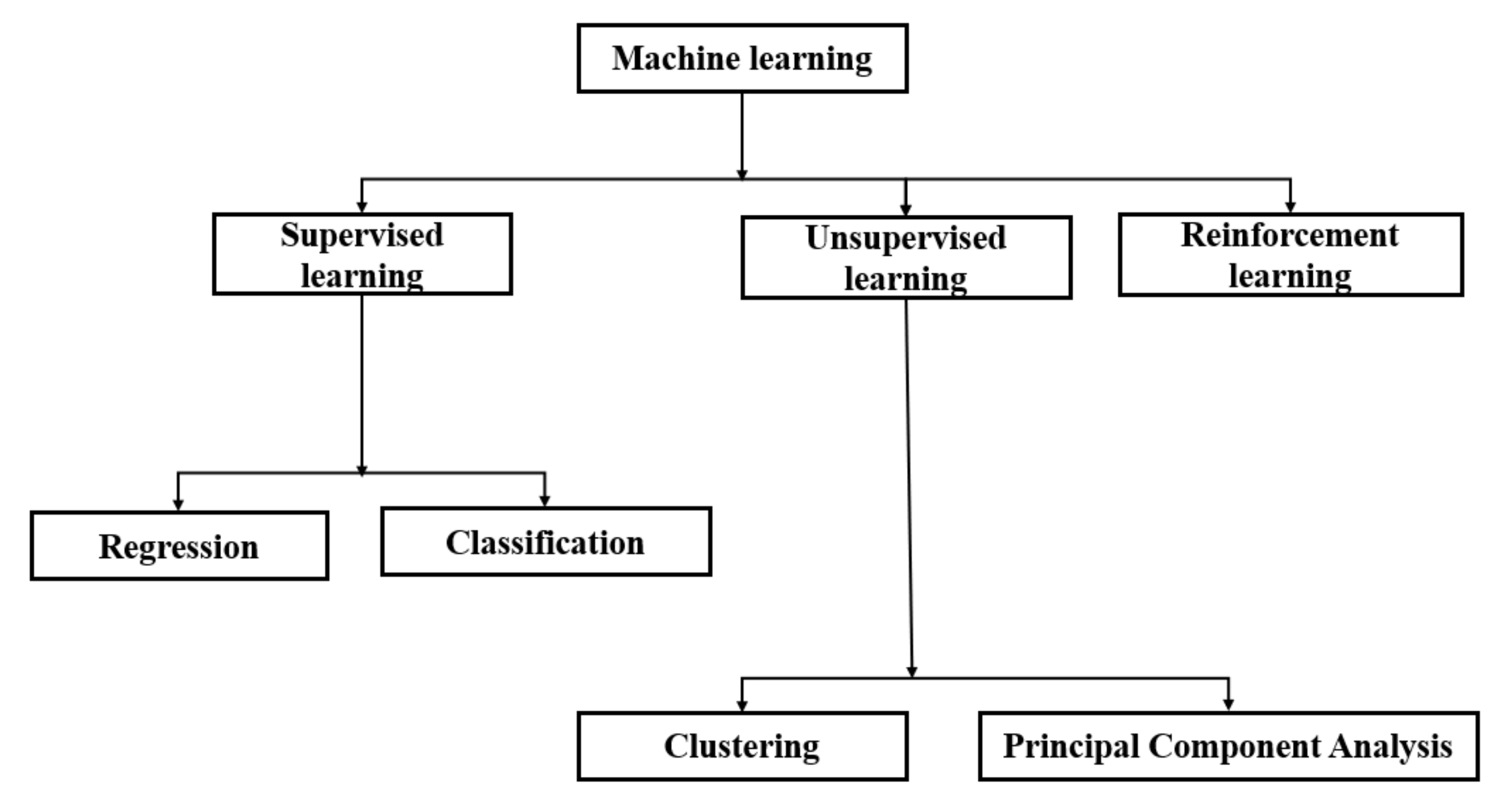
Surrogate modeling of the AM process using machine learning (ML) methods is still in its early stage. ML models can be classified into three types: (1) supervised learning, (2) unsupervised learning, and (3) reinforcement learning. In supervised learning, each input parameter space is labeled with an output, whereas in unsupervised learning, the input parameters do not have an output [
16]. On the other hand, reinforcement learning maximizes the reward signals by continuously learning the relation between the situation and the actions. The best example is self-driving cars. Different types of ML models have been used for AM analysis, as shown in
Figure 1. For example, a regression approach has been used to predict the AM part quality of parameter optimization, whereas the classification approach can detect defects, quality assessment or prediction, etc. [
16,
17]. Ravichander et al. [
18] presented a prediction model for SLM using an ANN method. The ANN model was trained with experimental results and was used to predict the SLM outputs on a set of different parameters. The primary input parameters were the laser power, hatch spacing, and scanning speed. In similar studies [
19,
20], an ANN model was used to construct a surrogate map between the laser parameters and outputs such as temperature, strains, etc., for an AM build part.
Recently, surrogate models have gained popularity for UA in the AM process. The most commonly used surrogate models in AM are support vector machines (SVM), neural networks (NNs), Gaussian process (GA) models, and polynomial chaos expansion [
6]. Cai and Mahadevan [
21] developed a methodology to study the uncertainty in a final product’s microstructure via the construction process parameters and environmental changes. They replaced the finite element model with the Gaussian surrogate model and applied it to study the relationship between the cooling rate and the final product’s microstructure. A similar methodology was adopted by Sankararaman [
22], who used a surrogate model to quantify the uncertainties in fatigue crack growth in AM. Tapia et al. [
23] proposed a Gaussian process-based surrogate model to make a response surface between the SLM process output and the input parameters. Their surrogate model was constructed using 96-single-track experimental data to predict the melt pool depth. The model was then used to calculate the melt pool depth at unobserved input process parameters.
Highly efficient machine learning models have provided an alternative framework for optimizing the AM process [
17]. Rong-ji et al. [
24] used an NN framework to optimize the selective laser sintering process’ parameters by minimizing the shrinkage. They trained the NN with experimental data, and then combined it with the genetic algorithm (GA) to find the input parameters’ optimal values. The proposed structure can be used to optimize any nonlinear and multitudinous system. Tapia et al. [
25] used this approach to predict the porosity of an SLM-built part using a Gaussian process-based model. Additionally, they provided a Bayesian framework to estimate the statistical model’s parameters, and then used the Kriging method to predict the given parameter settings’ porosity. This study’s primary disadvantage was that they only two parameters were used as input variables, whereas the SLM can be affected by many factors, including the materials and environment.
NNs and GAs are the most widely used methods for the optimization, modeling, and prediction of process parameters. Some of the popular GA methods used in AM are multi-gene genetic programming (MGGP), the multi-objective particle swarm optimizer (MOPSO), the non-dominated genetic algorithm, etc. [
26]. Padhye et al. [
27] used the MOPSO and the non-dominated sorting genetic algorithm (NSGA-II) to minimize the surface roughness and built time in the selective laser sintering (SLS) process.
The surface roughness and the built time are functions of the “build direction”, and so minimizing them aids in finding the optimal build orientation. A study by Padhye et al. also found that the NSGA-II outperforms the MOPSO in finding optimal results. In a similar study by Singhal et al. [
28], a conventional optimization algorithm based on a trust region method was used to optimize the stereolithography (SL) and the SLS process. The objective of Singhal et al.’s study was to increase the quality of the built surface and the support structure by determining the optimum deposition orientation for a building part.
3. Mathematical Model
A global sensitivity analysis considers the uncertainty in the input parameters and their influence on the uncertainty of the process output to rank the importance of each input parameter [
12]. In this paper, we have used a variance-based global sensitivity analysis (GSA), which is commonly used to quantify the sensitivity of output to input parameters. The basic concept behind the variance-based method is to decompose the output variance among each model input. To explain the variance-based GSA, let us consider the following model:
where
Y is the system output and
represents the independent input variables, which can be defined by a known probability distribution. If we compare this equation with our case, then
can be seen as the strain value, and the inputs are the machine properties, such as laser speed and layer thickness, etc. To calculate the effect of input parameters
on the variance of
, we assume that the actual value of
is
. The following conditional variance gives the change in the variance of
:
In the above Equation,
represents the conditional variance over the (p-1) input parameter space, including all the input parameters except
. As the exact value of
is unknown, we will take an average over all the potential values of
, which is given by:
The smaller value of
represents the greater importance of
in the variance of
. If we use the law of total variance, then we can write:
After a normalization, Equation (4) can be written as:
represents the first-order sensitivity index for the parameter
. The remaining terms in Equation (5) will help in calculating the total order index. Equation (1) is further decomposed into increasing orders of dimension, as:
In the above equation, if we assume that all the input factors are mutually independent, then there exists a simple decomposition where all the terms will be mutually orthogonal, and so the variance of the output (
) can be written as follows:
where
,
, …,
represents the variance of
,
, …,
, respectively. The first-order sensitivity index shown in Equation (6) can be obtained by using the first p term of the above decomposition.
Using a similar approach, we can find the higher order of sensitivity indices, such as the second-order indexes or the other higher indices.
3.1. Surrogate Modeling
A surrogate model is a mathematical representation of the relationship between the input and output parameters; it provides approximate outputs for new input values without explicitly solving the process. In the present study, we have used a deep neural network and polynomial chaos expansion to build our surrogate models.
3.1.1. Deep Neural Networks
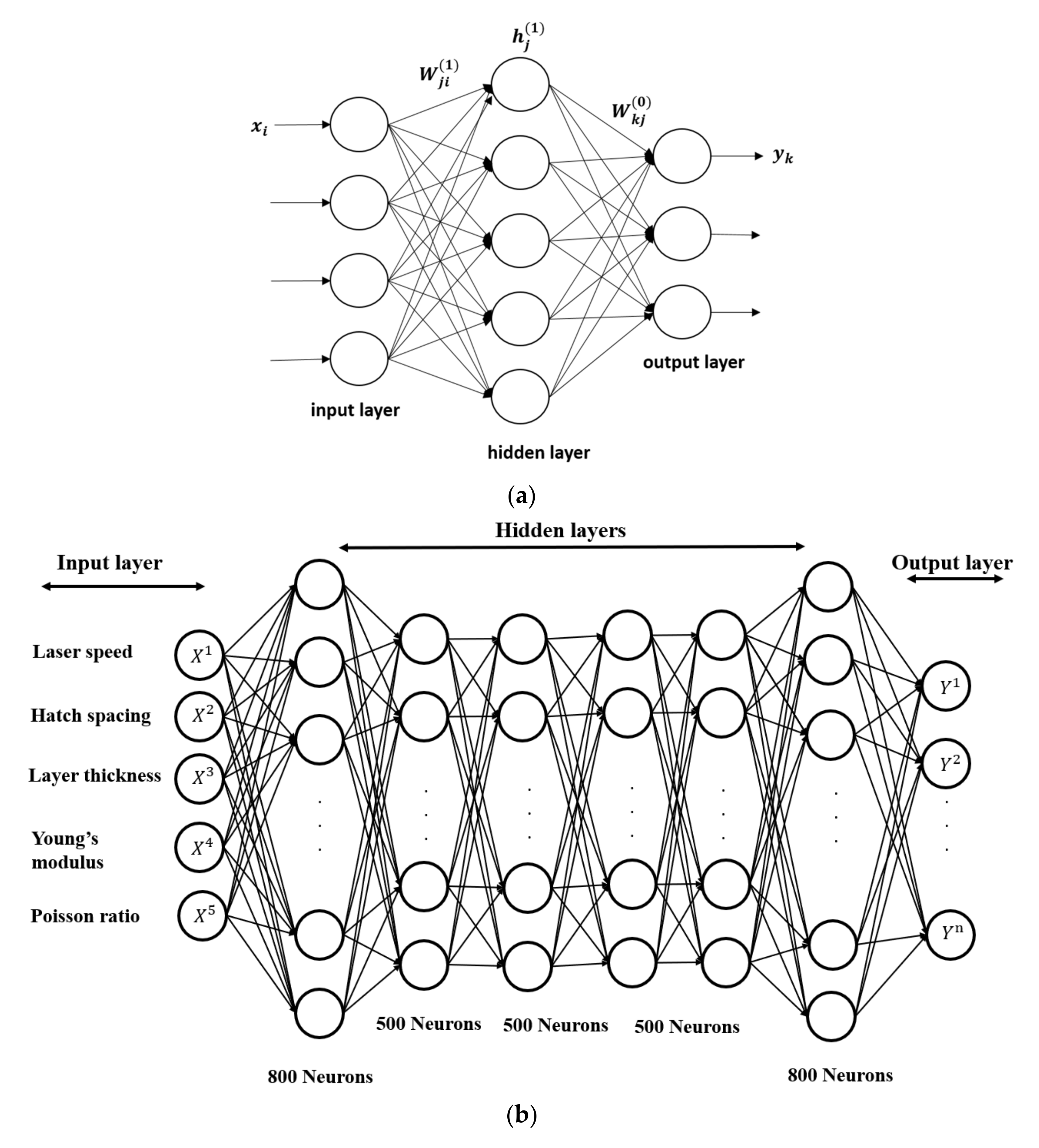
Deep neural networks (DNNs) are a class of artificial neural networks (ANNs), similar to a human brain’s neuronal network. The basic unit of an ANN is called a node, which collects information from one end and passes it to another node at the other end. A node contains the values of inputs, sums their weighted values, and then uses an activation function to produce an output [
29]. A simple structure of a neural network is shown in
Figure 2a. The nodes are arranged in a number of layers. Each layer is fully connected with its subsequent layer, but the nodes in a layer are not interconnected. The first and last layers of an ANN structure are called the input and output layers. The number of nodes in the input and output layers is equal to the number of input and output variables, respectively. After the first layer, there are one or more layers called the hidden layers [
30]. A neural network model with more than two hidden layers and many nodes is referred to as a deep neural network [
31].
The values from each layer are mapped to the nodes in the successive hidden layers by being multiplied by some weights. The new value in each node is given by the equation:
where
k represents the number of layers and
are the weight parameters associated with each node
i whose state is given by
. The
is the activation function that helps to introduce the non-linearity and
are the biases parameters. The sigmoid and hyperbolic tangents are the most widely used activation functions. Once the activation function is selected, we need to determine the optimal weights and biases by minimizing the loss function. The mean square error (MSE) is used as a loss function in the present study:
where
represents the total number of input parameters:
. The
represents a dataset for a given input sample vector. The corresponding target outputs are represented by
and
represents the desired output. In the MSE equation, a regularization term is added to prevent the neural network model from overfitting. Thus, a complete MSE equation can be written as:
where
represents the regularization hyperparameter. In the current study, a total of six hidden layers were considered as shown in
Figure 2b, where the first and the last layer had 800 neurons, and the middle four layers had 500 neurons each. To build our neural network model, we used Matlab’s deep learning toolbox [
32].
3.1.2. Polynomial Chaos Expansion
A polynomial chaos expansion (PCE) is a way of constructing an analytical model that maps the outputs of interest to inputs using a predefined basis of polynomials. The function is represented in the form of a polynomial expansion [
34]. In a PCE, we assume a deterministic map, M, such that the response is
= M(
) where x
,
, and
represents the input and output varibles respectively For simplicity let us consider
to be 1. The probability distribution of
is given by the probability density function
[
35]. Thus, the polynomial expansion of
can be written as the following equation:
where
represents the expansion coefficients. The value of
depends on the order of polynomial
and the number of input variables
. Thus, the exact value of
can be calculated by
. The other term in Equation (13),
, represents the multivariant basis functions, which are orthogonal with respect to the probability density function
, that is:
Here,
represents the Kronecker symbol. For independent input variables, the value of
can be obtained by the tensor product of the univariate orthogonal polynomials
, as in:
where,
represents the multi-index vector. The univariate polynomial basis function was selected with respect to the type of probability density function. For example, if we have a uniform distribution, the Legendre polynomial is considered the optimal basis function. The PCE coefficient
can be computed using a regression approach, by minimizing the mean square error
. Given a dataset D of
N input variables
and their corresponding output vector
, the expansion coefficients can be calculated by solving the following problem:
where
is the regularization factor,
I is the identity matrix and
is the design matrix, whose components are
The total number of sample input points are calculated using
while
represents the oversampling parameters that control the accuracy of the PCE. To generate the dataset, we can use any sampling method, including Latin hypercube or Sobol [
36]. Once we obtain the expansion coefficients, we can use the relationship (13) to approximate the outputs for any input variables.
3.2. Optimization
To find the optimum parameters for an SLM process, we considered three different optimization algorithms: genetic algorithm, particle swarm optimization (PSO), and differential evolution. These algorithms are briefly described in the following subsections.
3.2.1. Genetic Algorithm (GA)
The genetic algorithm is one of the most widely used optimization techniques. Unlike the other gradient-based methods, a GA does not require an objective function to be continuous and differentiable [
37]. The gradient-based methods are not capable of handling discrete variables, and they find it difficult to locate the global minima for a multimodel objective function. The GA is an alternative way to find the optimum solution with some supremacy, especially when dealing with the complex problem of fitting many loops simultaneously.
A GA is based on random walk methods, which require a random search to find the optimal solution. However, this method is not entirely random, as it uses information from the last iteration. The technique is categorized as a guided random search method. The GA methods start with a set of initial points instead of one point in the search area, and so they have a higher chance to find the universal minima for the problem. Genetic algorithms are similar to the biological evolution theory [
38], based on the principle of survival of the fittest, where the universal population undergoes many transformations, at some point in time when the population is not changing anymore, and the best individual among the population is considered as the best solution.
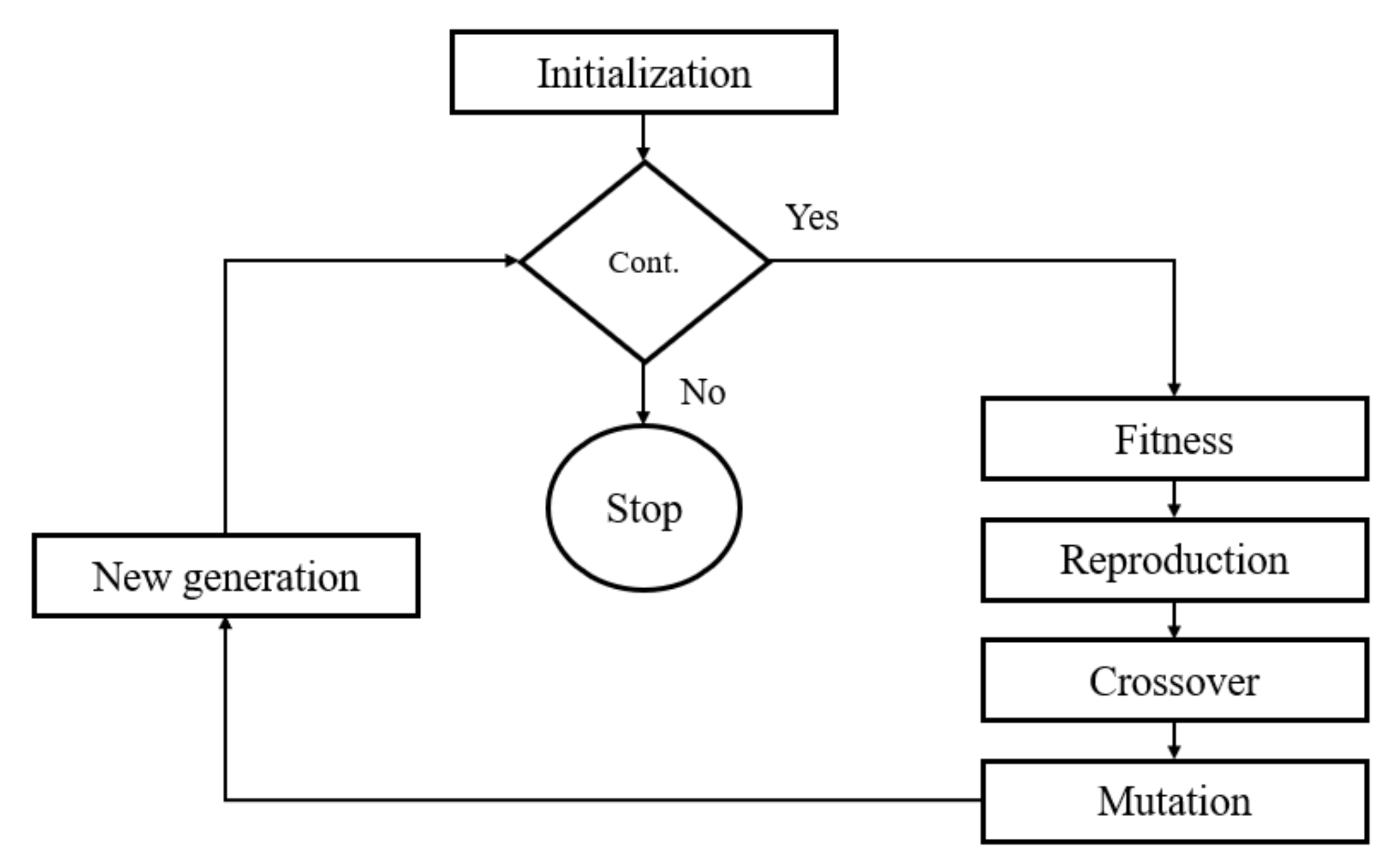
A GA imitates the genetic process in which the characteristics of the parents are transferred to the child. As shown in the flow chart of a GA presented in
Figure 3, it can be divided into four parts: initialization, fitness, selection, and combination. At the beginning of the GA, a set of the initial population or a sample set is generated, and then for each input variable, their fitness value (the value of the objective function) is calculated. The lowest values are taken as the parents’ for the subsequent iterations, and they will produce new offspring for the next iteration [
38,
39]. For example, human genes have chromosomes, so when they make a new child, some chromosomes from the female mix with the male chromosomes and give a new set of chromosomes to their offspring, which has some properties of each parent. Similarly, in a GA, individuals with the least function value will undergo crossovers and mutations to produce better offspring than the parents. By better, we mean their function value is less than their parents’ function value(s). In our present case, a single-point cross-over of 0.8 was established, and the mutation probability was taken as 0.1 to obtain the best results.
In addition to the GA, we considered two other optimization algorithms, particle swarm optimization (PSO) and differential evolution (DE). Both algorithms are similar to the GA, where we start with a population set and try to find the least objective function value for each individual. Each algorithm is explained in the following subsections.
3.2.2. Particle Swarm Optimization (PSO)
The PSO technique uses a large number of samples to explore the optimal solution, as with GA techniques. A GA is based on a biological evolution process, whereas PSO is based on natural phenomena such as birds flocking or fish moving in a group together. PSO keeps a record of the best position of the individual and of the population using the objective function. In a PSO, ‘
pbest’ and ‘
gbest’ denote the best objective function for the population and for the group, respectively [
37]. The velocity for each individual in a population is calculated using ‘
pbest’, ‘
gbest’, and its initial velocity. The new position for each individual is then calculated with the help of the initial positions and their velocity. Each step for the PSO algorithm is described below.
If we assume the ‘nth’ individual in a set, then its position is given by:
and
are the bounds for a variable
, and
represents a random number between 0 and 1. The fitness value of the nth individual can be calculated by:
In the beginning, the best fitness value (
) for each individual is
, and the global best value can be calculated as:
The new velocity for the individual can then be calculated as:
where
, and
are the tuning factors, which are 0.8, 2, and 2, respectively, in our study. Now, the new position can be calculated as:
Based on the new position, we can evaluate the new fitness value, which is:
If the new fitness value is less than that of
, then it is replaced with the
. The global fitness value is computed as:
3.2.3. Differential Evolution (DE)
Differential evolution (DE) is another optimization algorithm that, similar to GAs, is based on an evolutionary process. DE has gained in popularity in recent years for its success in optimization problems in different fields of science and engineering. The algorithm was first introduced by Storn et al. [
40] in 1995 to optimize the non-differentiable and non-linear continuous function. DE algorithms are based on stochastic population-driven evolution methods similar to the other evolution methods. This approach uses a population set and searches the whole design space to find the optimal solution using crossover, mutation, and selection operators. One of the differences between DE and the other evolution methods is the mutation strategy used by DE, which applies to each point and explores the whole design space based on other individuals’ solutions. Georgioudakis et al. [
41] presented several DE algorithms based on different crossover and mutation strategies. There are three controlling factors in a DE algorithm: the crossover rate, the population size, and scaling factors, which all must be controlled to get the best performance [
42].
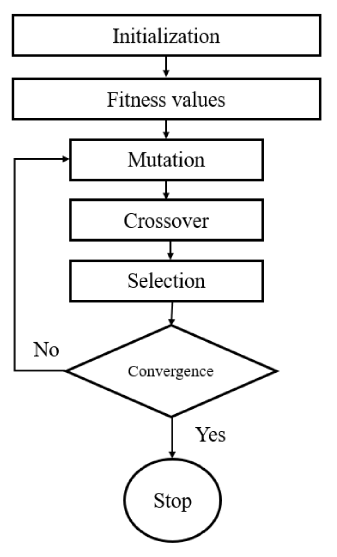
Figure 4 outlines the functioning of a DE algorithm. From mutation to the selection, all steps are repeated until the termination criteria are reached. Our study considers the crossover and the scaling factor to be 0.8 and 0.6, respectively.
4. Application to an Additive Manufacturing Benchmark Test
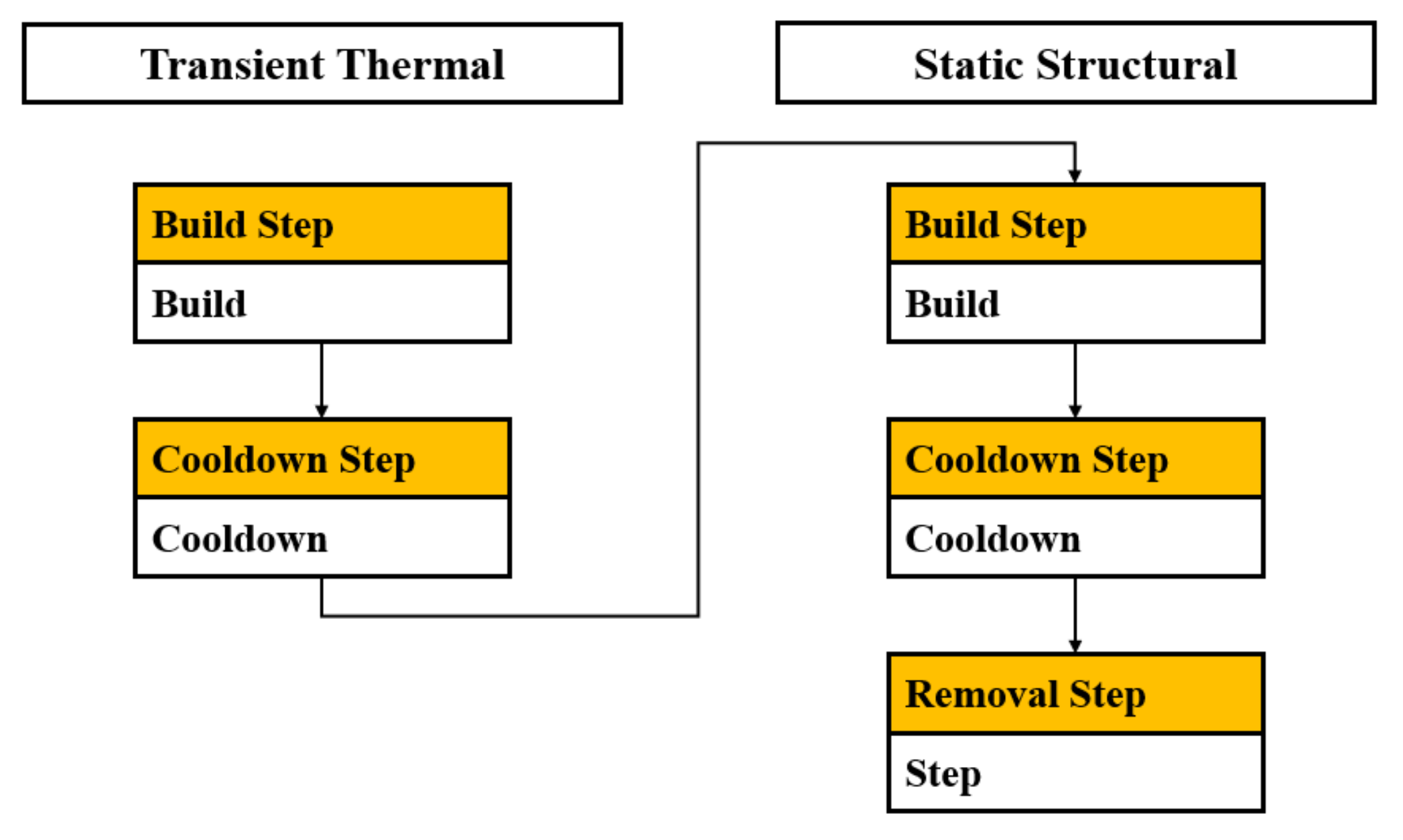
To model the SLM process, we used Ansys additive software [
43] that employs a thermo-mechanical coupling method to simulate the SLM process, as shown in
Figure 5. The heat transfer analysis provides the transient temperature field that is transferred to the mechanical analysis model [
43]. The same workbench additive model has been used in many similar studies [
44,
45,
46] to validate the code and to optimize the SLM build part.
To set up an AM simulation in Ansys, we can either create our geometry in the software or we can import the stl. format of the geometry. In addition, the software gives the freedom to create supports during the simulation, or it can generate them automatically depending upon the given conditions. However, in this study we did not consider any support structure. After the geometry setup, the whole domain was divided into several layers depending on the layer thickness. To simulate each layer, we used the cartesian coordinate mesh with an element birth method to activate the elements in each building step. The numerical model sets the elements in the whole layer to the melting temperature at once, assuming that the developed temperature is always at or above the melting temperature but it does not significantly exceed it. During the melting of the powder, the scan pattern is not considered as an input parameter. Additionally, the unmelted surrounding powder is not explicitly modeled, instead the heat loss between the powder and the solid material boundary is simplified using the convection boundary condition at the interface. A convection boundary condition was used for each heating and cooling step, but the radiation boundary condition is not considered in the model. The powder and the gas convection coefficients were 1.8 × 10
−5 W/mm²·°C and 2.4 × 10
−8 W/mm²·°C respectively. The pre-heat powder temperature was set at 80 °C whereas, the chamber and the base plate temperature were maintained at 40 °C and 80 °C respectively. The other process parameters related to the machine and the material are described in the following subsections. Further details can be found in [
47,
48].
To validate the numerical results presented in this work, we compared the strains and the part deflection results with the experimental data of a benchmark case, AMB2018-1, provided by the National Institute of Standards and Technology (NIST) [
48]. In 2018, the NIST provided a set of experimental results for different additive manufacturing processes, including SLM. All the details about the experimental setup and the operations for AMB2018-1 are available on the NIST website [
9]. This benchmark study aimed to provide reliable stress, strain, and deflection benchmark data in a bridge-like structure.
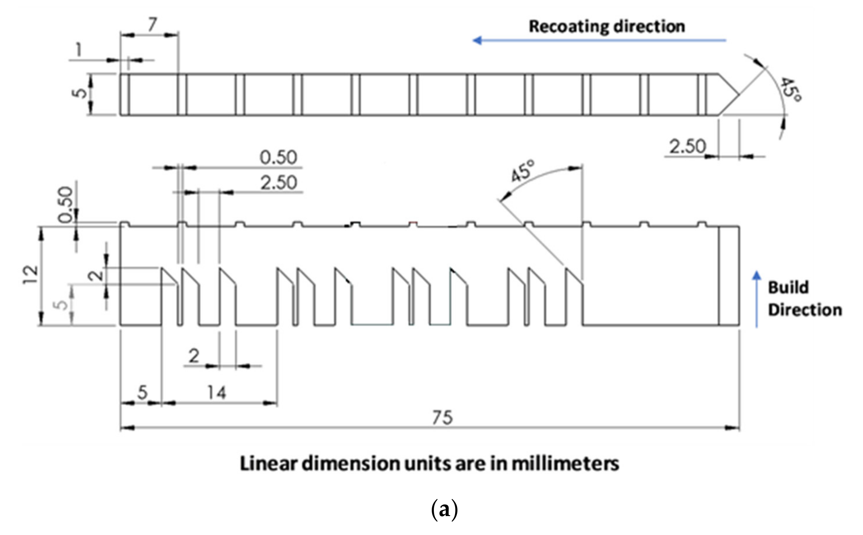
A brief description of this benchmark case, shown in
Figure 6a,b, is provided here. The residual stress and strain data were measured using x-ray diffraction and neutron diffraction methods. For the part deflection measurement, the bridge was partially separated from the base plate, and then a coordinate measurement machine was used to measure the deflection. The AM part was constructed using two different machines: the NIST in-house-built machine AMMT (additive manufacturing metrology testbed) and the EOS M270. In the present study, we considered only the EOS M270 machine, as the measurement results for the part deflection were not available for the structure constructed with the AMMT. More details on the process can be found in [
48]. The test case comprised four bridge structures on a build plate, as shown in
Figure 6b. All four bridges and the substrate were constructed using IN625 material with a powder bed fusion process. During the process, the bridges were built with some spacing (
Figure 6b). As the bridges’ construction process does not affect the other bridges’ properties, we considered only one bridge on the substrate for our numerical simulations as shown in
Figure 6c. This simplification significantly reduced the computation time. The bridge and the build plate’s final dimensions were 75 × 5 × 12.5 (mm × mm × mm) and 81 × 12.7 × 11 (mm × mm × mm), respectively. Our primary objective was to investigate the strain within the build-part in the validation study. In addition, we verified the geometry deflection in the z-direction after part of the bridge was separated from the substrate.
4.1. Baseline Machine Parameters
The AM part and the substrate were constructed using a Nickel alloy, IN625. In the experiment, the part was built at the center of the substrate, with odd and even layers that were melted using horizontal and vertical scan strategies. However, because of the software constraint, we only considered the horizontal strategy for all the layers.
Table 1 shows the machine parameters that were used during the SLM experiment.
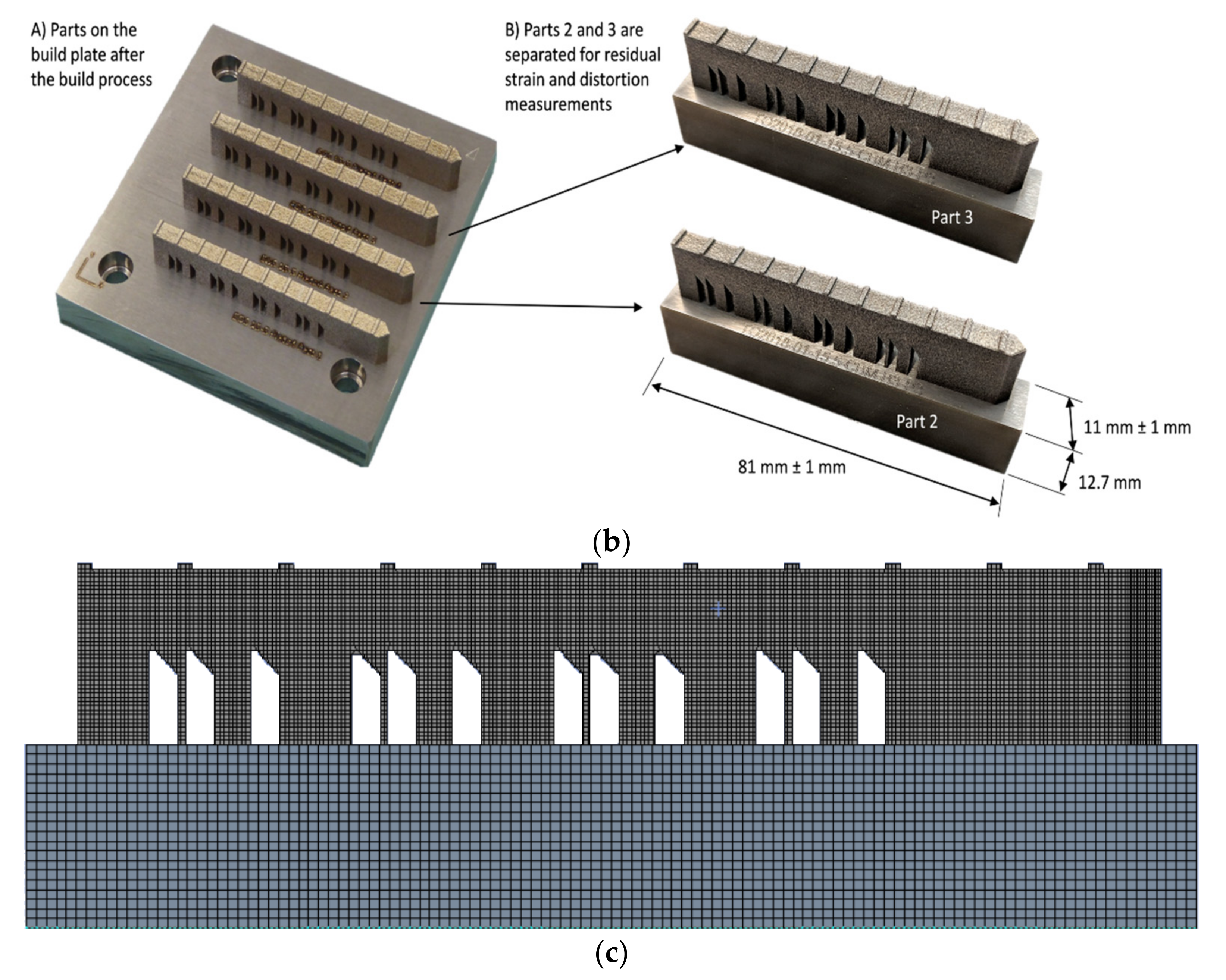
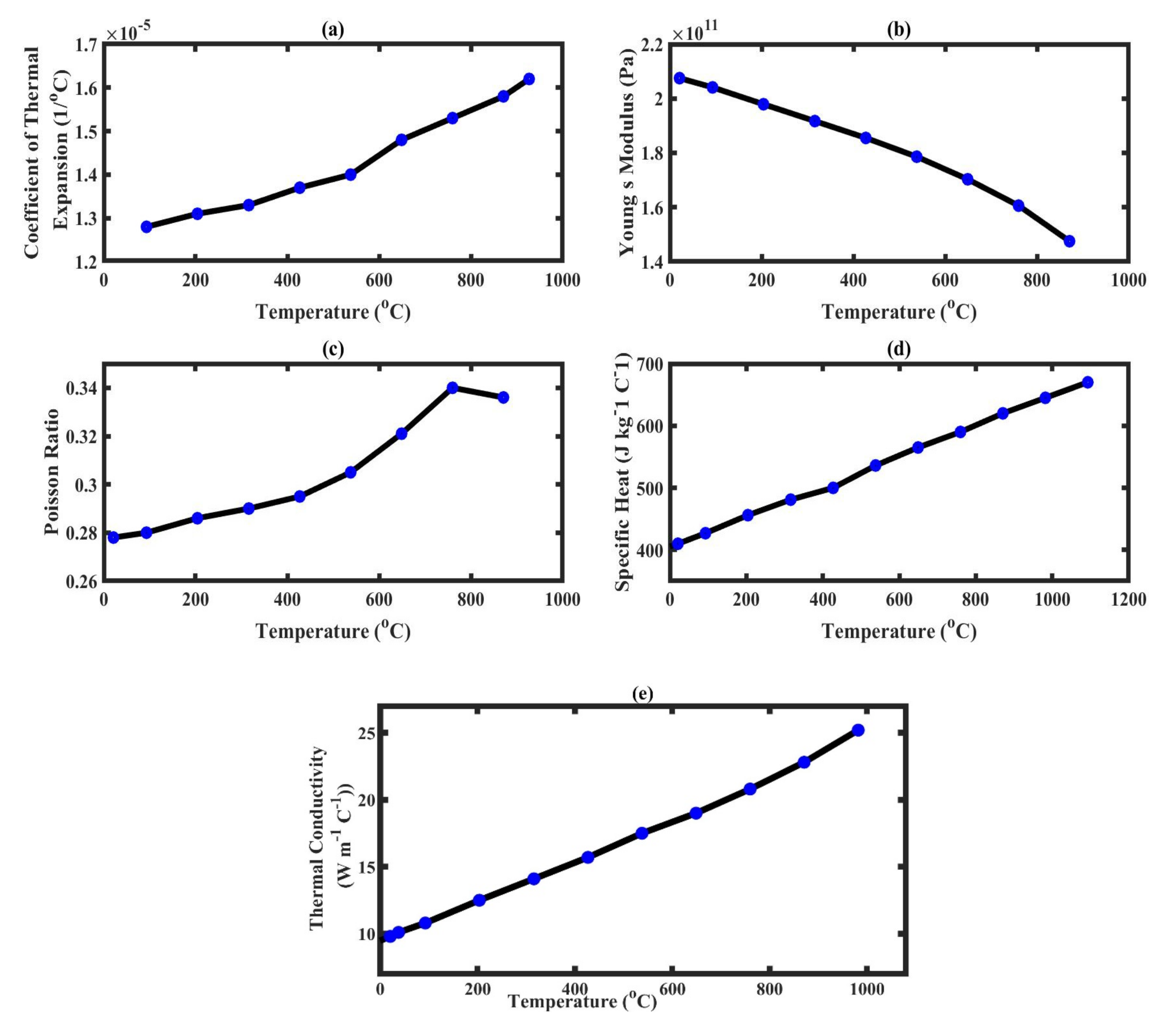
4.2. Baseline Material Parameters
IN625 is a very common alloy used in manufacturing. Therefore, its properties are easily available and well-known. In this work, we considered the temperature-dependent material properties taken from [
49] and presented in
Figure 7.
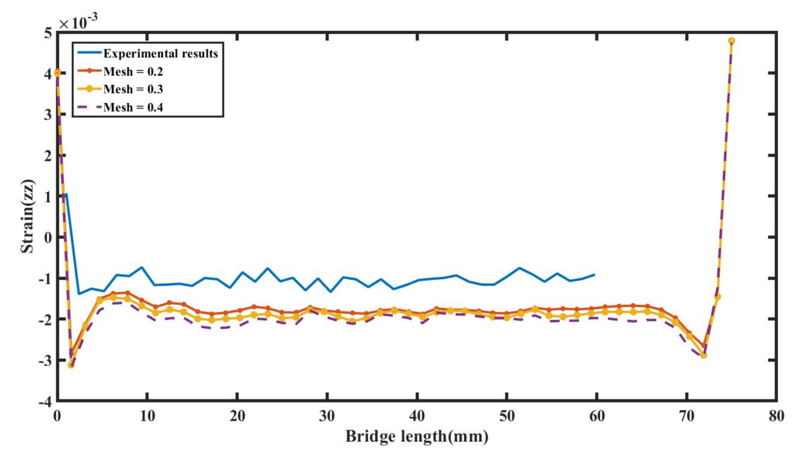
4.3. Mesh Convergence Study
A mesh convergence study was first conducted to evaluate the effect of the mesh size of the 3D finite element model on the simulation results. We selected three different mesh sizes, compared their results with the experimental results, and concluded that a mesh of size 0.3 mm was best suited for further studies. The comparison study was conducted using the residual strain results at z = 9.536 mm. In
Figure 8, the numerical results are similar to the experimental results.
Table 2 presents the decrease in error norm between the experimental and numerical results with mesh size. For the error analysis, we used the
relative error norm which is defined as
in which
and
are the experimental and simulation data, respectively, whereas the total number of data is represented by
. Each simulation was performed on 32 CPUs that each had an Intel E5-2683 v4 processor. From
Table 2, it is clear that the error decreases with the decrease in mesh size, but at the same time, the computation cost increases. Therefore, we chose a 0.3 mm mesh for our simulations, as it provides better results than the 0.4 mm mesh size, while it is much less computationally expensive than the 0.2 mm mesh size.
4.4. Validation of the Finite Element Model
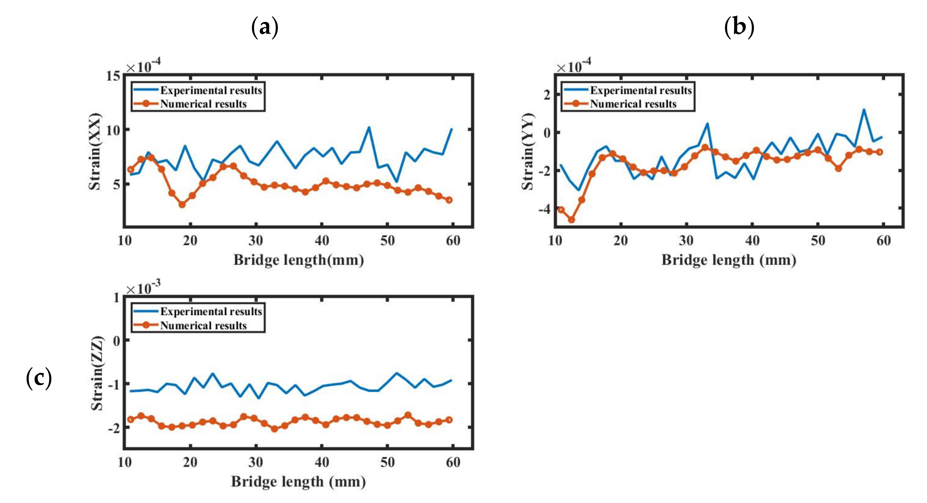
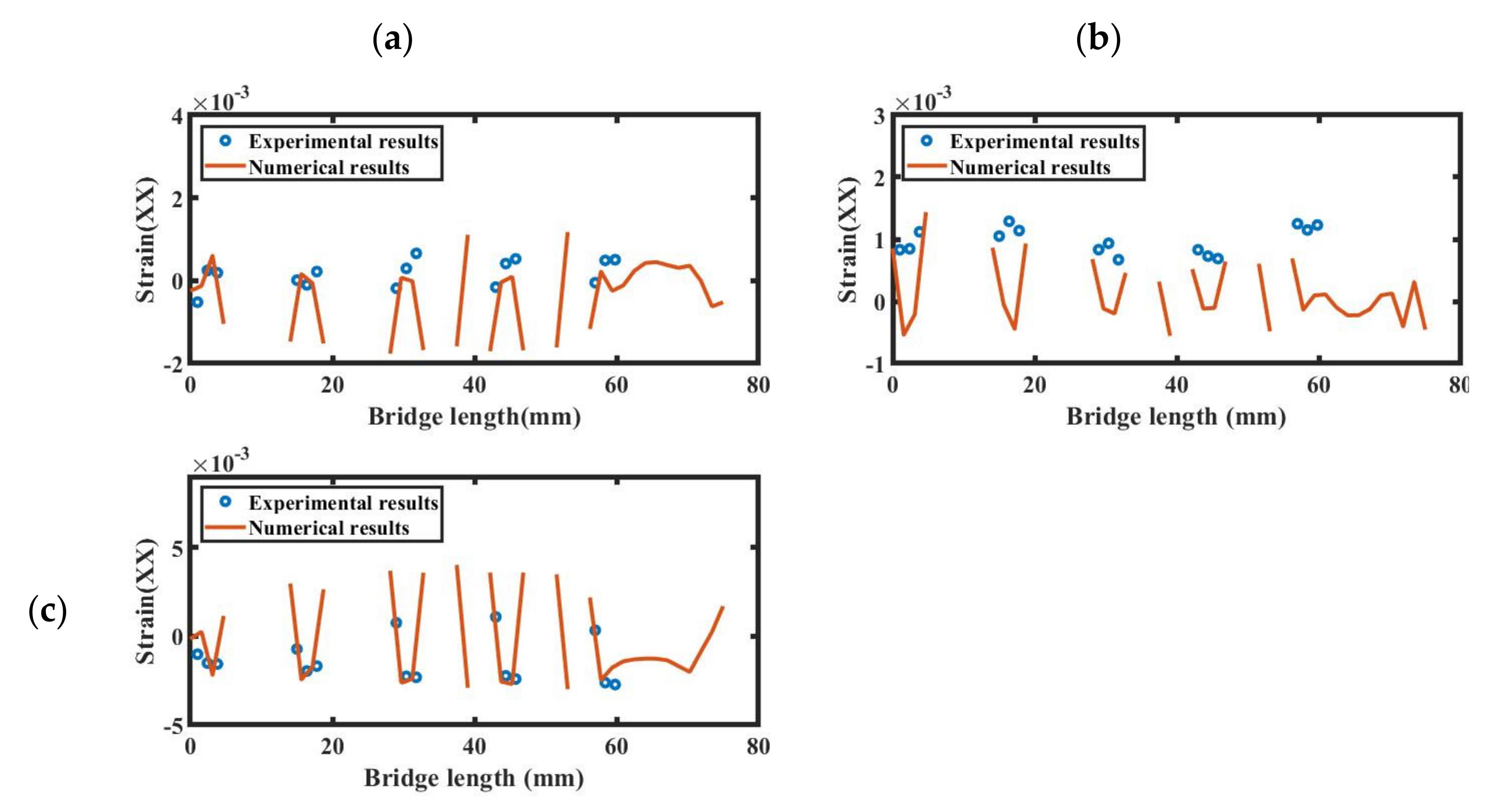
Using the baseline parameters, the simulation results were validated using two different analyses. In the first case study, the normal residual elastic strains were compared with the experimental results at two specific locations (z = 9.536 and 2.216) in the bridge.
Figure 9a–c show a comparison of normal strains in the x, y, and z-directions, respectively, at the line z = 9.536, whereas
Figure 10a–c show that comparison at z = 2.216. The simulation results at both values show a good correlation with the experimental results. It is essential to mention here that the experimental strain results at z = 9.536 were extracted only up to the 60 mm length of the bridge. The relative L2 norm error values for the x, y, and z-direction strains at z = 9.536 were 0.4041, 0.6202, and 0.7820, respectively. The small difference in the results may be due to the different scan strategies used in the experimental and numerical simulations.
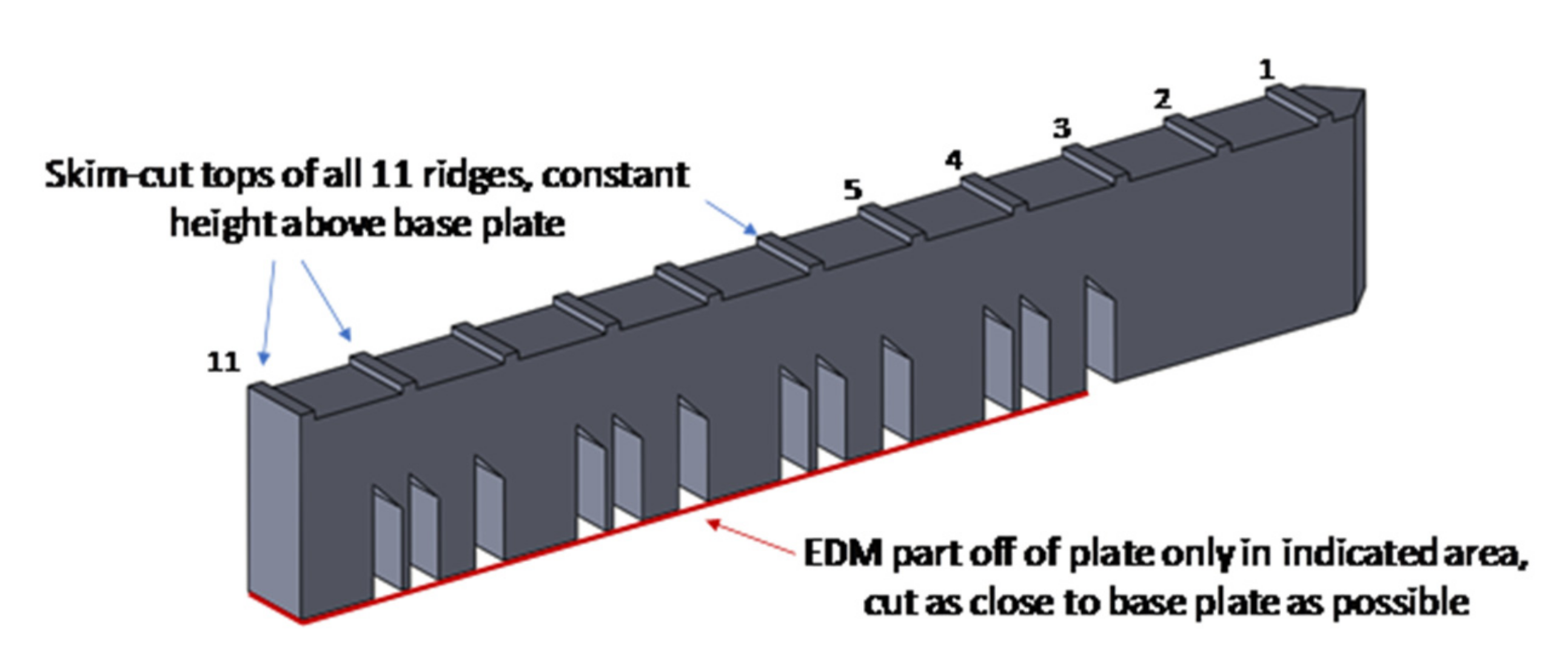
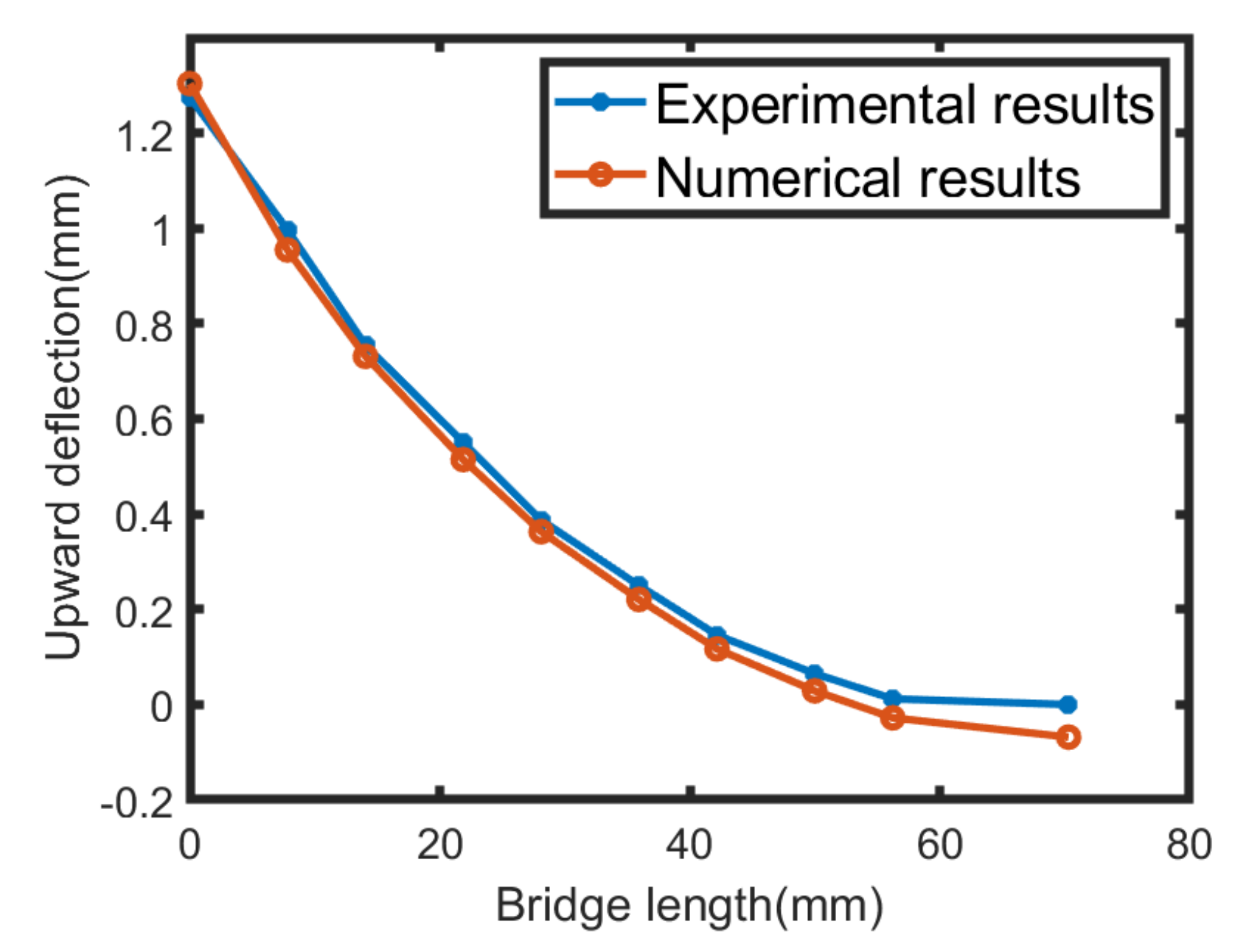
For the second validation case study, we analyzed the deflection of a partially separated bridge from the baseplate as shown in
Figure 11, in which all 12 bridge legs were separated from the substrate. The partially separated bridge was then allowed to move upwards without any external force, except for the internal residual stresses. The deflection of the bridge in the z-direction was measured at 11 ridges on the bridge’s top surface. In
Figure 12, we show the comparison of the deflection results from a simulation and an experimental study. The relative L2 error norm between the simulation and experimental results is 0.0629, proving a good correlation between the results.
4.5. Deep Neural Network (DNN) Surrogate Modeling
A surrogate model was constructed using DNN regression to build a surface map between the input and the output data set. The DNN has six hidden layers, where the first and the last layers have 800 neurons and the middle four layers have 500 neurons each. To construct our DNN model, we used Matlab’s deep learning toolbox.
In the present study, we considered five uncertain parameters, where three are the machine parameters and two relate to material properties. To change the values of Young’s modulus and the Poisson ratio, we multiplied their baseline values by factors
and
, respectively. The input variables were laser speed, layer thickness, hatch spacing,
, and
. A dataset was generated with a sample of 360 input variables using a Sobol sampling technique. Initially, the sample set responses were obtained using the finite element model, and the normal strains were calculated at z = 9.536 (build direction). Later, the outputs from the 360-sample set were used to construct a DNN model, where 70 percent of the data was used to train the DNN, 15 percent was used to test it, and another 15 percent was used to validate the DNN model.
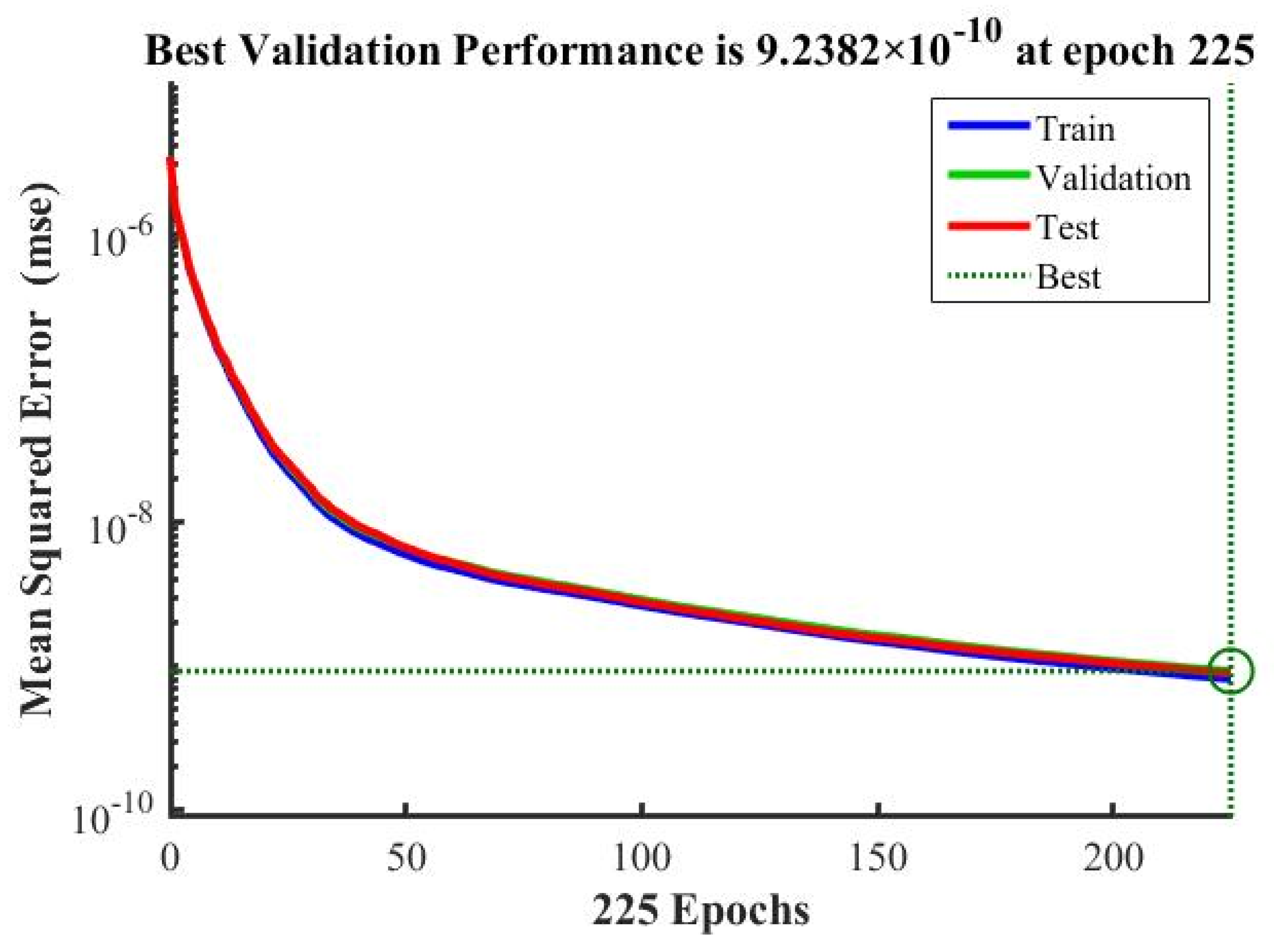
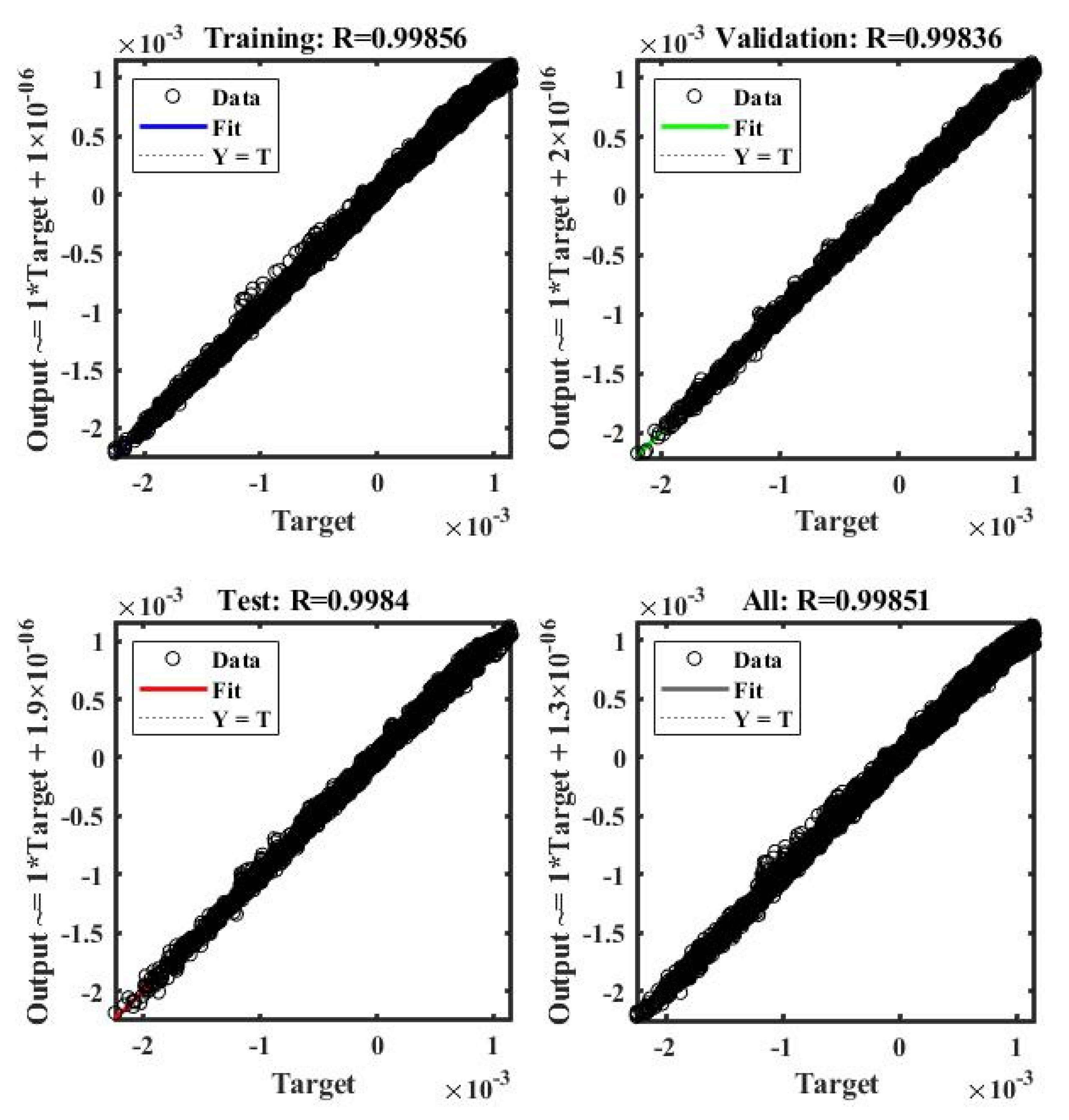
Figure 13 shows the loss drop during training, testing, and validation of the DNN model, and
Figure 14 shows the plot between the exact and predicted values during training, testing, and validation of the model, using x-strains. The DNN model was developed separately to train and predict the outputs of each normal directional strain at z = 9.536.
Figure 15 compares the DNN outputs and the simulation outputs for each directional strain at z = 9.536.
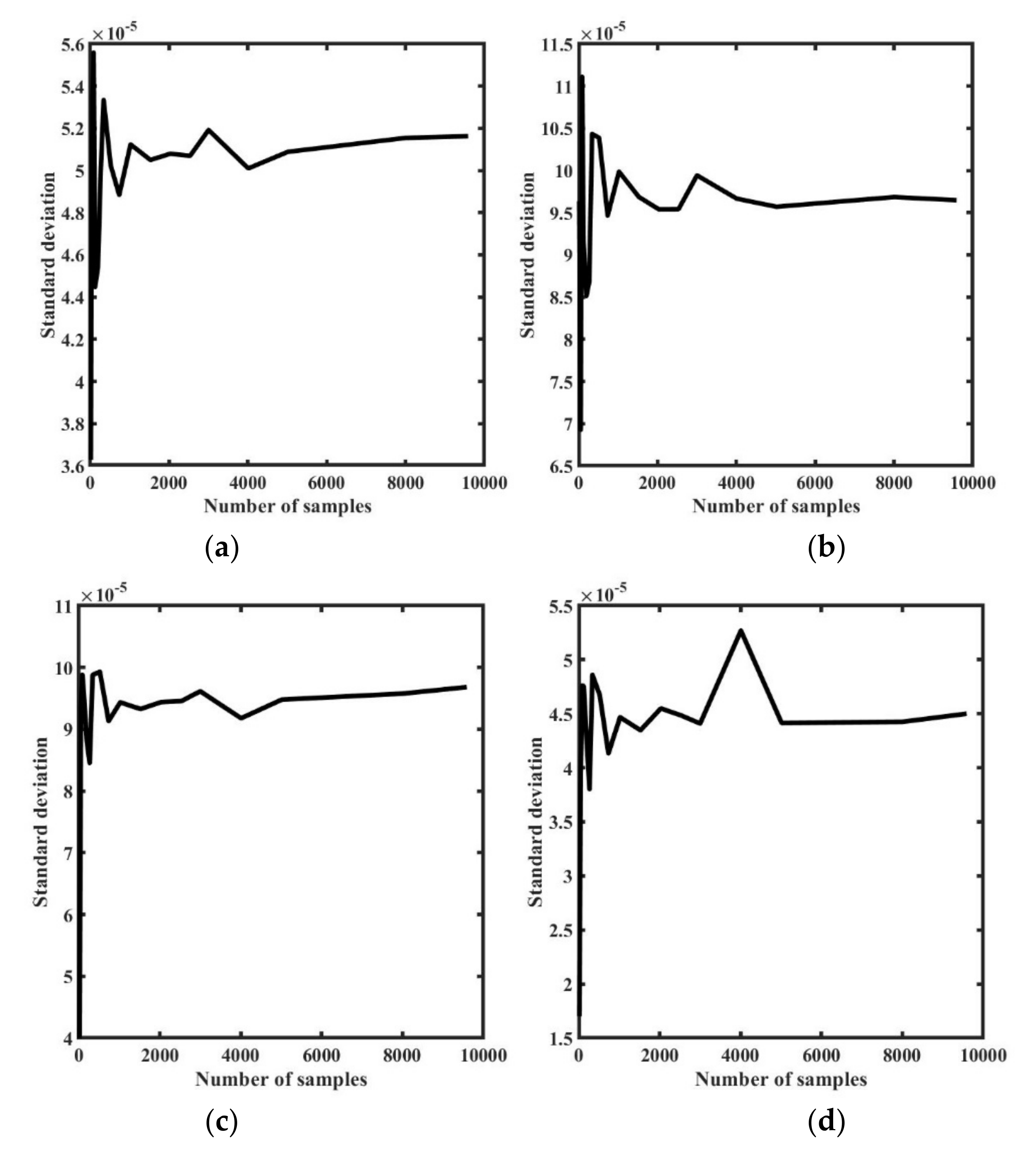
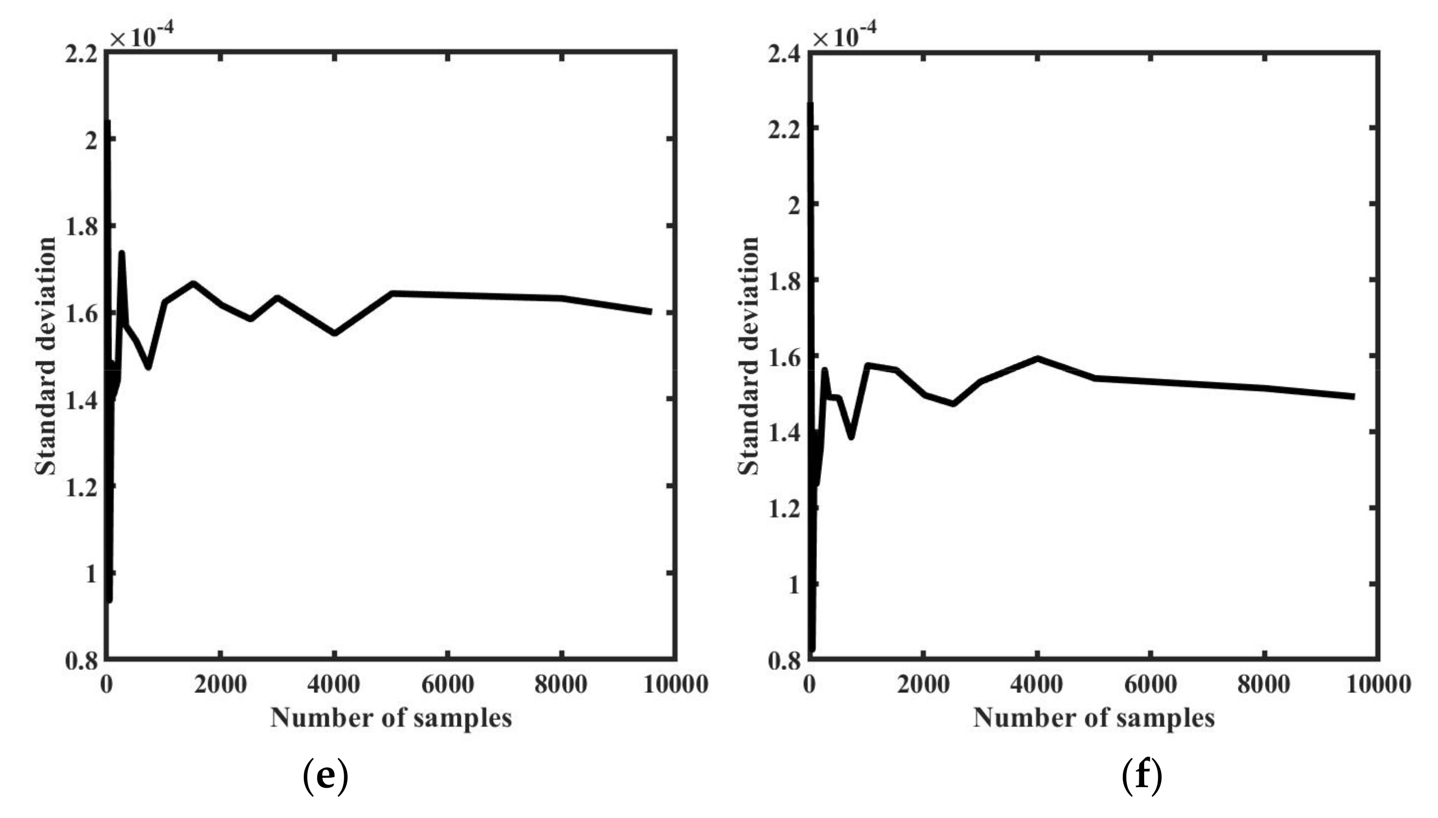
Once the neural network surrogate model is developed, it can be used to perform statistical and calibration studies. For this purpose, a sample of sufficient size must be generated. We used the Monte Carlo method to perform the convergence analysis using standard deviation (Std) for different numbers of sample sets, including 12, 48, 84, 120, 192, 264, 336, 516, 732, 1020, 1524, 2028, 2532, 3000, 4008, 5016, 8004, and 9588, and the standard deviation was calculated for each sample set. The convergence study was performed for individual directional strains at two locations.
Figure 16a,b shows the results for the x strain at 15 and 45 mm, while
Figure 16c–f present convergence plots for the y and z directional strain at the 15 and 45 mm locations, respectively. From the figures, we concluded that a set of 6000 samples was enough to perform the sensitivity and uncertainty analysis for an SLM process, as described in the following sections.
4.6. Polynomial Chaos Expansion
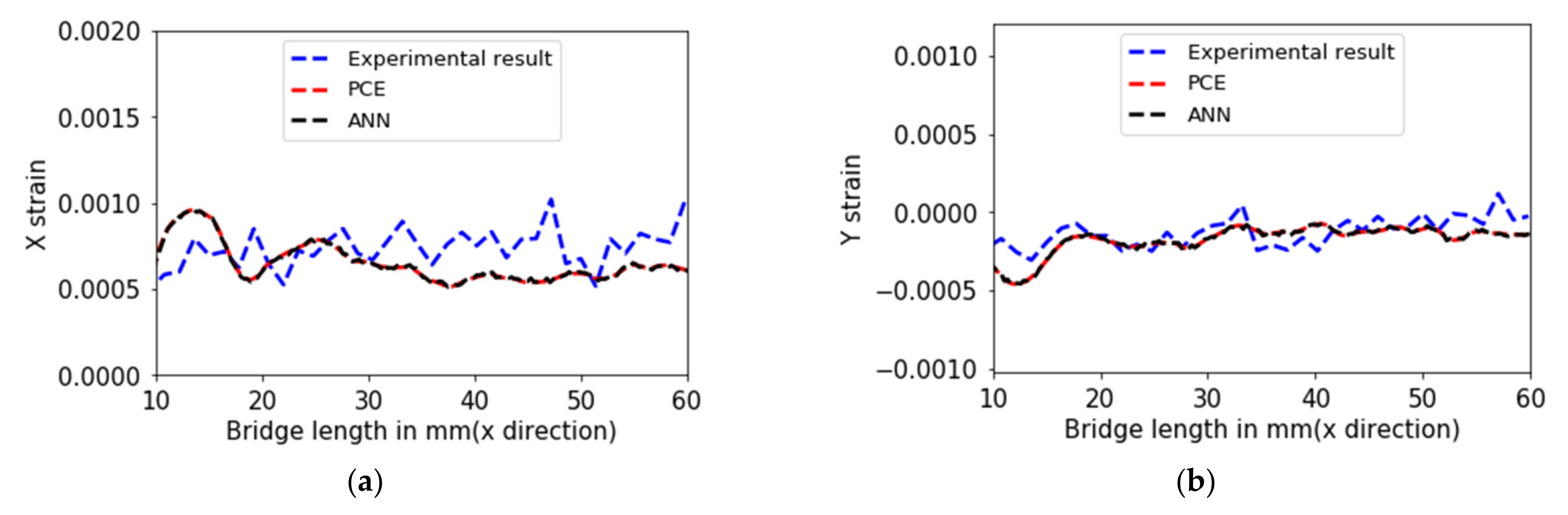
Along with the DNN, we used a PCE model to construct a surrogate model for our SLM process. We conducted this comparative study to determine the best surrogate model for our problem, one that can simultaneously reduce the computation time and increase the accuracy of the predictions. Thus, similar to the DNN, the PCE was trained and tested with outputs of 360 samples calculated using the Ansys additive software. For the comparison, we generated a data set of 6000 input samples with the Sobol sampling technique, and then used our trained PCE and DNN surrogate models to predict normal strains as outputs for the points at z = 9.536.
Figure 17 shows a comparison between the DNN and PCE models, and we can conclude that the results are very close to each other. The mean square error between the PCE and the DNN is 7.17
, proving that both models are equally adequate for prediction. In
Table 3, we present a comparison of the computational cost for both models, and
Table 4 presents the error between experimental and predicted values. The results show that the PCE is faster than the DNN in training g, but almost three times slower than the DNN in prediction. Considering the overall time, the DNN is faster than the PCE. Therefore, in conclusion, we proceeded with our investigation using a DNN instead of a PCE.
4.7. Uncertainty Quantification
For the uncertainty quantification, we used the normal strains in the x, y, and z directions at z = 9.536. The analysis was conducted using Python libraries, which include Numpy, statistics, and other libraries.
To begin, a set of 6000 input samples was generated using a Sobol sampling technique. Next, the trained DNN model was used to calculate the x-directional strains along the line z = 9.536 for these input variables. The samples were generated under ±15% bound on the baseline input values, which are shown in
Table 5. As mentioned before, the values of Young’s modulus and the Poisson ratio were modified by multiplying them with the factors
and
, respectively. The values of these factors lie between 0.85 and 1.15, representing ± 15% variation.
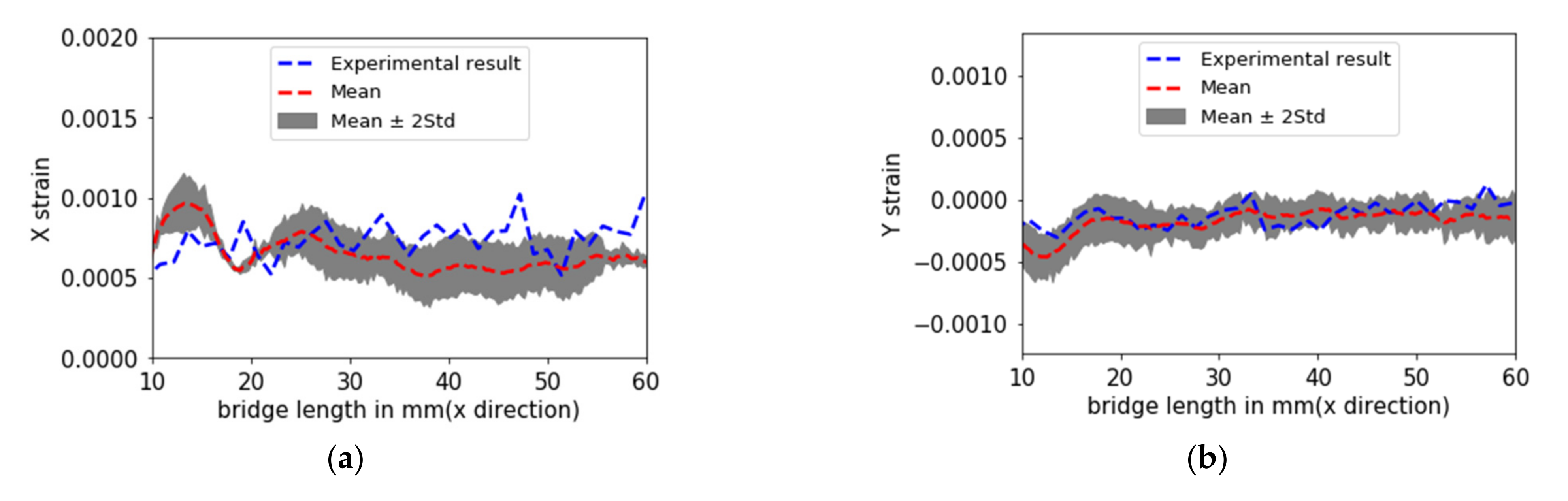
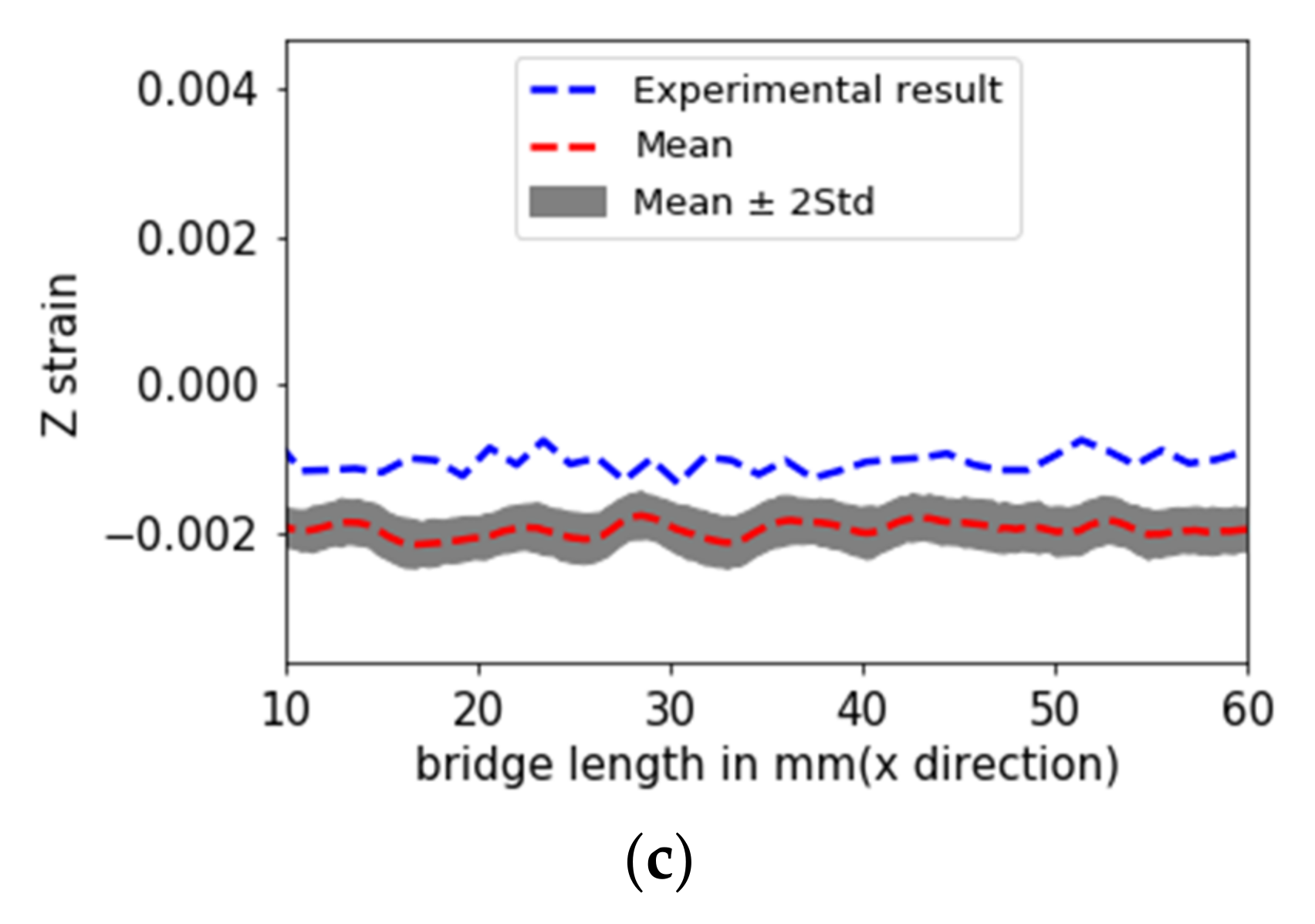
Figure 18a illustrates the uncertainties in the process outputs, which shows that the mean of the data was very close to the actual results; the grey area represents the confidence interval of 95%. The confidence interval was equal to the ±2x standard deviation. A similar study was performed with y- and z-directional strains at the exact location and their analysis plots are shown in
Figure 18b,c, respectively. The L2 error norm between the mean value and the experimental results for Y strains was 0.6662, whereas, for the z strains, the value was 0.8764. The experimental results for Y strains lay in the 95% confidence interval, but for the z strain, they did not. This may be explained by the simplifications and modeling hypotheses used in the numerical software of the model limitations; for example, the model does not consider the anisotropy in the material properties or the laser power.
4.8. Sensitivity Analysis
For sensitivity analysis, we considered five input parameters: three machine parameters and two material parameters. The study considers the primary parameters of layer thickness, laser speed, hatch spacing, Young’s modulus, and Poisson ratio. The input parameters’ effects were measured using the normal strains, and by calculating the first-order Sobol indices for each node. Similar to the uncertainty analysis, the normal strains were calculated at z = 9.536 along the bridge direction in each simulation.
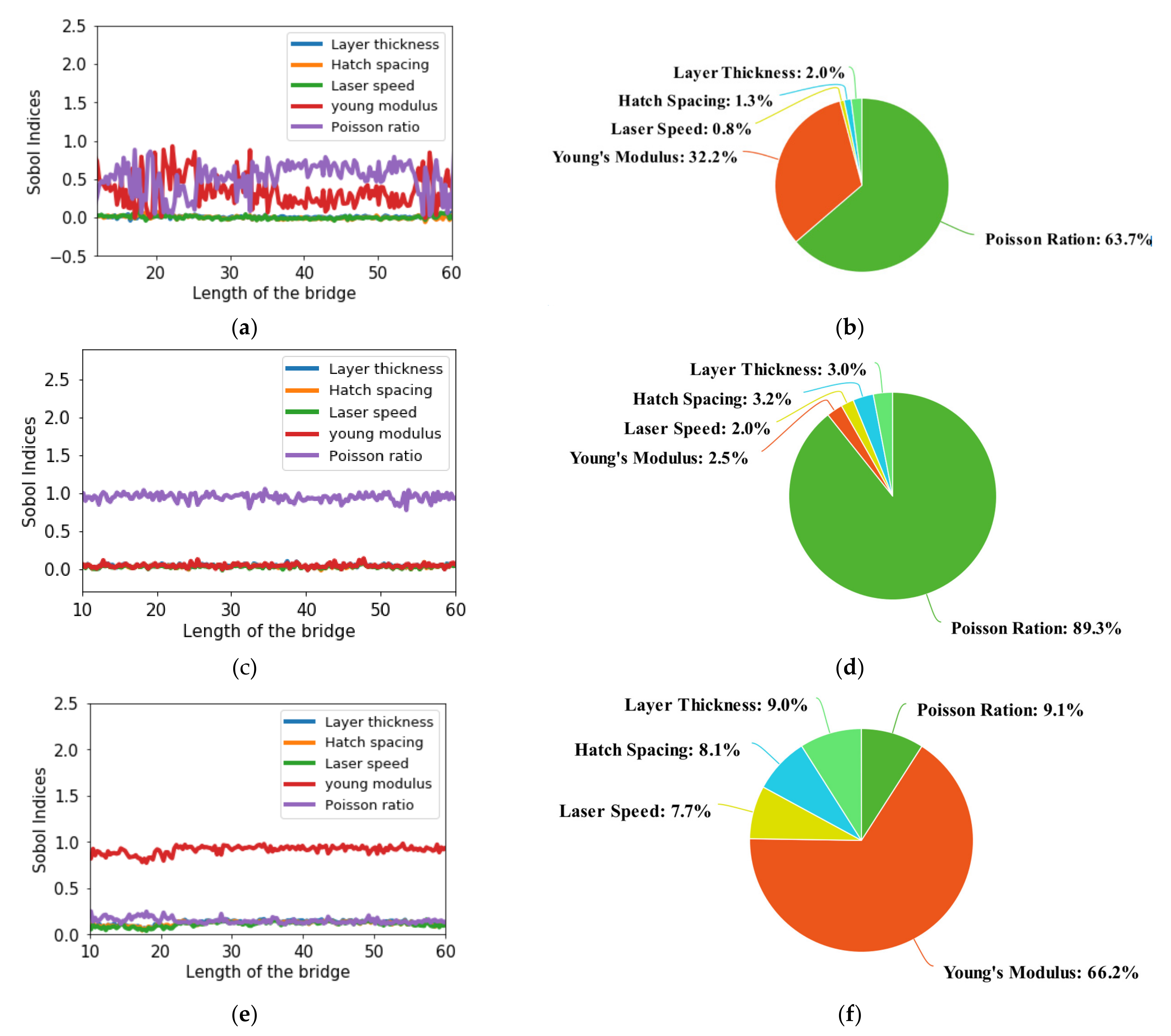
Figure 19 presents the variation in the Sobol indices along the bridge length. A pie chart is provided for each parameter, representing the importance of each parameter as a percentage. From
Figure 19, we can conclude that the Young modulus and the Poisson ratio are the most critical parameters for the SLM and that hatch spacing is the least important parameter among the five parameters considered. If we consider the x-directional strains, then the Poisson ratio and the Young modulus are the most important parameters. While both parameters’ influence changes along the bridge length, both contribute 30% to 65% in the SLM output. The three machine parameters are less influential than the material parameters, but they contribute significantly to the directional strains.
Figure 19b shows the effect of input variables on y-directional strains, indicating that the Poisson ratio is the most dominating factor among the input variables. The Poisson ratio contributes between 86 and 90% in the y-directional strains. The other four parameters are equally essential and make contributions of 2 to 5% to the normal strain in the y-direction. However, the situation is the opposite in the case of z strains, where the most dominating factor is Young’s modulus instead of the Poisson ratio. Young’s modulus is 65 to 68% more important than the other parameters for z strains, while the Poisson ratio is the second most dominant factor.
If we look at all the results we find that the machine parameters are less influential than the material parameters. However, the machine parameters’ effects are still significant in the SLM process. Thus, we cannot ignore their importance in the SLM output, and we need to consider these machine parameters to optimize the SLM output. In the next section, we consider all five parameters and perform an optimization analysis to find the best configuration of the input variables to obtain the optimal SLM to build-part.
4.9. Optimization
We performed an optimization analysis to find the optimized parameters for an SLM process, using GA, PSO, and GE as our optimization algorithms, and the ANN model to generate the required data set for the optimization process, as it is faster than the PCA model. From our sensitivity analysis, we found that all five parameters are essential for the process, and so we considered all five parameters as the input variables. We used 100 as the initial population for the GA algorithm, with 0.8 and 0.1 as the crossover and the mutation probability, respectively. However, in the DE, we took 0.6 for the scaling factor and 0.8 for the crossover.
Table 6 presents the optimized parameters for the SLM process with the different optimization algorithms. From this Table, we can conclude that all the algorithms provide similar fitness values and that the optimized parameters are also very similar. However, the PSO produces results much faster than the other two algorithms. Therefore, using a PSO optimization algorithm with the DNN model to obtain the optimal parameters is highly efficient and less computationally expensive than the other options.
In
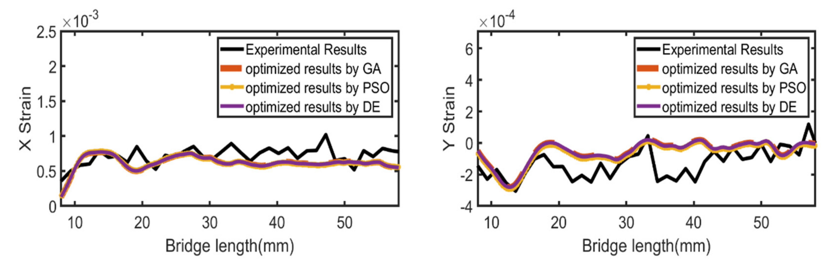
Figure 20 we present the SLM outputs for the optimized parameters obtained from all three optimization algorithms. We used Ansys additive simulation for each set of optimized parameters obtained from all three algorithms and plotted the normal strains along with the experimental results. From
Figure 20, we can conclude that the results are similar and very close to the experimental results.
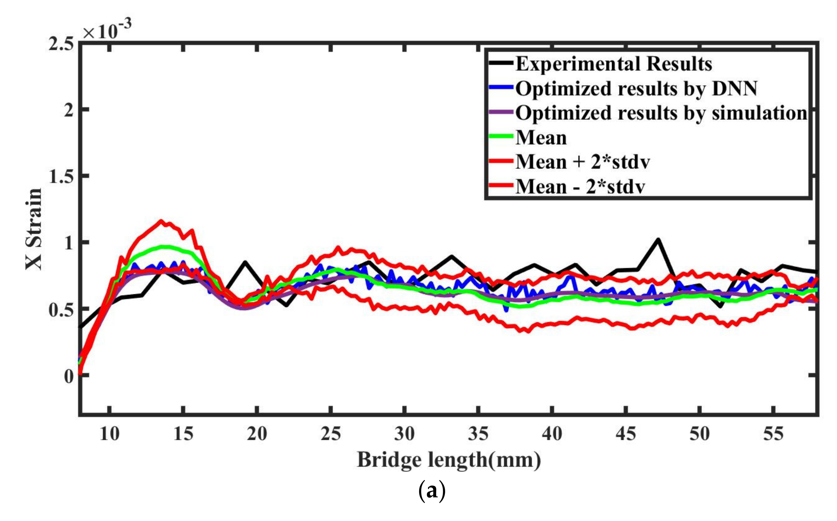
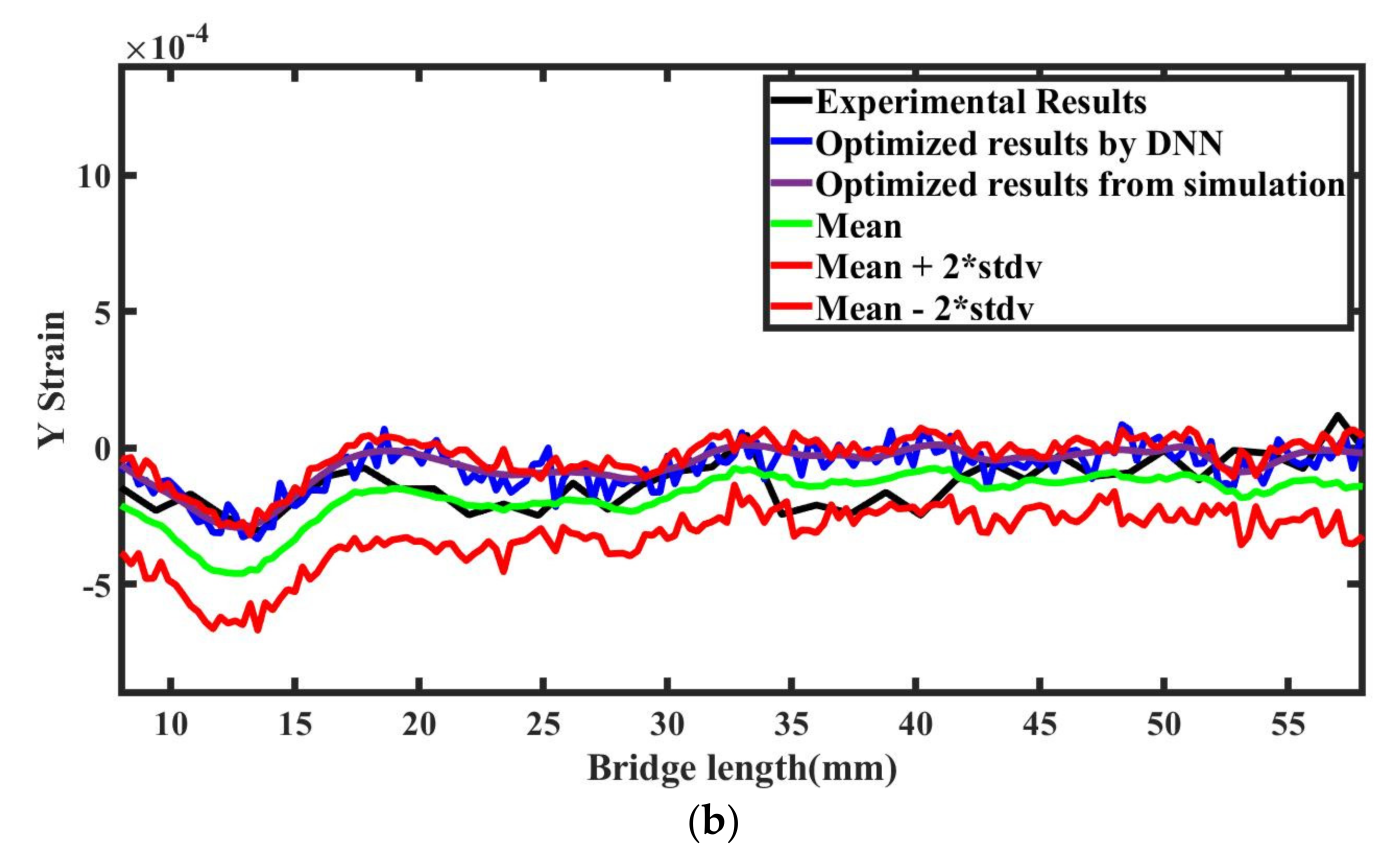
Figure 21 compares the optimized output results obtained from the simulation and from the DNN model. The L2 error norm between simulation and a surrogate model is 0.0965 and 0.2264 for x and y directional strains, respectively. The figure proves the efficiency of the DNN model and the optimized results, which lie in the 95% confidence interval.
5. Conclusions
In this paper, we presented a framework to analyze and optimize the SLM process other than the more widely-used experimental and numerical techniques. We used machine learning (ML) methods with the SLM numerical model to study the sensitivity and uncertainty during the additive process. Neural networks and polynomial chaos expansions were the primary machine learning methods that we considered. The dataset of full-order numerical solutions was performed using ANSYS additive software and the results were validated using publicly available experimental results. The 3D thermo-mechanical finite element model was used to solve a set of 360 samples created using the Sobol sampling technique. The outputs from the 360 samples were then used to train and test the surrogate models. We found that the deep neural network model was faster than the PCE model, so we adopted the DNN model for the rest of the analyses. Once the DNN model was trained, it was combined with the Monte Carlo technique to find the number of simulations needed to perform the sensitivity and uncertainty analyses in the SLM process. The standard deviation convergence plots for each sample set helped us to conclude that 6000 samples are sufficient to perform the study. The sensitivity analysis revealed that the Young’s modulus and Poisson coefficient are the most critical parameters during the process, while the layer thickness, laser speed, and hatch spacing are less important. However, the machine parameters still hold significant importance (5% to 10%). As all the parameters hold significant importance in the SLM process, we considered all five parameters for the optimization analysis. The surrogate DNN model was utilized to optimize with three different algorithms: GA, PSO, and DE. The results were compared, and all three algorithms were found to be equally good at calculating the optimal solution; however, PSO took the least time. The combination of DNN and PSO for optimization provided good results and incurred significantly less computation cost. In the future, as an extension of this study, we will work with the physically informed machine learning models to improve results.


