1. Introduction
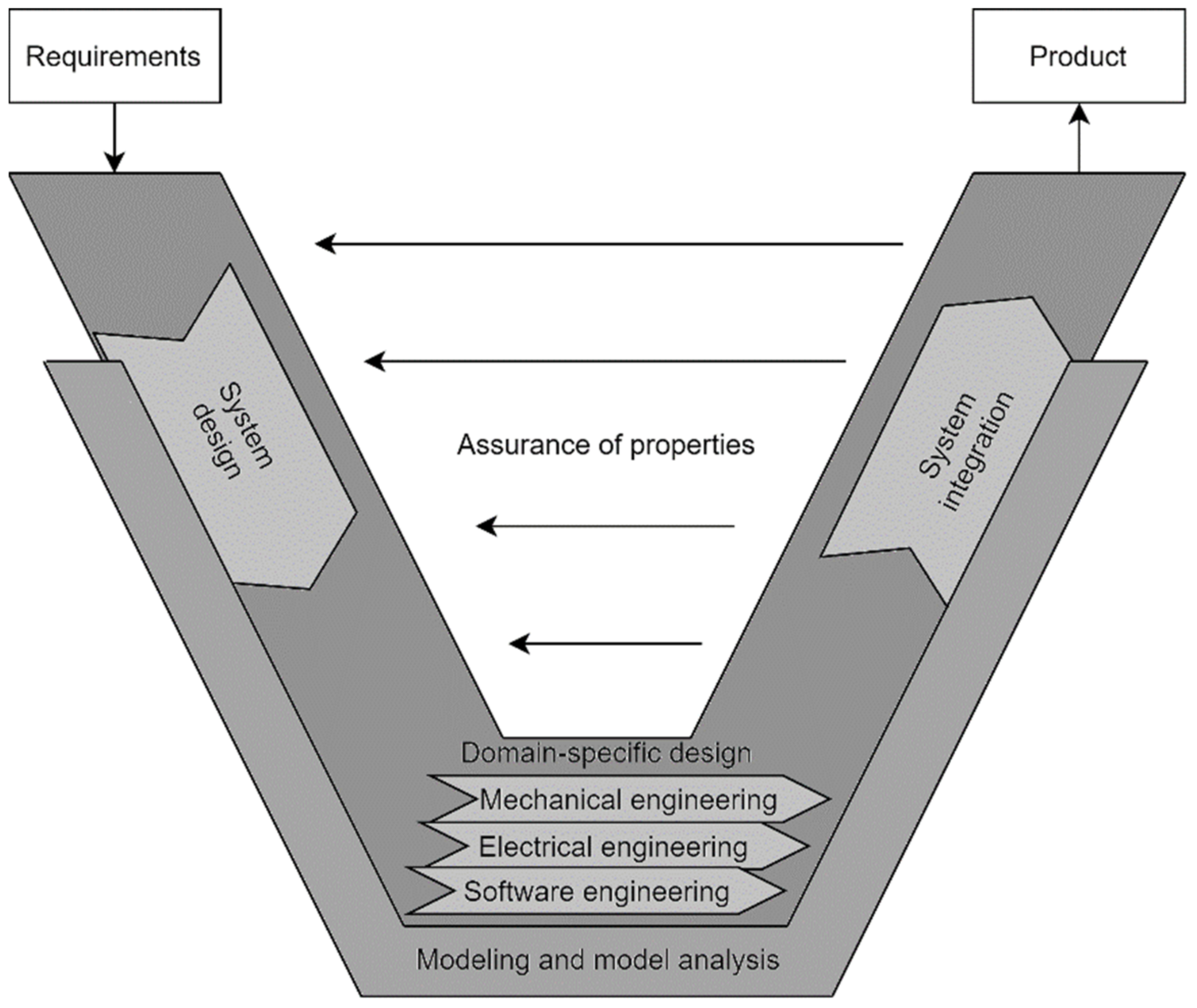
The V-Cycle (
Figure 1) as defined in the VDI 2206 guideline is a systematic approach for the development of a mechatronic system [
1]. The V-Cycle or V-Model is represented by a seamlessly following development stages and gradual verification and validation. The initial stage is a precise definition of the system requirements. The next step involves an analysis of the requirements and development of the general design of the system, with the support of system engineering tools and languages such as SysML or System Composer [
2,
3]. The general solution concept of the system is then split into specific domains of mechanical, electrical, and software engineering to be further concretized and then integrated to form an overall system. At this point, the interaction between the domains needs to be investigated. The design process is continuously verified and validated. The result of this cycle is a verified and validated product. The entire development cycle is also supported with modelling and simulation tools and follows the model-based design methodology [
4,
5,
6].
If the development cycle has been strongly supported with modelling and simulation tools, after the domain-specific design, we have designed a simulation model of the mechatronic system and its control strategy. In case we decide to proceed with this design to the system integration phase, we need to check whether the designed control algorithm could be performed on a desired hardware in real-time [
7,
8]. Since testing the control algorithm on the real prototype can be dangerous in many scenarios, it is efficient to use Model-in-the-Loop (MiL), Software-in-the-Loop (SiL), Processor-in-the-Loop (PiL) or Hardware-in-the-Loop (HiL) techniques. MiL is often used in the early phase of development to verify the design [
9], and the rest of the techniques are used later in the system integration phase [
10,
11].
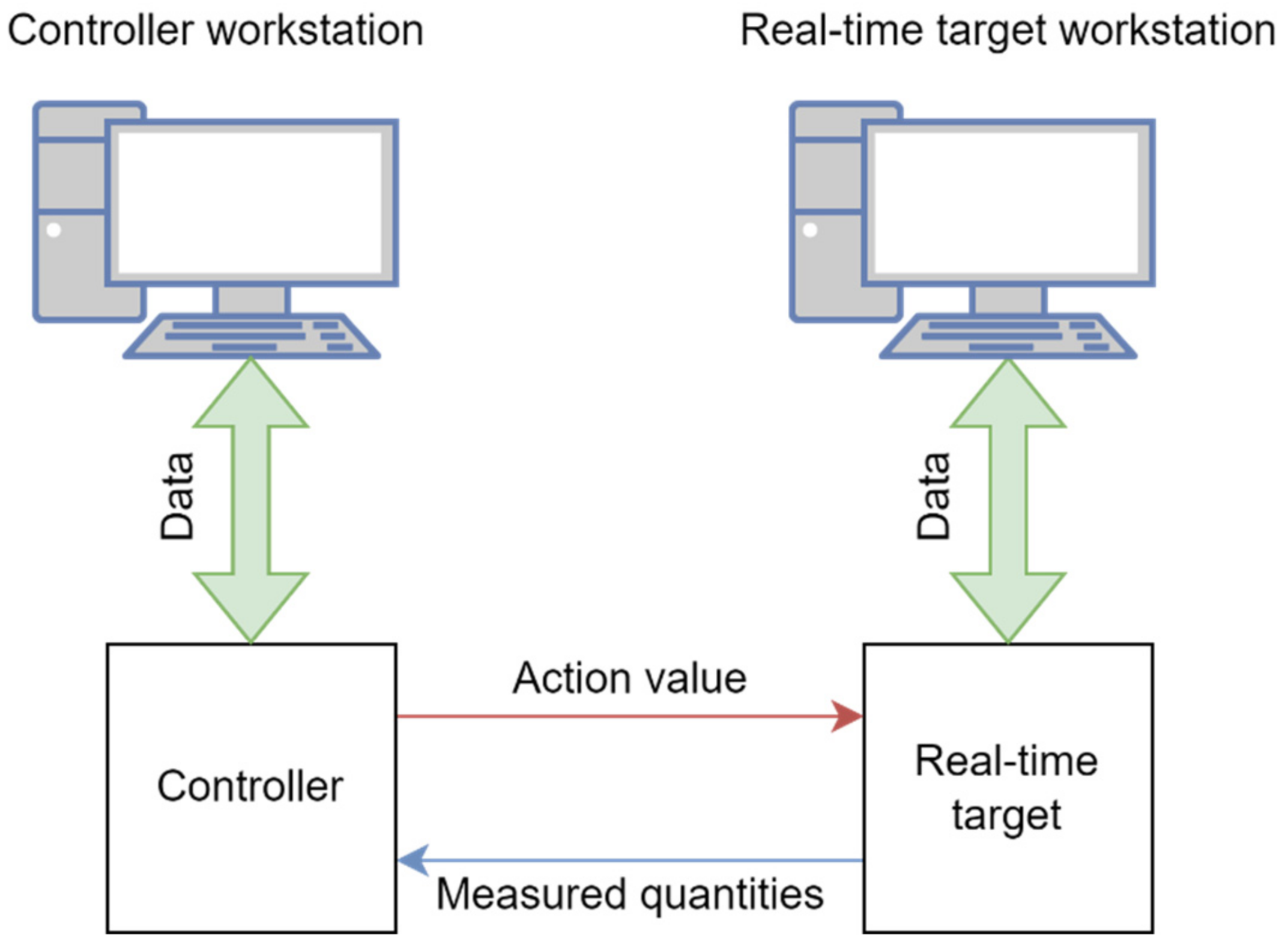
MiL is performed in the simulation environment (i.e., Matlab/Simulink) where both the controller and the plant are mathematical models. SiL is performed in the simulation environment as well, but the controller is implemented as a code (i.e., C/C++) that is going to be implemented in the controller. PiL performs a simulation where the controller code is implemented on a development prototyping board and is connected through the I/O interface with the computer that simulates the plant. The last technique to be mentioned is HiL (
Figure 2), which works on a similar principle to PiL, with the difference that the controller is run in real-time on the intended hardware and the plant simulation model runs on the real-time target. The HiL tests can also include safety functions.
One of the most significant advantages of the model-based design approach is the automatic code generation [
12,
13]. Therefore, we had to choose a controller that is powerful enough to perform our code in real-time and supports the conversion of our controller model from the Matlab/Simulink environment, to the form that is compatible with the selected controller. For this purpose, we have chosen the PLCnext controller, which meets the defined requirements [
14]. The programming code can also be created in classical PLC languages according to the IEC 61131-3 or in C#, C/C++, etc. The code created by both approaches can be combined and merged into the complete control system. PLCnext can also run an HMI application for visualisation and control. Since PLCnext can run as a web server, the HMI application can be accessed through the standard web browser.
In this article, we are concerned with the transition from the design phase to the system integration phase and verification of the designed control strategy for the Stewart platform. In the first part, we describe the Stewart platform parallel mechanism. Then we present the multibody simulation model of the Stewart platform, the designed feedback control loop and the results of the MiL simulation. In the next part, we present the application of the HiL simulation technique, where the PLCnext is tested as the desired controller of the plant. The results of the HiL simulation are then compared with those of the MiL simulation. The last part also discusses the actual and potential benefits of this approach as well as the risks and obstacles that are bound to this development methodology in relation to our case.
2. Stewart Platform
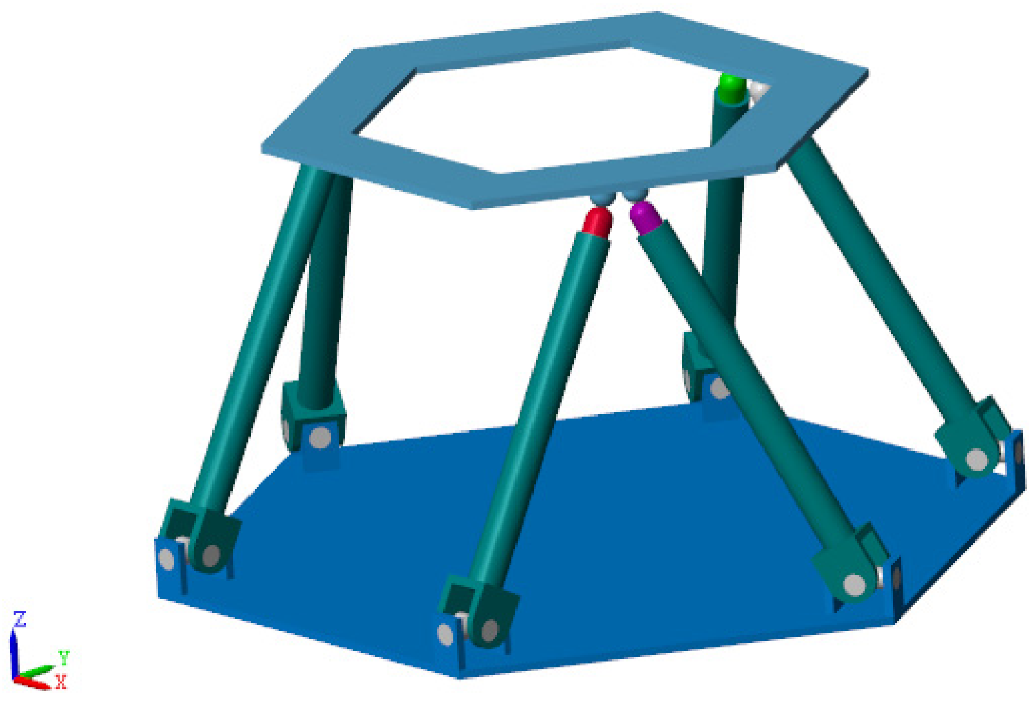
The Stewart platform (
Figure 3) is a parallel manipulator with six degrees of freedom [
15]. Its advantages are mainly its positioning precision, stiffness, and high power-to-density ratio. Its disadvantage is its relatively small workspace [
16,
17,
18]. Application of the Stewart platform can range from vibration isolation, motion simulators, to stabilization of a load, and more [
19,
20]. The Stewart platform consists of a base plate, six extensible legs, six upper and lower joint pairs, and a moving plate. The base plate is attached to the ground. The upper and lower joint pairs are formed by spherical and universal joints. The position and orientation of the moving plate depend on the extension of each extensible leg, which is represented by a linear actuator, which consists of a linear actuator body and a piston rod. The resulting trajectory of the moving plate is thus given by a synchronized motion of the actuators. The calculation of the required piston rod extension is done with the use of inverse kinematics [
21,
22].
As shown in
Figure 3, there is a base coordinate system
Obxbybzb fixed to the centre of the base plate. The lower joint position is given by
Bkb. The second coordinate system
Opxpypzp is fixed to the moving plate. The upper joint position is given by
Akp. The linear actuator body and the piston rod are related by a cylindrical joint. The linear actuator body is attached by the universal joint to the base plate. The piston rod is attached by the spherical joint to the moving plate. The position of the moving plate is given by (1). The orientation of the moving plate is given by roll
φ, pitch
θ and yaw
Ψ angles of the moving plate coordinate system with respect to the base coordinate system. The position and orientation of the moving plate is thus given by (2).
To calculate the leg length required to reach the desired
q, we need to use inverse kinematics (3). In this article, we will differentiate between desired position and orientation of the moving plate
qw and an actual position and orientation of the moving plate
qy. Based on the structure of the Stewart platform given by the vectors of upper and lower joint position
akp and
bkb, and the desired position and orientation, we can calculate the leg vector
lkb.
R is a rotation matrix.
C and
S represent
cos and
sin functions. The leg length is then obtained from (5). The leg length consists of
hk, which is a fixed length of the linear actuator body and
yk, which represents the piston rod extension. The piston rod extension
yk is controlled by the Stewart platform control system. The piston rod extension is given by a distance of the piston rod reference frame with respect to the linear actuator body reference frame as is described in
Section 3. Note that these calculations do not consider limitations such as minimum and maximum length of the extensible legs, as well as minimum and maximum joint angles, collisions of the bodies and singularity configurations. All these factors determine the workspace of the Stewart platform and should be checked on [
23].
3. Model-in-the-Loop (MiL) Simulation of the Stewart Platform
Since the development of the Stewart platform is done according to the V-Cycle, it has been supported with modelling and simulation tools, and therefore the multibody simulation model of the Stewart platform has been created. There are several methods available to build multibody simulation models of the Stewart platform.
The first one is to develop multibody simulation model with Newton-Euler, Lagrange or virtual work principle approach [
24,
25,
26]; these approaches are demanding, and it is hard to implement such models in the HiL simulation. Another approach is to develop the multibody simulation model with the use of software such as MSC Adams [
27], Matlab/Simulink [
28], etc.
In this paper, the presented simulation model has been developed with Matlab/Simulink and a Simscape Multibody toolbox. The mentioned software allows us to build a multibody simulation model in the Simulink environment with the blocks representing reference frames, bodies, joints, etc. However, it also supports the workflow, where the multibody assembly is exported from CAD software and is imported into the Matlab/Simulink environment [
28,
29]. The following Stewart platform simulation model has been created with the latter mentioned approach.
In
Figure 4 is the 3D visualisation of the created multibody simulation model of the Stewart platform. Its structure is similar to one presented in
Figure 3, but it has specified physical properties now. The function of the extensible leg is performed by a linear actuator, and the upper and lower joints are spherical and universal joints, respectively. This 3D model is viewed in the Mechanics Explorer that allows one to investigate the performance of the simulation model visually.
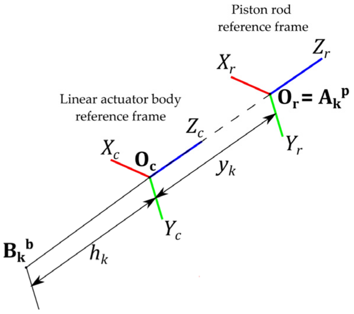
Each of the six linear actuators consists of a linear actuator body that is attached by a universal joint to the base and a piston rod that is attached to the moving plate by a spherical joint. Both the linear actuator body and the piston rod have reference frames attached to them. The linear actuator body has fixed coordinate frame
Ocxcyczc and the piston rod has fixed coordinate frame
Orxryrzr as is shown in
Figure 5. As mentioned in
Section 2, these two bodies are connected by a cylindrical joint and therefore the piston rod reference frame translates with respect to the linear actuator body reference frame along the
zc axis. As described in
Figure 5, the distance between the mentioned reference frames is
yk and is equivalent to the piston rod extension. The distance between the lower joint position
Bkb and the origin of the linear actuator body
Oc is equal to the fixed length of the linear actuator body
hk. A cylindrical joint block can be actuated and can have specified internal mechanics such as equilibrium position, spring stiffness, and a damping coefficient. Spring properties have not been used in our case and therefore this parameter is set to null.
The cylindrical joint operates in the forward dynamics mode, where the input is the acting force, and the resulting position of the piston rod is automatically computed. In this simulation model, the dynamics of the single cylindrical joint
k is described by the mass-damper model (6), defined by a damping coefficient
b and a mass
m, which are the same for each linear actuator. The acting force
Fak(t) is provided by the linear actuator and it is calculated in the feedback controller. The loading force
Flk(t) is acting on the linear actuator and varies with time as well. Its magnitude depends on the static configuration of the moving plate, as well as its dynamic movement and inertial properties.
The MiL scenario allows us to explore and verify the control strategies, the dynamic performance, and the workspace of the Stewart platform. It can also be used for SiL, PiL, and HiL simulations, which have already been mentioned before. However, in this article we present only MiL and HiL techniques.
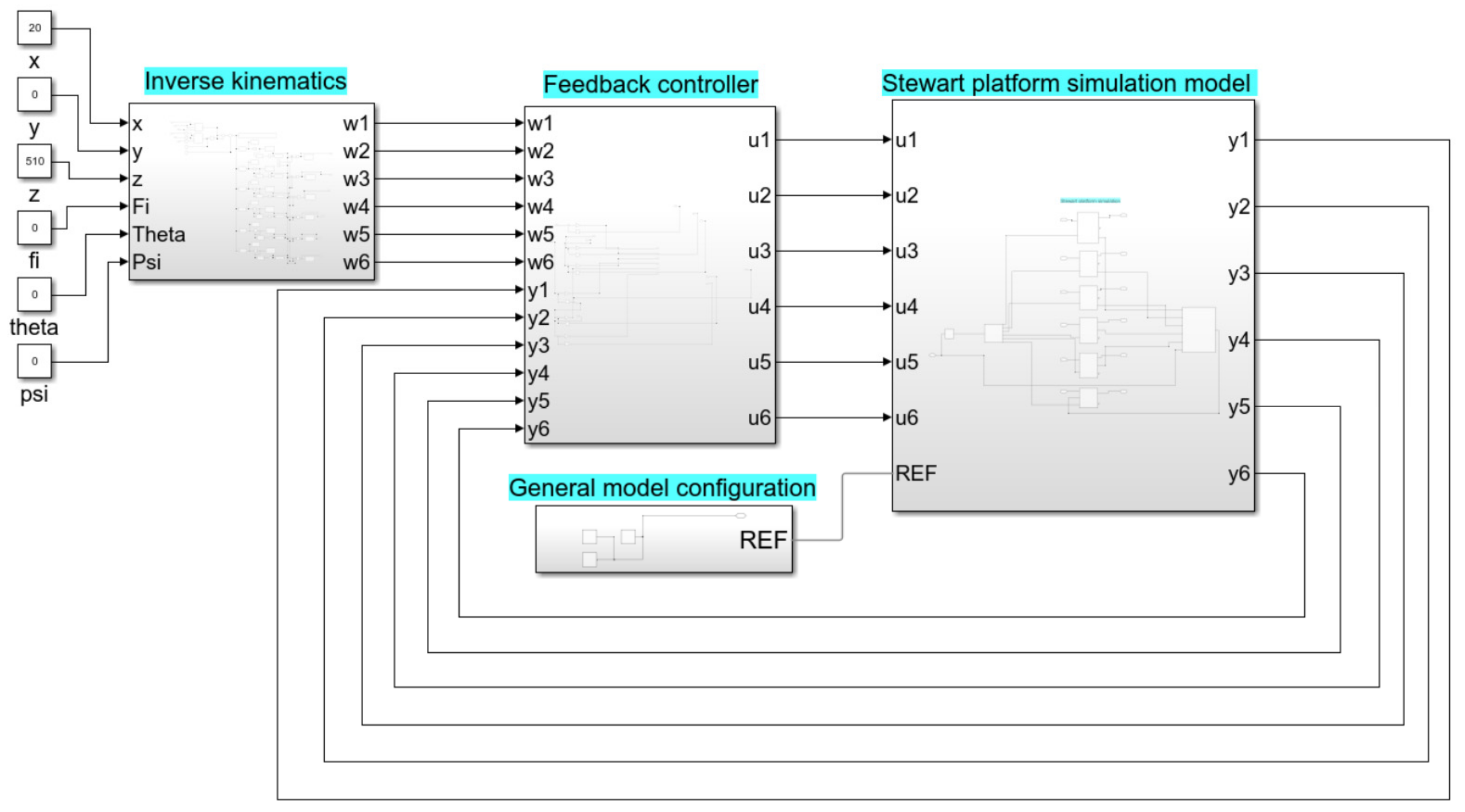
The multibody simulation model of the Stewart platform consists of a plant, a feedback controller, and an inverse kinematics block as shown in
Figure 6. The plant block in the Stewart platform simulation model has been mostly described in the previous text. The inputs
u of this block are six action values that represent the force that will be applied by each linear actuator. The six outputs
y carry information about the actual piston rod extension. These signals are used to control the position and orientation of the Stewart platform. Inside the plant block there is also an embedded block for a measurement of the position and orientation of the moving plate with respect to the world coordination system.
The inverse kinematics block shown in
Figure 6 calculates the desired piston rod extensions
[w1, w2, w3, w4, w5, w6]T based on the input
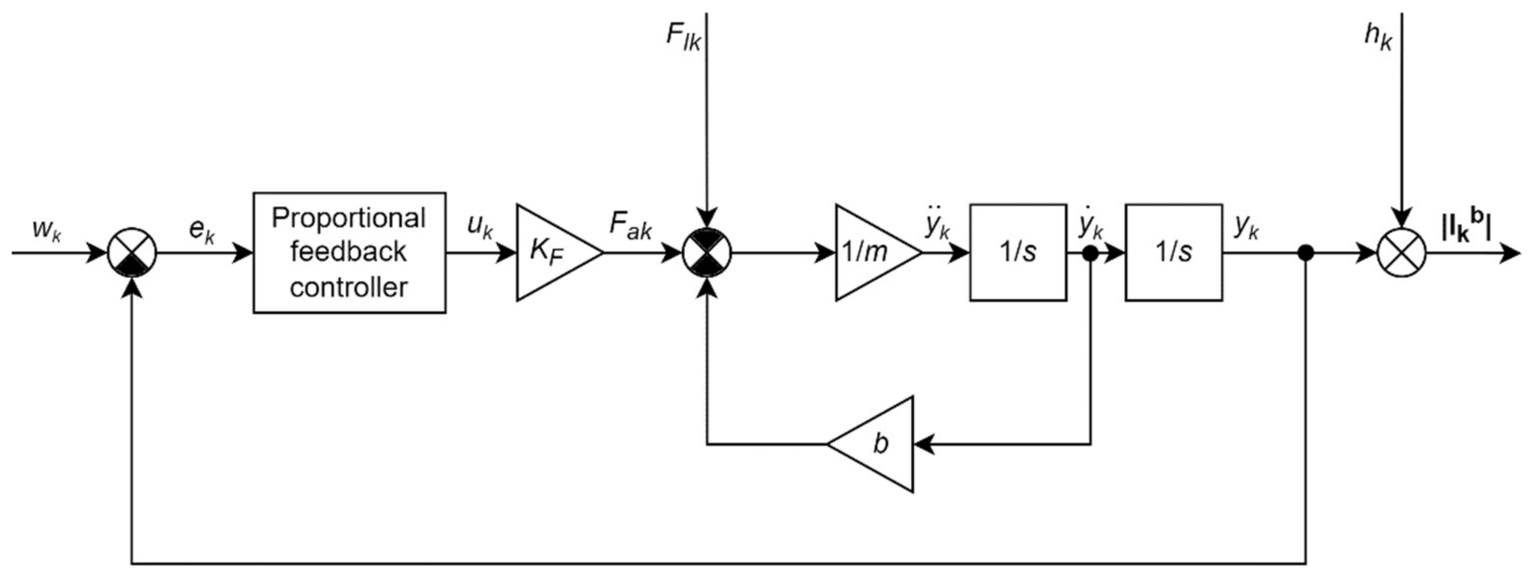
qw. The next block is the feedback controller that consists of six proportional feedback controllers. The feedback control loop for a single linear actuator is shown in
Figure 7. It consists of a proportional feedback controller and the single linear actuator plant. For the single linear actuator, the desired value
wk is calculated by the inverse kinematics block. The error value is given by
ek =
wk −
yk, where
yk is the actual piston rod extension. The action value
uk is equal to the acting force of the linear actuator
Fak. It should be noted that
wk varies in time if the moving plate is about to follow the desired trajectory. Gain
KF serves for a unit conversion of the action value
uk given in volts (V) to the acting force
Fak given in newtons (N).
Since our main focus during this experiment was not the best possible control performance, but rather an investigation of the model-based design approach, we designed a simple proportional feedback controller. For our system, it results in lower quality but functional control of the moving plate.
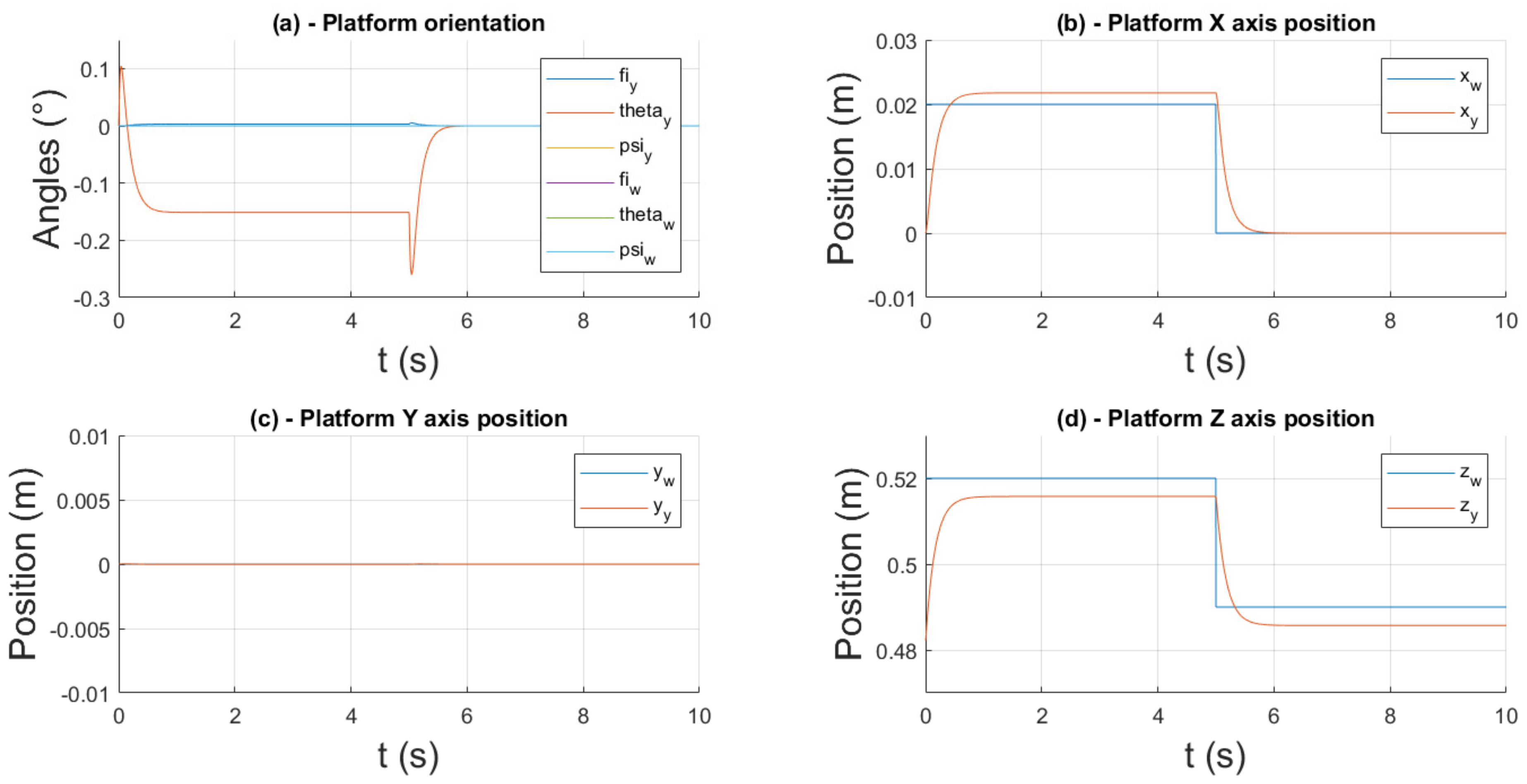
In the simulations, authors used the Runge–Kutta (ode4) solver with the fixed-step size 2 ms. In
Figure 8 can be seen transient responses of the moving plate for the step changes of the position of the Stewart platform. The initial desired position and orientation of the Stewart platform is
qw0 = [0, 0, 0.49, 0°, 0°, 0°]
T. The second desired position and orientation of the moving plate is
qw1 = [0.02, 0, 0.52, 0°, 0°, 0°]
T. From
Figure 8 can be seen that the moving plate moves first from
qw0 to
qw1 and then back to the
qw0. There is a visible deviation from the desired position and orientation of the moving plate. It must be noted that the desired angles
φw, θw, Ψw, which describe the orientation of the moving plate, are equal to 0°. As can be seen in
Figure 8, the deviation between desired and actual angles
φy,
Ψy is negligible. The deviation between desired and actual angle
θy is more prominent.
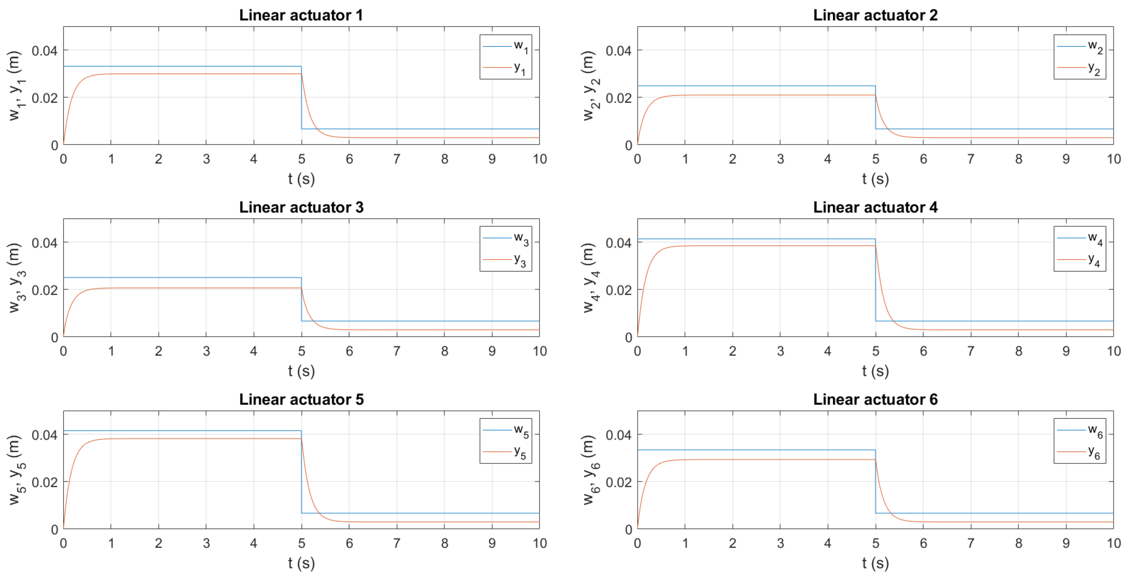
In
Figure 9, six transient responses of the piston rod extensions can be seen. The response times are sufficient, but due to the choice of the proportional controller there is a permanent control deviation that resulted in the error in position and orientation of the moving plate, as we can see in
Figure 8.
In
Figure 10, the acting forces
Fa that are equivalent to the action input
u, can be seen over time. It is visible that when the desired value changes the piston sharply accelerates and then decelerates until it reaches the steady state. Since bodies in the multibody simulation are subjected to gravitational forces, the steady state force of the linear actuators is non-null. It should also be noted that the applied force reaches both positive and negative values, which means that linear actuators are subjected to compressive and tensile loads.
In this section, we have described the simulation model of the Stewart platform and the MiL scenario.
Section 4 describes the Hardware-in-the-Loop experiment and compare its results to the results obtained in the MiL scenario.
4. Hardware-in-the-Loop (HiL) Simulation of the Stewart Platform
In this section, we present the HiL technique in the Stewart platform development procedure according to the model-based design approach. In this scenario, we can test and potentially validate the PLCnext controller for the Stewart platform control. In this case, the plant is generated as a code and uploaded to the real-time target dSPACE MicroLabBox (MLB). The inverse kinematics part of the control algorithm is generated as a code from the Matlab/Simulink environment as well and uploaded to the PLCnext as a subroutine. PLCnext consists of both generated Matlab/Simulink code and code programmed in its own programming environment PLCnext Engineer. PLCnext also allows running HMI for control and visualisation of the process. Since PLCnext has web server functionality, the HMI can be accessed through the web browser.
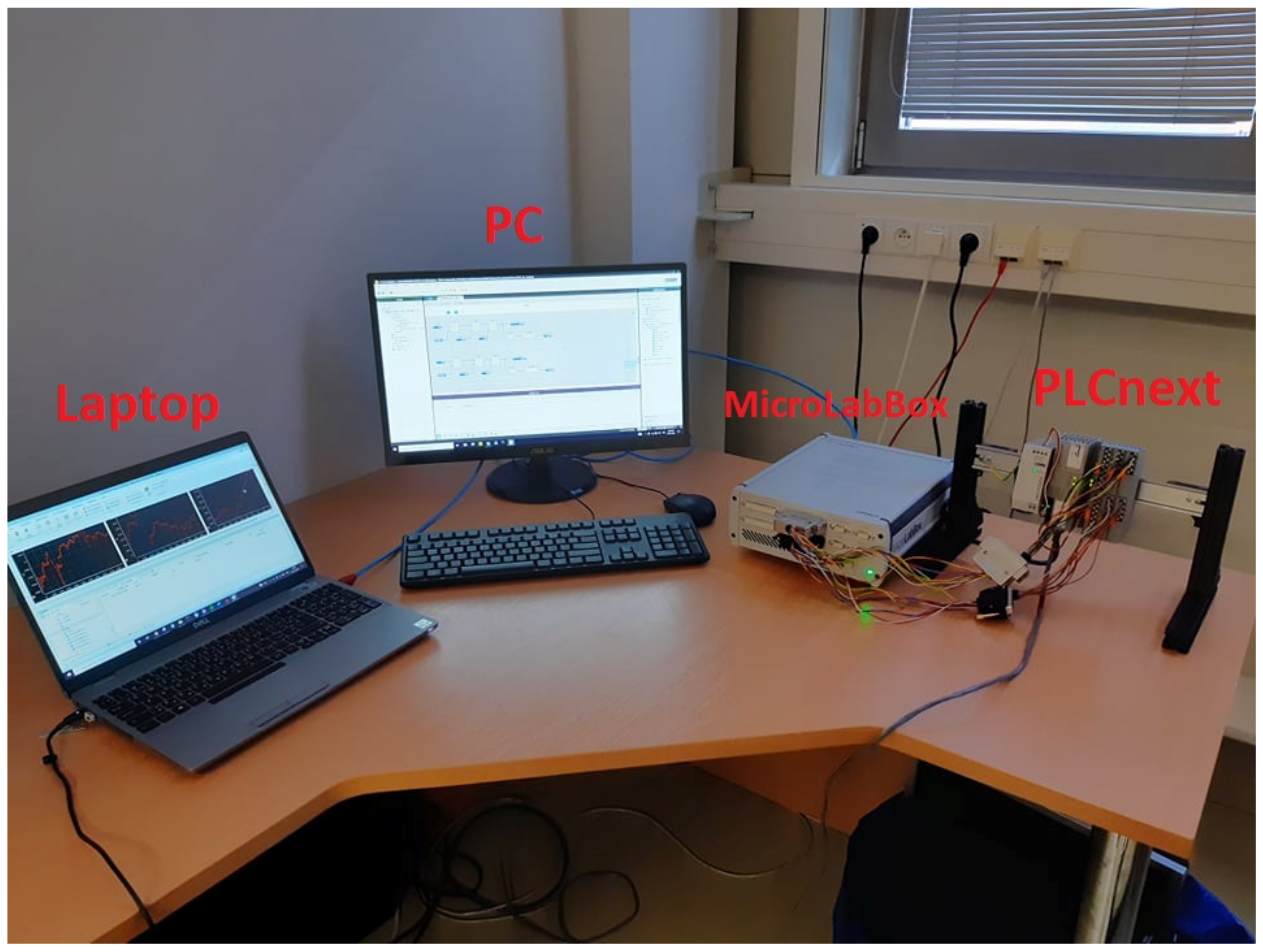
In
Figure 11 a workplace for the HiL simulation is shown. It consists of the PLCnext, the MLB, a PC, and a laptop. PLCnext and MLB are connected to each other through the I/O interface that consists of analog inputs and outputs operating in the range 0–10 V. PLCnext is also connected to the PC through Ethernet. This connection serves to upload the code to the controller and access the HMI, where an operator enters the desired position and orientation of the moving plate
qw. The MLB is also connected to the laptop via Ethernet. In addition to uploading the code to the real-time target, it also serves for visualising and data acquisition in the ControlDesk environment. The mentioned environment also allows the user to manipulate the parameters of the plant. The plant parameters have not been changed during this simulation experiment.
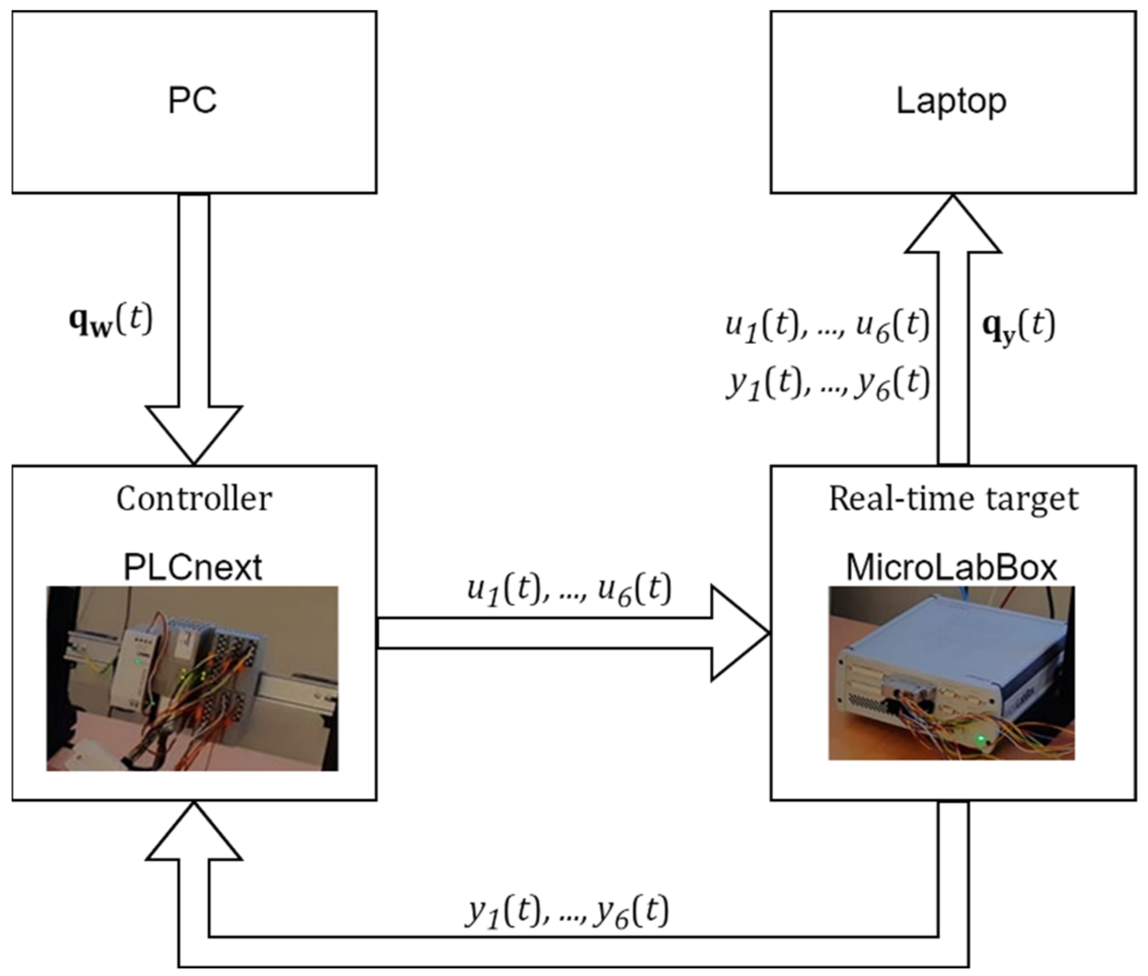
The HiL simulation scheme is also described by the diagram in
Figure 12. Where
qw is a vector carrying information about the desired position and orientation of the moving plate. The operator enters
qw values via the HMI interface on the PC. The controller PLCnext contains inverse kinematics and proportional feedback controller code and is based on the operator input and actual leg extension
y1, …, y6(
t) calculates action values
u1, …, u6(
t) for each linear actuator, which are part of the simulated plant in the real-time target MicroLabBox. MLB is connected with the laptop. As mentioned in the previous paragraph, the ControlDesk environment, which is running on the laptop, can be used for the data acquisition and the visualisation of the action values, actual piston rod extensions and an actual position and orientation of the moving plate
qy.
Code generation allows us to seamlessly transit from the design phase to the system integration phase. This approach saves a significant amount of time that would otherwise be required if both real-time target and controller had to be coded manually. The main reason is that manual coding is prone to human errors and is also very technically demanding, especially in the case of the plant code. Moreover, PLC programming languages typically do not support tools for linear algebra (i.e., matrix operations), which would make implementing inverse kinematics challenging as well. With the described tools, we can test and validate the chosen controller in this early phase of development before the first prototype has been built, which can significantly reduce time and costs. Nevertheless, we must be sure that the fidelity of the simulated plant is accurate enough before we draw any important conclusions.
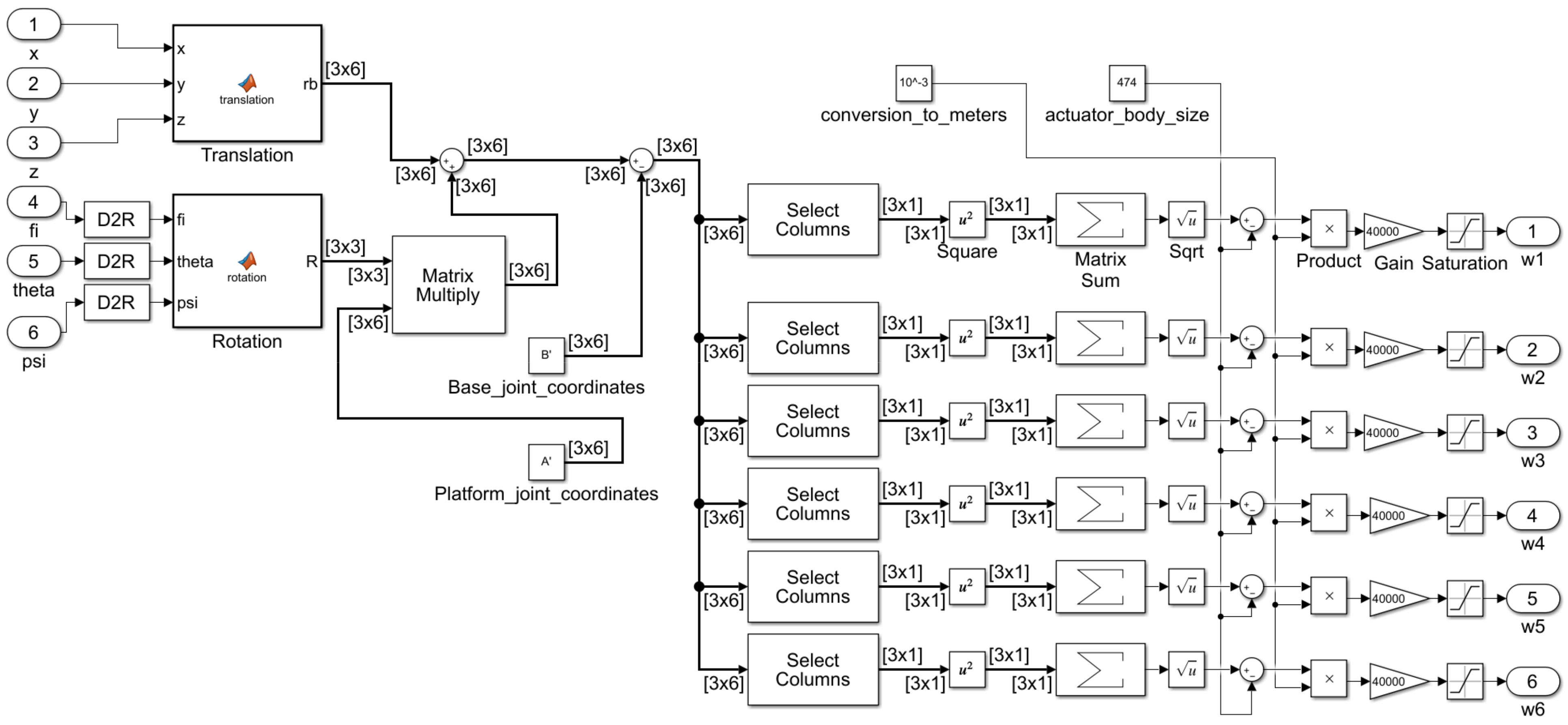
In
Figure 13 the inverse kinematics algorithm implemented in the Simulink environment can be seen. The implementation of the inverse kinematics is based on equations presented in
Section 2; however, they are adjusted for the Simulink implementation. The terms of the vector
qw are defined as inputs, and the calculated outputs
w1, …, w6 are the desired piston rod extensions. The block actuator body size shown in
Figure 13 is equal to the length of the linear actuator body
hk. The signal representing the piston rod extensions is scaled to the required range. There is also a saturation block that prevents the output signal from being of a higher magnitude than allowed. When we generate the code out of this model, we get a library block that can be used in the PLCnext code. Programming is done in PLCnext Engineer, which is a software platform for Phoenix Contact automation controllers. In this environment, we can use the generated library block and use it as a subroutine in PLCnext. We must specify the task to which it belongs to and assign the input and output variables. The inner structure of the inverse kinematics library cannot be investigated in this environment. Only its inputs and outputs are available. Generated libraries, therefore, act like a black box.
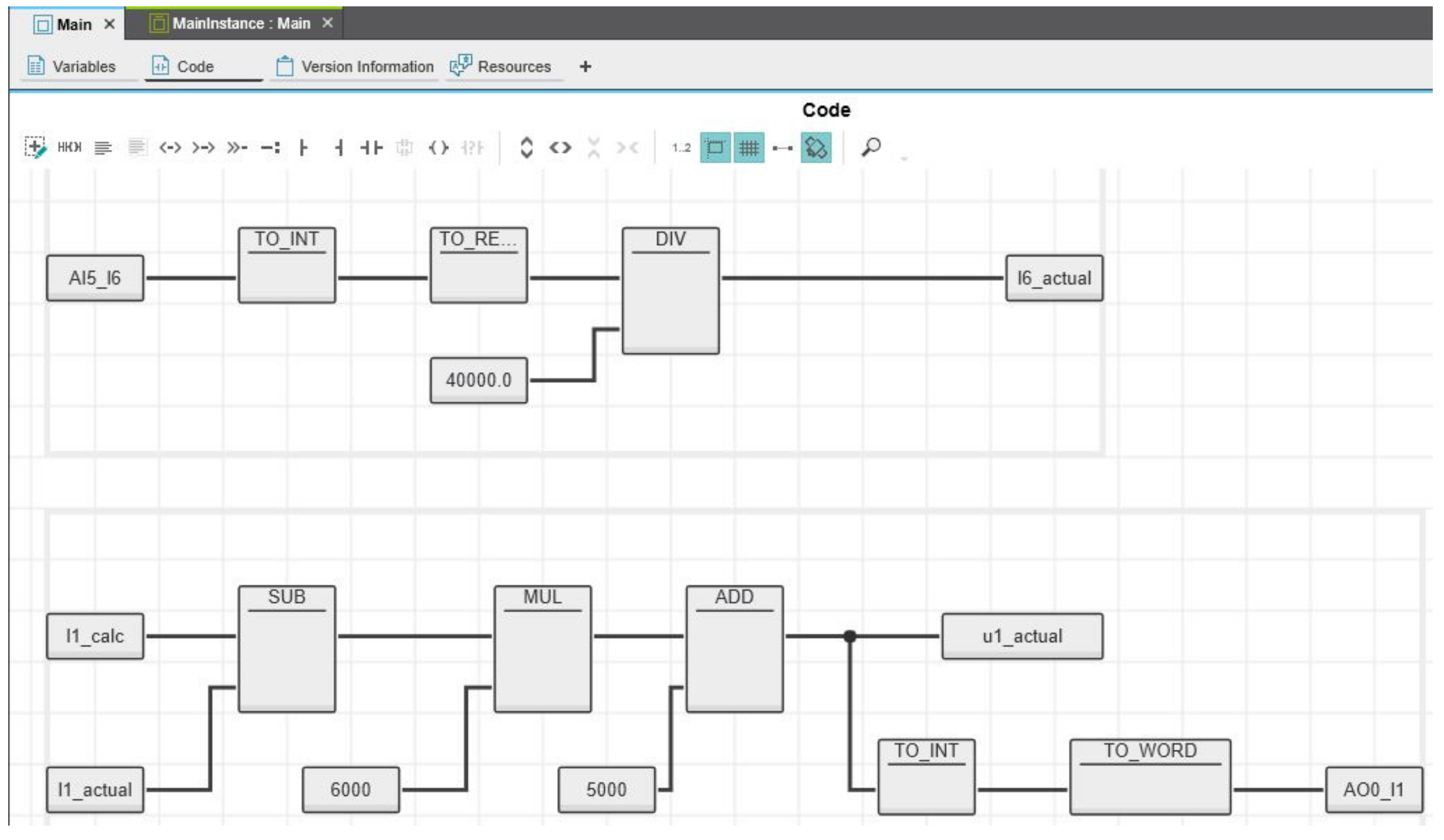
In the PLCnext Engineer, we have used the generated inverse kinematics block as a single subroutine. The feedback controller part has been coded directly in the new subroutine. The inverse kinematics subroutine for calculating desired leg lengths runs in the same cycle as the feedback controller subroutine with 1 ms time period. The snippet of the controller code is shown in
Figure 14.
In
Figure 14 the signal from analog input is shown to be processed and scaled. The same goes for the output signal. In
Figure 15 is a simple HMI interface that is used to define
qw. As mentioned before, HiL allows us to design and test graphical user interfaces and control systems higher in the control hierarchy even before the real prototype is built. In this configuration, it would also be possible to collect data from the simulation model and compare it to the data from the real Stewart platform, and thus this configuration could also be a significant part in the emerging research topic of the Digital twin [
30,
31,
32].
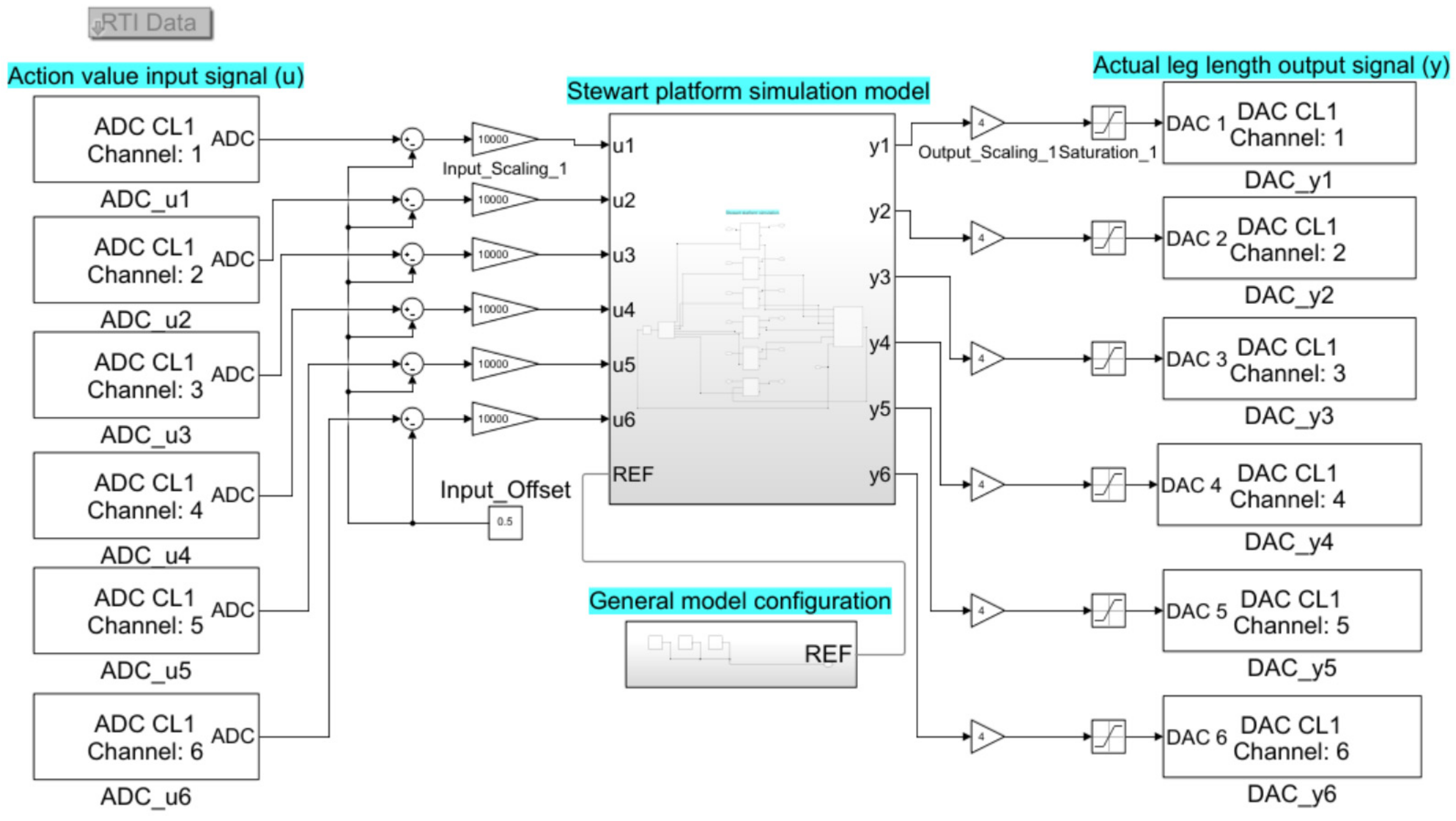
In the HiL plant simulation, authors used Runge–Kutta (ode4) solver with the fixed-step size 2 ms, as in the MiL scenario. In
Figure 16 is the HiL simulation model of the Stewart platform created in the Matlab/Simulink. This simulation model is adjusted for the real-time simulation in the MLB. The Stewart platform plant is the same as in the MiL scenario, only the blocks for the inverse kinematics and the feedback control have been adjusted and moved to the PLC controller. In the HiL simulation model, there are blocks for analog inputs that receive a signal that carries information of the action values
u. The blocks for the output signals, on the other hand, carry the information regarding the actual piston rod extension
y. Both input and output signals need to be scaled and processed accordingly.
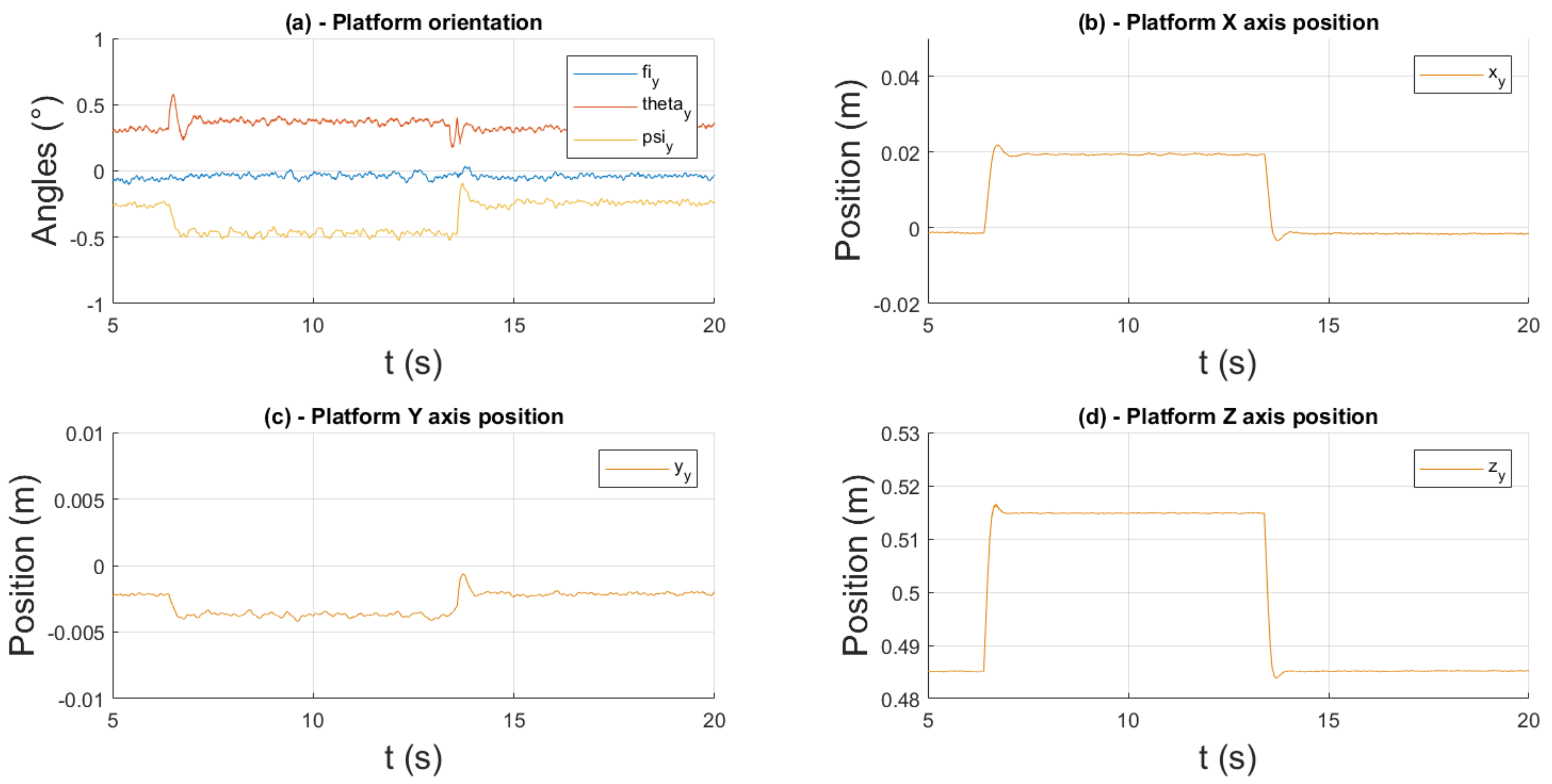
In
Figure 17 the transient responses of the moving plate for the step change of the position and orientation of the Stewart platform obtained during the HiL simulation can be seen. The initial and desired position and orientation
q0 and
q1 of the Stewart platform are the same as in the MiL scenario and the same operation has been performed as well but with the different timing. Since the desired value signal is not transferred to the MicroLabBox, we cannot display it in the same graph as
qy values.
The important conclusion from
Figure 17 is that analogically to the MiL scenario the error in linear actuator control results in the similar deviations of position and orientation of the moving plate. However, it must be noted that the steady state deviation in the platform orientation is more prominent and the transient responses are slightly oscillating.
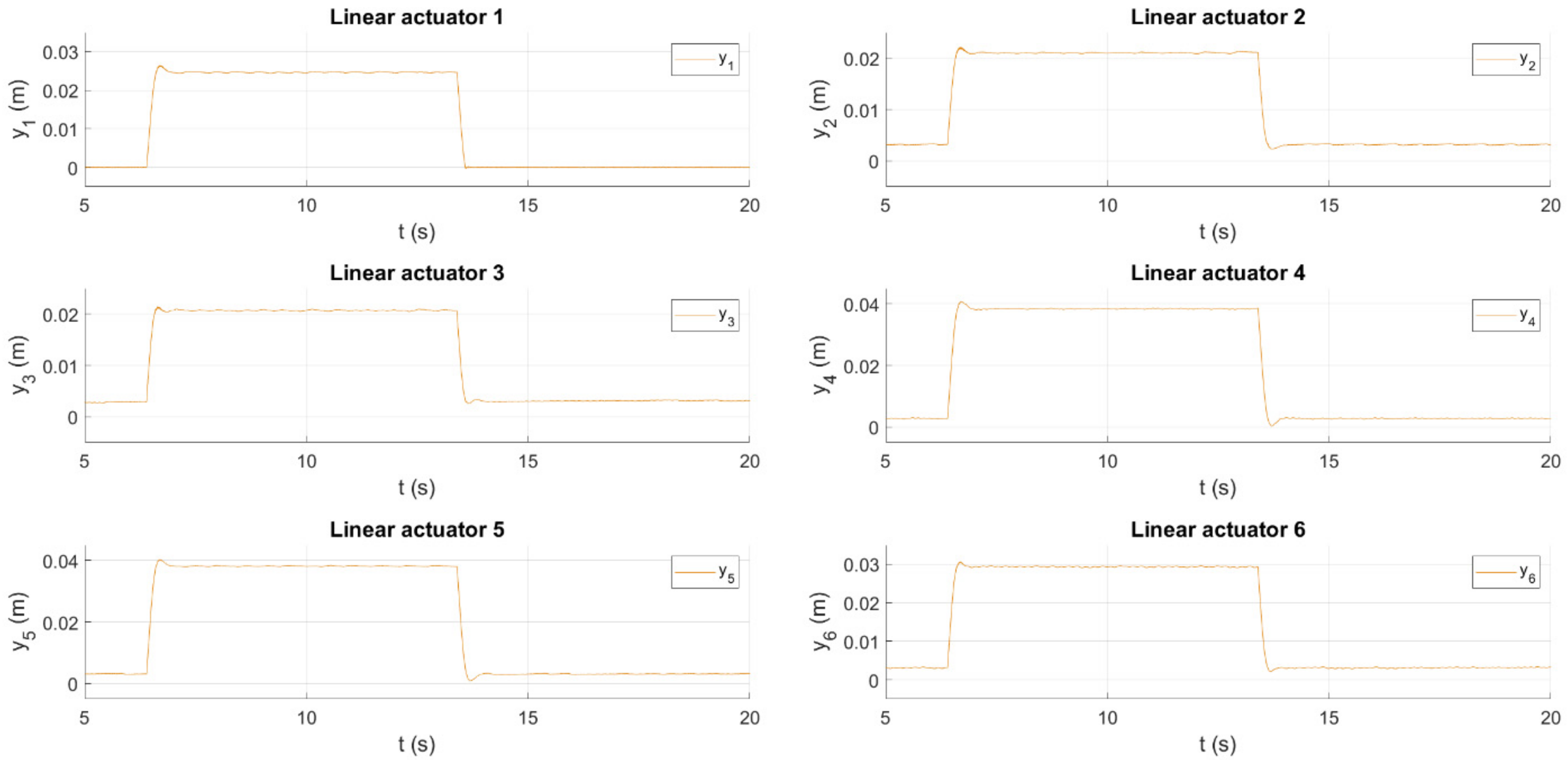
In
Figure 18 are transient responses of the piston rod extensions. Graphs show that transient responses are slightly oscillating, which is the reason the actual position and orientation of the moving plate is oscillating as well. The steady state values are comparable to the MiL scenario with the exception of the first linear actuator where a small error in magnitude is visible, which must result in an error in position and orientation of the moving plate. Authors assume this discrepancy is caused by one of the issues mentioned at the end of this chapter.
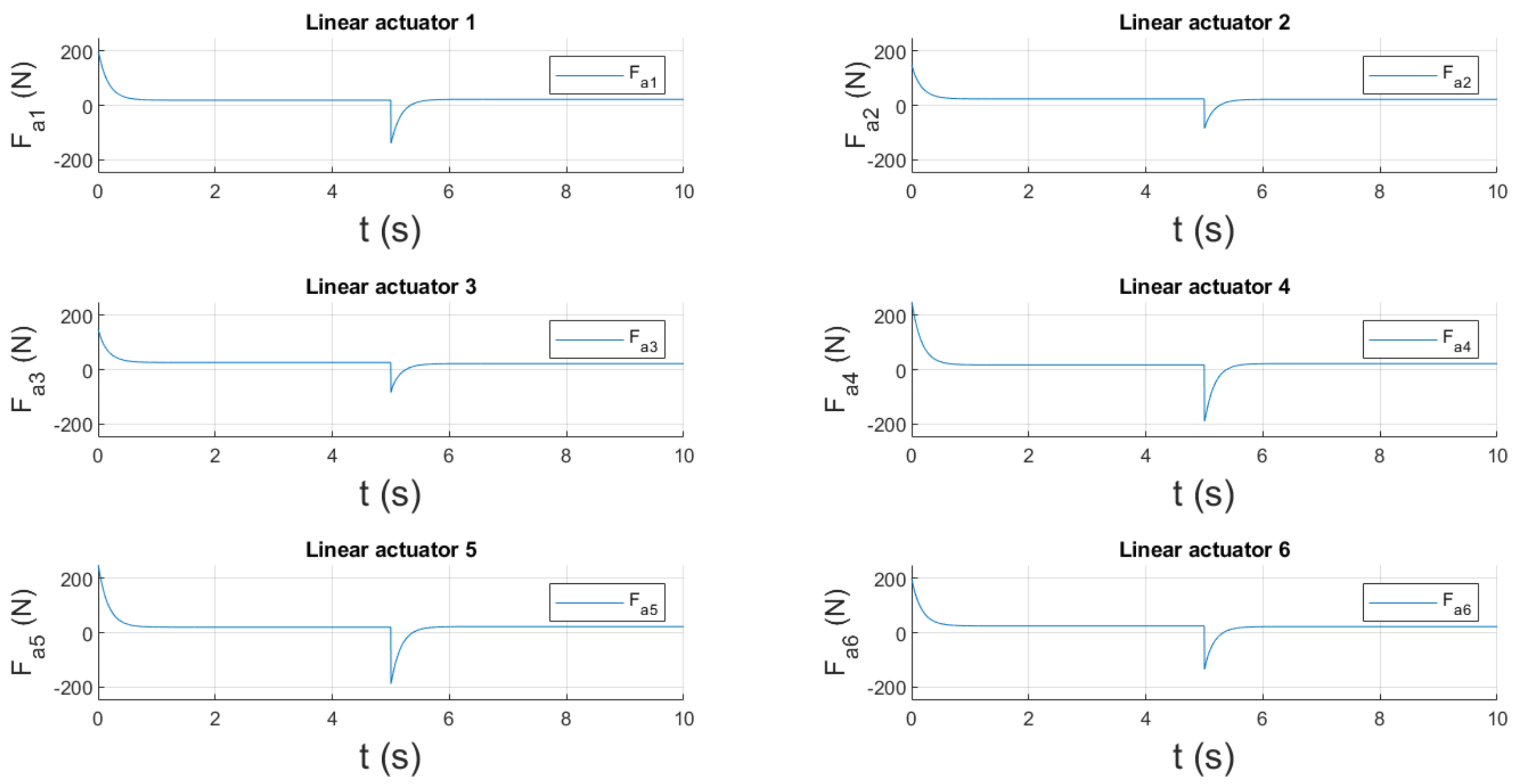
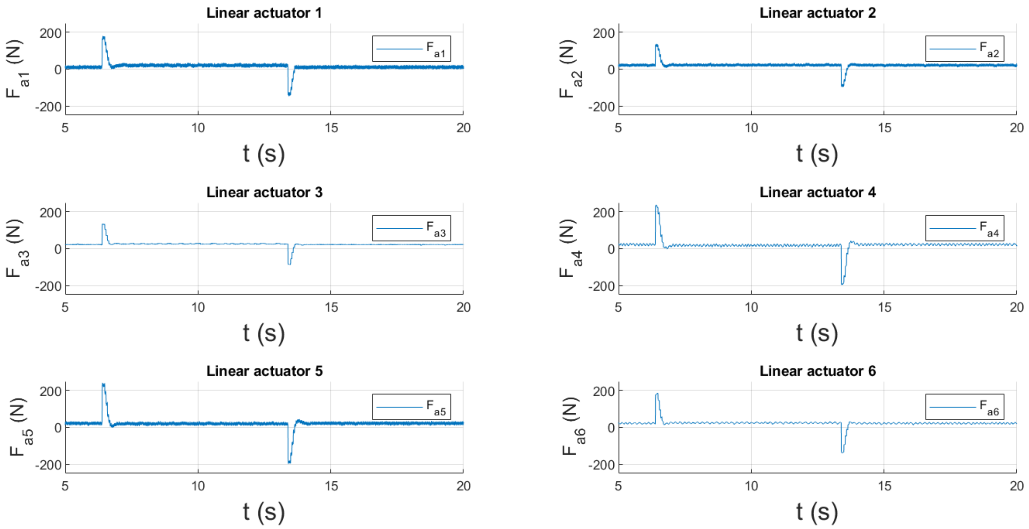
In
Figure 19 the acting forces
Fa of the linear actuators, that are equivalent to the action value inputs
u, are shown. It can be seen that the acting forces slightly oscillate and that the peak values and steady states are similar to the MiL simulation results.
Even though the obtained data cannot be directly compared to the MiL scenario, from the graphs it is obvious that the dynamics of the system is very similar. The main discrepancy in the MiL and HiL scenario is in the oscillation of the transient responses and the error in the magnitude of the first piston rod extension. These discrepancies can be caused by multiple issues such as different sampling periods of the controller and the simulated plant, connection of the real controller and the associated conversion of quantities from numerical format to voltage signal, quantization of signals during A/D and D/A conversions, rounding errors and also slight time delay. However, since most of the mentioned issues also occur during the control of the real system, the obtained results might represent the real control conditions. From this perspective, it is important that the control shows stability, required dynamics and accuracy which also depends on the type and parameters of the used controller.
The HiL technique allowed us to get acquainted with properties and behaviour of the Stewart platform in real-time scenario with an actual real controller design. It also allowed us to experiment with the system in the virtual environment and therefore we avoided the potential risk of destroying or damaging the real equipment. This scenario also possibly allows us to investigate the synchronization of the individual linear actuators which must be precise in high-precision Stewart platform applications.
5. Conclusions
In this paper we used methods for the mechatronics system development as described in the V-Cycle. We applied the model-based techniques Model-in-the-Loop and Hardware-in-the-Loop simulations in the case of the Stewart platform control strategy development. We discovered that the MiL method allowed us to get acquainted with the behaviour and properties of the system in the early stage of the design and we could also verify the controller part which was inverse kinematics and feedback control design.
In the next phase, we were able to translate smoothly from the design phase to the system integration phase, due to the fact that we were able to generate the inverse kinematics part of the designed controller code and used it as a subroutine in the real controller PLCnext. The feedback controller and HMI functions have then been coded manually and implemented in the single PLCnext programme with the inverse kinematic part. Since inverse kinematic calculations require matrix operations, which are usually not supported by any libraries in the PLCs, the code generation tools really accelerated this transition, and therefore we avoided coding the inverse kinematics in the standard PLC languages that would be error prone and cumbersome.
After obtaining the results from the HiL we found out that it slightly differs from the MiL scenario results. The main deviation was present in the slight oscillation of the transient response in the HiL results and the error in the magnitude in the piston rod extension of the first linear actuator. These discrepancies can be caused by multiple issues, mentioned in the article. From the perspective of the HiL simulation, it is important that the control shows stability, a required dynamics and accuracy, which also depend on the type and parameters of the used controller. The authors also must note, that during some of the scenarios of the HiL simulation experiments they ran into the numerical stability issues caused by the inability of the MicroLabBox to perform the calculations in the fixed step time. This issue did not occur in the MiL scenario. The authors therefore recommend that the readers use a more powerful real-time target than a MicroLabBox.
During the experiments, we discovered that the model-based approach is a strong technique, because it allowed us to explore the behaviour and properties of the system before the first prototype has been made in a virtual environment and therefore, we discovered potential issues early in the development phase that would result in reduced costs and time. That includes avoiding the potential for damaging and destroying the real equipment. However, it is fair to say that the employment of this approach is time-consuming in the initial stages, because development of the plant simulation model is demanding as well, and it is hard to verify the fidelity of the simulation model if the real prototype is nonexistent. Therefore, in the early design stages, it is required to approach the simulation results as critically as possible and it is necessary to continually improve precision of the used simulation model. Otherwise, false conclusions could be drawn, which would result in negative consequences in a later development phase.
In the HiL scenario, we are also able to test the developed functions of the controller and the higher control hierarchy as well. The obtained data can be processed and higher-level data processing algorithms can make decisions and conclusions based on them. Moreover, in case the developed simulation model of the plant accompanied the real product during the development cycle and has been previously verified and validated, it could possibly be used even after the development with the real product. The developed simulation model could be run in parallel with the real product as its digital twin. This could possibly add another value for the existing product and therefore it would return resources spent on the high-fidelity simulation model. In case of the Stewart platform, it could be used for the workspace investigation, trajectory planning, predictive maintenance, etc.


