SFINet: Shuffle–and–Fusion Interaction Networks for Wind Power Forecasting

Abstract

Wind energy is one of the most important renewable energy sources in the world. Accurate wind power prediction is of great significance for achieving reliable and economical power system operation and control. For this purpose, this paper is focused on wind power prediction based on a newly proposed shuffle–and–fusion interaction network (SFINet). First, a channel shuffle is employed to promote the interaction between timing features. Second, an attention block is proposed to fuse the original features and shuffled features to further increase the model’s sequential modeling capability. Finally, the developed shuffle–and–fusion interaction network model is tested using real-world wind power production data. Based on the results verified, it was proven that the proposed SFINet model can achieve better performance than other baseline methods, and it can be easily implemented in the field without requiring additional hardware and software.

1. Introduction

With the increasing global warming threats, the United Nations has called for the reduction of carbon dioxide emissions and hence set out the goals of reducing greenhouse gas emissions by 45 percent by 2030 and to net zero emissions by 2050 [1]. In line with the United Nations’ goals, the developed and most developing countries have started to take actions to develop realistic plans toward the reduction of carbon dioxide emissions. For instance, the Chinese government announced their goals to reach the peak of carbon dioxide emissions before 2030 and strive to achieve carbon neutrality before 2060 at the 75th session of the United Nations General Assembly (UNGA 75) in September 2020 [2]. In 2019, the total carbon dioxide emissions in China were estimated at 10.5 billion tons, of which the carbon emissions from energy consumption were about 9.8 billion tons, accounting for around 87% of the total emissions [3]. With rapid economic and social development, the transition to a green and low-carbon society is accelerated, and the transition of the country’s energy structure brooks no delay. Cleanliness is an important direction for carbon emission reduction in energy production. The way to accomplish the “dual carbon” task is to develop green and low-carbon renewable energy. During the 14th Five-Year Plan period, coal consumption in China will continue to decline. In the plan, it is forecasted that the installed capacity of renewable energy and nuclear power will reach 1200 GW by 2030, of which wind power will reach 500 GW in China [4].

As the installed capacity of wind power continues to grow and wind power is connected to the grid on a large scale, the overall grid performance is affected by the output power from wind farms due to the intermittency of wind [5]. In order to ensure the safety and stability of the operation of the power system, the power grid needs to prepare a sufficient spinning reserve capacity. However, the increase in the reserve capacity will increase the operating cost of wind power. Therefore, accurate wind power forecasting (WPF) is required for providing a basis to develop a grid dispatch schedule, and it also helps to greatly reduce the operating costs of wind farms and improve the competitiveness of wind energy in the overall energy market [6,7,8].

Historically, there have been different wind power forecasting (WPF) methods, which can be divided into four categories: physical, statistical, hybrid, and deep-learning methods. A summary report of these four categories of methods in terms of their features and limitations in application is given in [9]. The physical method is based on a mesoscale weather model or a numerical weather prediction system (NWP). NWP represents a variety of mathematical expression models of geographic and meteorological information [10,11]. Although this method has a good effect on short or medium-term forecasts of more than 3 h, it is difficult for it to collect all relevant geographic or meteorological data [12,13,14], so it has limitations in application. The physical forecasting method is generally used to select/determine new wind farms, but not for wind turbine power production prediction.

The statistical prediction method is based on the historical data collected by the SCADA system to establish a linear/non-linear relationship between relevant index data and power to predict the output power of a wind farm. Statistical prediction methods can be categorized as conventional statistical methods and those based on artificial neural networks (ANN). The conventional statistical methods have limitations in forecasting due to the demand for non-linear expression in wind power forecasting (WPF), while the methods based on artificial neural networks can effectively represent a large number of non-linear relationships and complex characteristics among wind speed, temperature, and other parameters in power generation. Therefore, statistical prediction methods based on ANN have become widely applied. Ref. [15] proposed a shallow model for wind speed prediction (WSF) based on artificial neural networks, which is more accurate than physical or traditional statistical methods.

The hybrid method integrates the physical and statistical models to improve forecast performance by preserving the advantages of each approach [16,17,18], but the hybrid models may not have the capability to achieve stable prediction, as their complex learning architecture may cause low efficiency in training and even underfitting [9].

With the development of deep learning techniques in recent years, and because wind power prediction possesses a natural time-series feature, some deep neural network (DNN)-based time series forecast methods have been developed and used for wind power estimation, such as the methods based on recurrent neural networks (RNNs) [19], long short-term memory (LSTM) [20], Transformer [21], temporal convolutional networks (TCNs) [22], sample convolution and interaction networks (SCINets) [23], etc. These form the deep learning-based method for wind power forecast. It is promising in terms of new model development for time series forecasting; however, none of the existing methods can claim to be perfect in time series prediction, which depends on the available data and data quality.

SCINet is a novel framework proposed by Liu et al. [23] very recently that has been applied to time series forecasting problems. It performs sample convolution and interaction at multiple resolutions for time-series modeling. Although good prediction results can be achieved by SCINet models, the SCINet framework has some shortcomings that affect the prediction performance, i.e., the prediction accuracy. One of the shortcomings is the strict binary tree structure taken in SCINet causing information blockage as the number of network levels increases. To address this issue, this present paper proposes a novel framework with a shuffle–and–fusion interaction network, named SFINet, to avoid the information blocking of SCINet sequence channels and develops an improved algorithm for wind power forecasting. The developed models based on SFINet have been proven effective to achieve the economic dispatch of energy production and reliable operation of the power system, providing an opportunity for reducing the operation costs of wind farms. The main contributions are as follows: (1) considering the sequence interaction modeling of time series tasks, we introduced the shuffle operation to increase the dependence between sequences; (2) in order to further promote interactive learning, we proposed feature fusion based on the time series attention mechanism; and (3) the developed models are applied to wind power forecasting using real wind power production data collected from a wind farm in China, verifying the outperformance of our models by comparing them with other baseline approaches.

2. Deep Learning-Based Method for Wind Turbine Operation and Power Forecasting

2.1. Channel Interleave Operation

To the best of our knowledge, the first real use of channel alternate operation was in IGCNets [24], and channel interleave in the form of shuffle was proposed in shufflenet [25], which aimed to break the information blockage between group convolutions. Subsequently, channel shufflenet has been widely utilized as a basic backbone network [26,27], with applications in semantic segmentation, Multi-Person Pose Estimation, Image Processing, and other tasks [28,29,30]. However, channel shufflenet is mostly used on the basis of grouped convolution and lightweight models. In this paper, we apply it to the construction of the sequence channels for time series forecasting to improve the interaction capabilities of different time series features.

2.2. Attention Mechanisms

Attention is essentially a tool to filter and focus important information from a large number of available processing resources, while ignoring non-important information [31,32]. It is usually combined with threshold functions, such as softmax and sigmoid, or sequential techniques [33,34]. In both computer vision and sequence tasks, it has shown superior performance [35,36]. In these applications, the attention mechanism usually acts on one or more top layers to further reshape the characteristics of the higher level. Attention mechanisms have provided a lot of benefits in many applications, e.g., image classification [37], object detection [38], multi-modal task [39], few-show learning [40], and machine translation [21].

The more common attentions are channel attention [37,41], spatial attention [37,42], temporal attention [43], and branch attention [44]. Channel attention adaptively recalibrates the weight of each channel and can be viewed as an object selection process, thus determining what to pay attention to. Hu et al. [41] introduced a lightweight attention operation with a Squeeze–and–Excitation block to model channel-wise relationships. Spatial attention can be seen as an adaptive spatial region selection mechanism for determining where to pay attention to. Dai et al. [42] proposed deformable convolutional networks (deformable ConvNets) to be invariant to geometric transformations, but they paid attention to the important regions in a different manner. Self attention [21] is also used as a spatial attention mechanism to capture global information. Temporal attention is a dynamic time-selection mechanism. Li et al. [43] proposed a global–local temporal representation (GLTR) to exploit multi-scale temporal cues in a video sequence. In a multi-branch structure, branch attention is used for branch selection. Reference [44] proposed an automatic selection operation called selective kernel (SK) convolution implemented using three operations: split, fuse, and select.

The above-mentioned attention methods are often combined in application. Chen et al. [45] dynamically modulated the sentence generation context in multi-layer feature maps using encoding channel attention and spatial attention. Reference [46] identified spatial saliency associated with image pixels and executed temporal intensity filtering and predictive coding to filter spatiotemporal redundancies from images.

On the basis of the above overview, we propose a feature fusion method based on time series channel attention, aiming to enhance the model’s long-term forecasting ability in wind power forecasting.

2.3. Deep Learning-Based Wind Power Forecasting

The wind speed and power indicators collected through the wind turbine SCADA system are all time series data. Time series forecasting can estimate their future development based on indicators or events. At the same time, there are complex nonlinear relationships among other indicator data related to power. From the previously published research works, it has been realized that deep learning-based time series forecasting has higher forecasting accuracy than the traditional methods [47], so the deep learning-based time series forecasting (TSF) method has been widely utilized.

The recurrent neural network (RNN)-based TSF method given in [48,49] compactly summarizes the past information in the internal memory used for prediction, where the memory state is recursively updated with new inputs at each time step, as shown in Figure 1a below. Ref. [50] proposed a long and short-term memory-based recurrent neural network (LSTM-RNN) to predict the wind power from 1 to 24 h. Transformer relies on the attention mechanism to model the global dependency of input and output, and breaks the non-parallelization problem of RNN-based methods, so it is gradually replacing the RNN model in almost all sequence modeling tasks. Therefore, various Transformer-based TSF methods were presented in [51], as shown in Figure 1b. The multi-head self-attention mechanism is used to extract the spatial correlation between wind farms [52]. Models based on convolutional neural networks (CNNs), such as temporal convolutional networks (TCNs), are also used in time series forecasting (TSF) [53,54]. The TCN uses a series of causal convolutional layers stacked to make full use of convolution. Parallel operation with efficient modeling of the dependency relationship between multiple sequence features is shown in Figure 1c. Long-term prediction of wind power with a mean absolute percentage error of 10% was carried out in [9] by using the temporal convolutional network (TCN).

Ref. [23] proposed a new neural network structure named SCINet, as shown in Figure 1d, specifically designed for time series forecasting, which lifts causal convolutional layers and the forced numbers of network input and output to be the same constraints of TCNs, and achieved very good performance in TSF tasks. To the best of our knowledge, however, SCINet has not been applied to the field of wind power forecasting (WPF). At the same time, the binary tree structure of SCINet causes information blockage as the number of network levels increases. For this reason, we propose shuffle–and–fusion interaction networks (SFINet) to overcome this issue.

3. SFINet: Shuffle–and–Fusion Interaction in Convolution Networks

As mentioned above, SCINet follows the strictly binary tree structure, and the time-series feature information will no longer have the opportunity for information interaction after passing through the parent node of the binary tree. Although there is an interactive learning operation in SCI-Block, it can fuse information between time-series, but this interactive process only exists at the node of the parent tree, which means that the subsequent layers of different depths can only come from the first interactive learning of the parent node for the most primitive timing input. As the number of tree layers deepens, this information will be transmitted more insignificantly. We think that this feature is very unfavorable for capturing the dependencies between long sequences.

We use Figure 2 to illustrate this feature of the original SCINet structure, where the most basic unit is SCI-Block, as shown in Figure 2a. SCI-Block contains interactive learning modules responsible for the interaction between two different timing features. The SCINet is composed of basic SCI-Blocks according to the strictly binary tree structure, as shown in Figure 2b, and the SCI-Block always averages the split input features in the timing dimension; finally, SCINet is stacked to form Stacked SCINet. We named the input feature of an SCI-Block as SSF (split-sequence features), then the input to the k-th SCI-Block of the l-th layer can be defined as SSF^{(l, k)}, where $\mathrm{l}=1,2,\dots ,\mathrm{L},\mathrm{and}\mathrm{k}=2^0,2^1,\dots ,2^{\mathrm{L}-1}$. Due to the average split characteristic in the timing dimension, for a timing sequence whose input length is known to be S, then $L\in \left[1,\mathrm{n}\right],\mathrm{and} 2^{\mathrm{n}}$ ≤ S.

Obviously, in the SCINet structure, SSF^{(l, k)} is with $\mathrm{l}>1,\mathrm{and}\mathrm{k}\in \left(1,2^{\mathrm{l}-1}\right)$. Only part of the output from the upper layer of the module will interact with other outputs in this layer. As shown in Figure 2b, each of SSF^{(3, 1)}, SSF^{(3, 2)}, SSF^{(3, 3)}, SSF^{(3, 4)} is input into the corresponding SCI-Block for further reasoning, and they are mutually isolated. Their interactive learning only exists in the first layer of SCI-Block. Hence, this property blocks information flow between sequential channels and weakens representation.

3.1. Shuffle Split-Sequence Features

If SCI-Block is allowed to obtain an input from different split-sequence features, the split-sequence features that characterize different time dimensions will obtain better interaction. Therefore, the shuffle operation was introduced on the basis of SCINet. Specifically, for the structural characteristics of SCINet, for each layer of input split-sequence features, the inputs are naturally presented in groups at each level. First, the channels of each group can be divided into sub-groups, and then different sub-groups can be evenly allocated to each group as the input to the next layer. This operation is a sequential operation, as shown in Figure 3a.

The above operations can be efficiently implemented through a channel shuffle operation, as shown in Figure 3b. Use $2^{\mathrm{l}}$ groups to form new sequence features, and its output channel has $2^{2\mathrm{l}}$ sub-groups. First, reshape the output channel size to$\left(2^{\mathrm{l}},2^{\mathrm{l}}\right)$, transposing and then flatten it back as the input of the next layer. Channel shuffling is also differentiable, which means that it can be embedded into network structures for end–to–end training. The shuffle operation makes it possible to build more powerful structures with sequential interactive learning.

On this basis, the shuffle operation was embedded in the SCINet structure, and therefore, the SFINet structure was designed as shown in Figure 3c. The shuffle operation acted on the output of all leaf nodes of all SCI-Blocks in each layer. There was only one shuffle operation in each layer, which had nothing to do with the number of SCI-Blocks in that layer.

3.2. Fusion with Channel Attention

Taking into account the natural law of features in timing, this paper does not directly use the feature $\overline{\mathrm{SSF}}$ after shuffle operation to replace the original SSF, but merges the two. Here, a simple method of adding corresponding positions was used to realize the fusion of the two parts; that is, to ensure the sequence relationship of the original SSF in time series and to ensure the communication of features in different slice groups.

Before feature fusion, the attention operation was further performed on $\overline{\mathrm{SSF}}$, which was completed by the attention block shown in Figure 4a.

First of all, in order to ensure that the features of each dimension on the timing channel are fully utilized and can participate in subsequent predictions, we propose squeezing global spatial information into a channel descriptor. Exploiting such information is prevalent in feature engineering work. We opted for the simplest. This was achieved by using global average pooling to generate channel-wise statistics. Formally, a statistic $\mathrm{z}\in {ℝ}^{\mathrm{c}}$was generated by shrinking $\overline{\mathrm{SSF}}$ through spatial dimensions W, where the c-th element of z is calculated by:

$${\mathrm{z}}_{\mathrm{c}}=F_g\left(\overline{\mathrm{SSF}}\right)=\frac{1}{W}{\displaystyle \sum }_{i=1}^w\overline{\mathrm{SSF}}\left(i\right)$$

(1)

To make use of the information aggregated in the squeeze operation, we followed it with a second operation that aims to fully capture channel-wise dependencies. We performed one-dimensional convolution again after Z, and the output was E. At the same time, it was to ensure that the characteristic channel output was the original length, and we finally used Sigmoid to activate E. Decoupling realizes the release of the dependency between different channels, and outputs of the final attention coefficient S = $\left[{\mathrm{s}}_1,{\mathrm{s}}_2,\dots ,{\mathrm{s}}_{\mathrm{c}}\right]$. The final output $\overline{\mathrm{X}}=\left[\overline{{\mathrm{x}}_1},\overline{{\mathrm{x}}_2},\dots ,\overline{{\mathrm{x}}_{\mathrm{c}}}\right]$ was obtained by rescaling the transformation output $\overline{\mathrm{SSF}}$ with the activation, such that the c-th element of $\overline{\mathrm{X}}$ was calculated by

$$\overline{{\mathrm{x}}_{\mathrm{c}}}={\mathrm{F}}_{\mathrm{scale}}\left({\mathrm{S}}_{\mathrm{c}},\overline{{\mathrm{SSF}}_{\mathrm{c}}}\right)={\mathrm{S}}_{\mathrm{c}}·\overline{{\mathrm{SSF}}_{\mathrm{c}}}$$

(2)

where${\mathrm{F}}_{\mathrm{scale}}\left({\mathrm{S}}_{\mathrm{c}},\overline{{\mathrm{SSF}}_{\mathrm{c}}}\right)$ refers to the channel-wise multiplication between the feature map $\overline{{\mathrm{SSF}}_{\mathrm{c}}}\in {ℝ}^{\mathrm{w}}$ and the scalar ${\mathrm{S}}_{\mathrm{c}}$.

Finally, we embedded the Attention Block into SCINet, as shown in Figure 4b; the output after the Attention Block will be added and fused with the original SSF and sent to the next layer of inference.

3.3. SFINet Architecture

After each layer of SCINet is the output, it is connected to the shuffle operation and attention block. Hence, a new network structure SFINet—the shuffle–and–fusion interaction network is proposed. This structure represents different timing information features. After passing through each layer, they will be shuffled and further processed at the attention block. After the above operations are completed, they will be fused with the previous features, and then enter the next layer of reasoning, thus breaking the information blockage in the original structure. After the above operations, not only the capture of short-term dependencies in timing is guaranteed, but also the ability to build long-term dependencies in timing is further improved.

It should be noted that, when level = 1, SFINet has the same structure as the original SCINet. Because the original input is directly connected to the output after a layer of reasoning, it does not go through the shuffle operation and attention block modules; however, in actual tasks, most tasks require a structure with larger than 2 levels.

4. Wind Power Forecast

This section provides a test of the proposed SFINet for wind power forecasting. Section 4.1 introduces the data sets included in this study. There were five data sets utilized: two of them were the collected real wind power data and three were the published data sets. Section 4.2 introduces detailed power prediction and other experimental settings. Section 4.3 shows the performance and usability of the proposed method, as well as the testing results. The effectiveness of SFINet was verified by comparing it with various other methods including SCINet.

4.1. Data Set Selection

We empirically perform the test of the established models using five data sets: two of them were collected from a wind farm and the other three were selected from the published benchmark data sets.

The data collected from a wind farm represent the operation data of two independent wind turbines, each with a rated power of 1.5 MW, for one year with a sampling frequency of once per 10 min, i.e., 10 min data. The two data sets were marked as WPm1 and WPm2, respectively. The data for each sampling point include 12 variables—see

Table 1. Illustration of the wind power data set including 12 variables.

Index	Name	1 January 2019 14:10	1 January 2019 14:20	1 January 2019 14:30	1 January 2019 14:40	1 January 2019 14:50	1 January 2019 15:00
1	Wind Speed (m/s)	3.37	3.00	*	3.40	3.13	3.46
2	Generator Output Power (KW)	0.0840	3.0268	*	21.6730	56.0637	104.1866
3	Pitch Angle (°)	75.81	27.10	*	40.70	−0.5	−0.5
4	Nacelle Position (°)	246.39	165.04	*	162.67	164.58	158.25
5	Vane Direction (°)	−76.09	−1.83	*	0.477	0.564	−2.687
6	Cumulative Power Generation (KWh)	7,856,887	7,856,887	7,856,887	7,856,887.5	7,856,894.0	7,856,904.3
7	Turbine Operation Mode	9.45	13.56	6	13.13	20	20
8	Generator Speed (rpm)	25.06	575.92	*	464.83	1098.54	1099.91
9	Temperature Outside Nacelle (°C)	21.60	21.60	*	21.60	21.30	20.80
10	Nacelle Y-direction Vibration Displacement (m)	−0.01098	−0.01108	*	−0.01330	−0.02163	−0.01448
11	Nacelle Z-direction Vibration Displacement (m)	−0.01098	−0.01108	*	−0.01331	−0.02163	−0.01448
12	Turbine Brake Level	27.625	17.085	*	20.57	0	0

Form description: * represents singular values.

below. These variables were most relevant to wind power generation, including the wind speed, generator output power, pitch angle, nacelle position (or yaw angle), wind direction (vane direction), etc. These variables were selected by referring to the previously published research articles for wind power forecast and through discussions with the wind farm operation manager and engineers. There were two wind turbine operation modes: Mode 1 was marked as 20 when there was power output to the grid and Mode 2 was marked as 6 when there was no power output or the wind turbine stopped running. Other values represent the wind turbine running in a transition status between the two operation modes. The value was calculated based on the time length when it was running in Mode 1 and the time length when it was running in Mode 2 in a 10 min time step. Similarly, there were two wind turbine braking modes: Under braking and no braking. When it was under braking, the variable Turbine Brake Level was assigned a value of 51, whereas it was given 0 if there was no braking. Other values assigned to this variable represent the braking is in a transition status between the two braking modes. The value was calculated based on the time length when it was in braking mode and the time length when there was no braking. Each value was calculated in average on a 10 min time step.

The ratio of the training data set to the validation set and the test set was 5:2:3. See

Table 2. The overall information of the 5 datasets.

Datasets	WPm1	WPm2	ETTh1	ETTh2	ETTm1
Variants	12	12	7	7	7
Total time steps	52,710	52,710	17,420	17,420	69,680
Time increment	10 min	10 min	1 h	1 h	15 min
Start time	1 January 2020	1 January 2020	1 July 2016	1 July 2016	1 July 2016
End time	31 December 2020	31 December 2020	26 June 2018	26 June 2018	26 June 2018
Task type	Multi-step	Multi-step	Multi-step	Multi-step	Multi-step
Data partition	5:2:3		3:1:1

for detailed information. These two data sets were used to verify the effectiveness of the proposed method in wind power forecasting.

Electricity Transformer Temperature (ETT) data were collected and used in [55]. The ETT data cover 2 years’ data collected from two separate counties in China. They were split into two data sets marked as ETTh1 and ETTh2, respectively, with a sampling frequency of once per hour. The ETTm1 data set was 15 min data, i.e., the sampling frequency was once per 15 min. Each data point consisted of the target value of “oil temperature” (°C) and six power load features—see

Table 3. Illustration of the ETT data set including 7 variables.

Index	Name	1 April 2018 0:00	1 April 2018 0:15	1 April 2018 0:30	1 April 2018 0:45	1 April 2018 1:00	1 April 2018 1:15
1	High Useful Load	17.281	16.075	16.946	15.606	13.932	17.281
2	High Useless Load	7.301	6.966	8.506	6.765	5.425	7.301
3	Middle Useful Load	12.793	12.153	12.757	11.833	9.559	12.864
4	Middle Useless Load	5.437	4.691	6.148	4.762	3.873	5.472
5	Low Useful Load	4.356	4.264	4.264	4.203	4.295	4.295
6	Low Useless Load	1.127	1.005	1.066	1.005	1.097	1.066
7	Oil Temperature	9.004	9.215	9.286	9.215	9.215	9.075

below. The ratio of the training data set to the validation set and the test set was 3:1:1. See Table 2 for detailed information. The ETT data sets were used to demonstrate the general validity of the proposed method.

4.2. Experiment Implementation

In order to evaluate the performance of the proposed method in different aspects, a variety of tasks were defined based on the wind power data set, including prediction tasks of different horizons and univariate or multivariate predictions.

In terms of horizon, similar to ETT data, in the case of a fixed sampling time, different output sequence lengths characterized different prediction times and also showed the difficulty of the task. The prediction lengths of WPh1 and WPh2 were divided into 6, 12, 24, and 48, and the corresponding prediction times were 1 h, 2 h, 4 h, and 8 h. In terms of variables, two forms of multivariate and univariate were used for evaluation. Univariate prediction takes the value of the generated wind power per second (A1gr Gen Power for Process_1sec), and multivariate prediction takes the values from all variables.

For ETT data, the prediction lengths of ETTh1 and ETTh2 were 24, 48, 96, 288, and 720, respectively, and the corresponding prediction time lengths were 24 h, 48 h, 96 h, 288 h, and 720 h. The predicted lengths of ETTm1 were 24, 48, 96, 288, and 672, corresponding to the predicted times of 6 h, 12 h, 24 h, 72 h, and 168 h, respectively. Univariate prediction takes the value of oil temperature, and multivariate prediction takes the values from all variables.

(1)

Evaluation index

The Mean Absolute Error (MAE) and Weighted Mean Absolute Percentage Error (WMAPE) were used as evaluation criteria. Because some variables in the task may have had negative values (the data sets in the format as Table 1 and Table 2), the optimized WMAPE was calculated as follows,

$$\mathrm{WMAPE}=\frac{{{\displaystyle \sum }}_{\mathrm{i}=0}^{\mathsf{\tau }}\left|{\overline{\mathrm{x}}}_{\mathrm{i}}-{\mathrm{x}}_{\mathrm{i}}\right|}{{{\displaystyle \sum }}_{\mathrm{i}=0}^{\mathsf{\tau }}\left|{\mathrm{x}}_{\mathrm{i}}\right|}$$

(3)

where τ is the total number of data points and ${\overline{\mathrm{x}}}_{\mathrm{i}}$ is the mean of the data in the sample.

The relative improvement of performance (RIP) with MAE and absolute improvement of performance (AIP) with WMAPE were used for comparison. They were calculated as follows:

$$\mathrm{RIP}=\frac{{\mathrm{MAE}}_{\mathrm{O}}-\mathrm{MAE}}{{\mathrm{MAE}}_{\mathrm{O}}},$$

(4)

$$\mathrm{AIP}={\mathrm{WMAPE}}_{\mathrm{o}}-\mathrm{WMAPE},$$

(5)

where MAE = $\frac{1}{\mathsf{\tau }}{\displaystyle \sum }_{\mathrm{i}=0}^{\mathsf{\tau }}\left|{\overline{\mathrm{x}}}_{\mathrm{i}}-{\mathrm{x}}_{\mathrm{i}}\right|,$ ${\mathrm{MAE}}_{\mathrm{o}}$and ${\mathrm{WMAPE}}_{\mathrm{o}}$ are obtained using other competitive methods for prediction, and MAE and WMAPE are obtained using the newly proposed method based on the SFINet model.

(2)

Data processing

In order to evaluate the performance of our proposed algorithm in wind turbine power prediction, we conducted experiments based on the proposed WP data sets and compared the prediction results with those given by the SCINet models. At the same time, in order to further verify the general applicability of the algorithm, we also verified the performance of the algorithm using the ETT data sets and compared it with other methods, including SCINet.

Our task does not specify the look-back windows corresponding to a certain prediction sequence horizon. In the wind power forecasting task, the original wind power data have singular values. In order to eliminate the singular values shown in Table 1, we chose to skip singular values when constructing the training, validation, and testing for different tasks. If there was a singular value in a pair, this piece of data was discarded. Therefore, in this way, for different tasks, the number of samples for training, validation, and testing were be produced, as shown in

Table 4. Wind power forecasting task setting and number of samples.

Task		WPm1				WPm2
Length	Horizon	6	12	24	48	6	12	24	48
	look-back	128	256	512	512	128	256	512	512
Number of samples	Training	24,150	22,810	20,248	20,032	24,400	23,418	21,388	21,220
	Validation	10,862	10,722	10,442	10,394	10,862	10,722	10,442	10,394
	Test	15,033	14,625	13,809	13,713	15,043	14,635	13,819	13,723

. Table 4 also shows the input data time length for a certain prediction length; for example, if the prediction length is for 6 h, the input data covers a time length of 128 h.

The singular value issue did not appear in the ETT data set, and these data could be used normally. In the ETT task, the settings are shown in

Table 5. ETT task setting and number of samples.

Task		ETTh1					ETTh2					ETTm1
Length	Horizon	24	48	168	336	720	24	48	168	336	720	24	48	96	288	672
	look-back	48	96	336	672	1440	48	96	336	672	1440	96	96	384	672	672
Number of samples	Training	8569	8497	8137	7633	7185	8569	8497	8137	7633	7185	34,441	34,417	34,081	33,601	33,217
	validation	2857	2833	2713	2545	2161	2857	2833	2713	2545	2161	11,497	11,473	11,425	11,233	10,849
	test	2857	2833	2713	2545	2161	2857	2833	2713	2545	2161	11,497	11,473	11,425	11,233	10,849

.

All data were normalized. In terms of the loss function and optimizer, we followed the same settings for the SCINet model given in [23].

(1)

Hardware platform

Training GPU: Single Nvidia 3080Ti 16 GB.

CPU Intel(R) Xeon(R) CPU E5-2650 v4 @ 2.20 GHz.

Memory: 256 G.

4.3. Prediction Experiment and Result Analysis

(1)

Wind power forecasting

Applying SFINet to the wind power data sets, the forecasting performance obtained is shown in

Table 6. Forecasting results evaluated in MAE on wind power data sets.

Variable	Methods	WPm1				WPm2
		Horizon				Horizon
		6	12	24	48	6	12	24	48
Multivariate	SCINet	0.287	0.353	0.4359	0.487	0.277	0.3252	0.4161	0.4978
	SFINet	0.276	0.327	0.392	0.452	0.2709	0.3191	0.384	0.452
	RIP	3.83%	7.37%	10.07%	7.19%	2.20%	1.88%	7.71%	9.20%
Univariate	SCINet	0.2351	0.3059	0.4032	0.5071	0.2319	0.3028	0.4059	0.4978
	SFINet	0.2291	0.2912	0.379	0.4721	0.2241	0.2851	0.378	0.4733
	RIP	2.55%	4.81%	6.00%	6.90%	3.36%	5.85%	6.87%	4.92%

. It can be seen from Table 6 that the prediction results of the SFINet model proposed in this paper were generally better than those of the SCINet model. The evaluation criteria of MAE using the multivariate and univariate prediction results with the WPm1 data set were reduced by up to 10.07% and 6.90%, respectively; and up to 9.20 and 6.87%, respectively, for the WPm2 data set.

The forecast results evaluated using WMAPE are shown in

Table 7. Forecasting results evaluated in WMAPE on wind power data sets.

Variable	Methods	WPm1				WPm2
		Horizon				Horizon
		6	12	24	48	6	12	24	48
Multivariate	SCINet	31.24%	0.3814	49.95%	55.38%	30.06%	39.69%	53.52%	65.83%
	SFINet	30.69%	36.44%	44.16%	50.47%	29.08%	37.06%	48.91%	60.97%
	AIP	0.55%	1.70%	5.79%	4.91%	0.98%	2.63%	4.61%	4.86%
Univariate	SCINet	29.94%	38.88%	52.74%	66.37%	30.79%	39.16%	52.73%	65.32%
	SFINet	28.84%	37.32%	49.58%	61.44%	29.08%	37.06%	48.91%	60.97%
	AIP	1.10%	1.56%	3.16%	4.93%	1.71%	2.10%	3.82%	4.35%

. From the results given in Table 7, the superiority of the SFINet model algorithm was verified in univariate and multivariate wind turbine power prediction. The evaluation indices of WMAPE with the WPm1 data set were reduced by up to 5.79% using multivariate evaluation and 4.93% using univariate evaluation, and the WMAPE with the WPm2 data set were reduced by up to 4.86 and 4.35%, respectively. The performance improvement trend of the SFINet model under different horizon tasks was similar to the results using MAE metric.

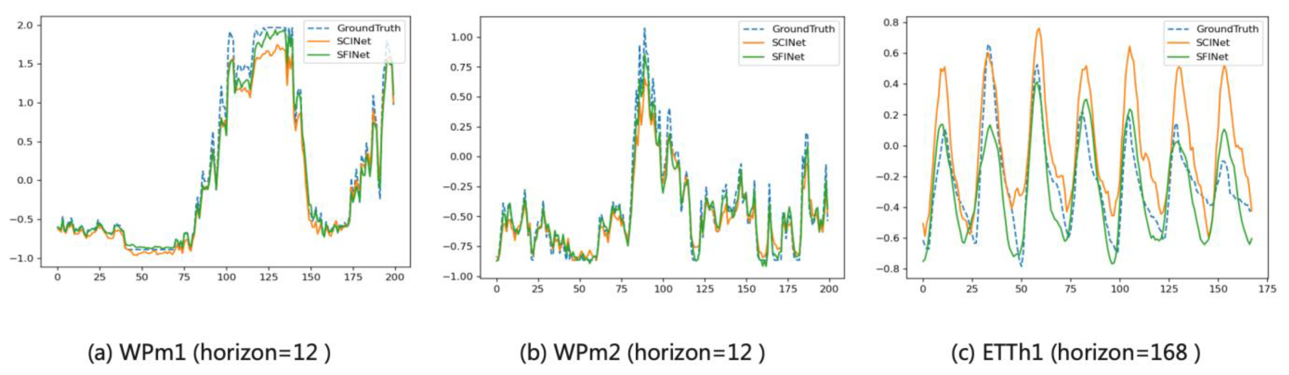
We then performed qualitative analysis of the prediction results using the wind power data set by selecting a piece of wind turbine power data for a sampling length of 200 in the WPh1 data set and WPh2 data set, as shown in Figure 5a,b. It can be seen that the forecasted wind power had the characteristics of large variation, violent fluctuations and no obvious laws to follow. The prediction result of the SFINet model could better fit the actual power curve. At the same time, at the peak and valley points of the power change, the prediction result of the SFINet model was generally better than that of the SCINet model (see also Figure 5c) by using the published data set.

(2)

Generalization study

The ETT data set given in [55] were used to evaluate the performance of a time series forecasting task e.g., [23,55]. In this paper, we used the same dataset to evaluate the performance of time series forecasting by different approaches, and the results of multivariate and univariate prediction are shown in

Table 8. Forecasting results evaluated by MAE on ETT datasets. The best results are in bold and the second-best results are underlined. RIP denotes the relative improvement of performance of the proposed method over the second-best results.

Variable	Methods	ETTh1					ETTh2					ETTm1
		Horizon					Horizon					Horizon
		24	48	168	336	720	24	48	168	336	720	24	48	96	288	672
Multivariate	Reformer	0.754	0.906	1.138	1.280	1.520	1.613	1.735	1.846	1.688	2.015	0.607	0.777	0.945	1.094	1.232
	LSTMa	0.624	0.675	0.867	0.994	1.322	0.813	1.221	1.674	1.549	1.788	0.629	0.939	0.913	1.124	1.555
	LogTrans	0.604	0.757	0.846	0.952	1.291	0.750	1.034	1.681	1.763	1.552	0.412	0.583	0.792	1.320	1.461
	Informer	0.549	0.625	0.752	0.873	0.896	0.665	1.001	1.515	1.340	1.473	0.369	0.503	0.614	0.786	0.926
	TCN	0.549	0.529	0.617	0.682	0.778	0.478	0.615	1.266	1.312	1.276	0.282	0.360	0.363	0.646	1.371
	SCINet	0.379	0.395	0.457	0.497	0.560	0.288	0.358	0.504	0.560	0.761	0.229	0.274	0.291	0.415	0.604
	SFINet	0.350	0.370	0.424	0.465	0.518	0.268	0.331	0.409	0.503	0.657	0.222	0.256	0.278	0.368	0.461
	RIP	7.65%	6.33%	7.22%	6.44%	7.50%	6.94%	7.54%	18.83%	10.18%	13.67%	3.06%	6.57%	4.47%	11.08%	23.68%
Univariate	Reformer	0.389	0.445	1.191	1.124	1.436	0.437	0.545	0.879	1.228	1.721	0.228	0.390	0.767	1.245	1.528
	LSTMa	0.275	0.330	0.763	1.820	3.253	0.381	0.462	1.068	2.543	4.664	0.290	0.305	0.396	0.574	1.174
	LogTrans	0.259	0.328	0.375	0.398	0.463	0.255	0.348	0.422	0.437	0.493	0.202	0.220	0.386	0.572	0.702
	Informer	0.247	0.319	0.346	0.387	0.435	0.240	0.314	0.389	0.417	0.431	0.137	0.203	0.372	0.554	0.644
	N-Beats	0.156	0.200	0.255	0.284	0.422	0.210	0.271	0.393	0.418	0.432	0.117	0.168	0.234	0.311	0.370
	SCINet	0.132	0.173	0.222	0.242	0.343	0.194	0.242	0.311	0.340	0.403	0.085	0.134	0.198	0.266	0.328
	SFINet	0.131	0.163	0.203	0.240	0.306	0.183	0.229	0.297	0.334	0.349	0.088	0.140	0.183	0.250	0.306
	RIP	0.76%	5.78%	5.58%	0.83%	10.79%	3.09%	5.37%	4.50%	1.76%	13.40%	1.14%	2.10%	7.58%	6.02%	6.71%

and

Table 9. Forecasting results evaluated by WMAPE on ETT datasets.

Variable	Methods	ETTh1					ETTh2					ETTm1
		Horizon					Horizon					Horizon
		24	48	168	336	720	24	48	168	336	720	24	48	96	288	672
Multivariate	SCINet	47.10%	49.92%	57.15%	61.57%	70.97%	20.83%	26.19%	36.79%	41.73%	56.88%	17.51%	19.98%	23.43%	30.45%	43.96%
	SFINet	44.22%	46.53%	52.88%	58.67%	64.84%	19.72%	23.82%	30.05%	37.41%	49.12%	16.38%	18.44%	20.48%	27.14%	34.00%
	AIP	2.88%	3.39%	4.27%	2.90%	6.13%	1.11%	2.37%	6.74%	4.32%	7.76%	1.13%	1.54%	2.95%	3.31%	9.96%
Univariate	SCINet	10.86%	16.62%	19.36%	22.36%	26.51%	18.66%	22.85%	29.93%	33.64%	45.33%	8.16%	13.20%	18.31%	23.96%	28.82%
	SFINet	9.82%	12.34%	15.09%	17.61%	22.18%	17.19%	20.65%	26.64%	32.83%	30.79%	7.73%	12.74%	16.60%	22.54%	27.35%
	AIP	1.04%	4.28%	4.27%	4.75%	4.33%	1.47%	2.20%	3.29%	0.81%	14.54%	0.43%	0.46%	1.71%	1.42%	1.47%

.

As shown in Table 8, in multivariate prediction, the prediction effects of Transformer-based methods other than Reformer [56], such as LogTrans [52] and Informer [55], outperformed the RNN-based methods, such as LSTMa [5]; the performance of TCN [22] further outperformed Transformer-based methods; compared with these methods, SCINet model achieved better performance, because the downsample–convolve–interact architecture enabled multi-resolution analysis, which facilitated extracting temporal relation features with enhanced predictability. Overall, in this paper, as shown in all subtasks with ETT data, the prediction performance using SFINet was all better than that using SCINet—see the relative performance improvement given by RIP as shown in green color.

By comparison with the multivariate prediction, the performance of these methods in discussion for univariate prediction was gradually improved. N-Beats [57] outperforms the above methods, and it is observed that SCINet is superior to other baseline methods. However, the performance of SFINet in time series forecasting is even better than that of SCINet.

Specifically, for the two different tasks using the ETTh1 data set, the evaluation criterion of MAE was improved by 6.33% and 0.76% or more, respectively, while using the ETTh2 and ETTm1 data sets, the prediction performance was improved by 6.94% and 1.76%, and 3.06% and 1.14% or more, respectively. When increasing the horizon, the improvement in MAE showed an increasing trend. The results further confirmed the effectiveness and universality of the algorithm proposed in this paper.

In order to make further comparison between SFINet and SCINet in time series forecasting, we performed the prediction using the ETT data set and the prediction performance was evaluated using the metric of WMAPE—see Table 9. SFINet also achieved better performance than SCINet. More specifically, in the multivariate task and univariate task on the ETTh1 data set, the WMAPE was improved by at least 2.88% and 1.04%, respectively, while, on the ETTh2 and ETTm1 data sets, the above-mentioned performance was improved by 1.11% and 1.47%, and 1.13% and 0.43% or more, respectively.

Finally, the prediction results using ETTh1 data set for a horizon of 168 are shown in Figure 5c as an illustration example. The predicted results could very well fit the actual values, and the degree of fitting was better than that of the SCINet model.

5. Conclusions

In this paper, we propose a new framework named SFINet: shuffle–and–fusion interaction network. The SFINet model included a shuffle operation and a feature fusion function based on the attention mechanism. The shuffle operation was succinctly embedded in between the adjacent layers of SFINet, which increased the interaction of the different time series features of the model. At the same time, in order to more effectively integrate the features of different parts, a feature fusion function based on the attention mechanism was proposed to enhance the feature interaction capabilities of different parts of the model. The developed SFINet models were tested using real data of wind power generation. It was verified that the SFINet models provided better performance than the network algorithm based on SCINet. At the same time, in order to verify the universality of the proposed framework, we evaluated the performance of SFINet models using the ETT datasets, which are open and published datasets. The model we proposed presented wind power forecast performance which was better than that of seven other types of algorithms in comparison. In future work, we will focus on further improvement of the SFINet structure with more applications to show the powerfulness of SFINet models in time series forecasting.

References

1. Summit, C.A. Report of the Secretary-General on the 2019 Climate Action Summit and the Way Forward in 2020; United Nations: New York, NY, USA, 2019. [Google Scholar]
2. Xi, J.P. Statement by H.E. Xi Jinping, President of the People’s Republic of China at the General Debate of the 75th Session of The United Nations General Assembly [EB/OL]. Available online: https://www.fmprc.gov.cn/ce/cgmb/eng/zxhd/t1817304.html (accessed on 16 December 2021).
3. Grant, M.; Larsen, K. Preliminary China Emissions Estimates for 2019 [EB/OL]. Available online: https://rhg.com/research/preliminary-china-emissions-2019 (accessed on 16 December 2021).
4. United Nations Development Program China. China’s 14th Five-Year Plan Spotlighting Climate and Environment [EB/OL]. Available online: https://www.carbonbrief.org/qa-what-does-chinas-14th-five-year-plan-mean-for-climate-change (accessed on 16 December 2021).
5. Bird, L.; Milligan, M.; Lew, D. Integrating Variable Renewable Energy: Challenges and Solutions; Technical Report NREL/TP-6A20-60451; National Renewable Energy Lab (NREL): Jefferson County, CO, USA, 2013.
6. Kamath, C. Understanding wind ramp events through analysis of historical data. In Proceedings of the IEEE PES Transmission and Distribution Conference and Exposition, New Orleans, LA, USA, 19–22 April 2010. [Google Scholar] [CrossRef] [Green Version]
7. Guo, Z.H.; Wu, J.; Lu, H.Y.; Wang, J.Z. A case study on a hybrid wind speed forecasting method using BP neural network. Knowl.-Based Syst. 2011, 24, 1048–1056. [Google Scholar] [CrossRef]
8. Wang, Y.; Zhang, K.; Fu, J.Y.; Pang, X.; Geng, J. Optimization control method of wind/storage system for suppressing wind power ramp rate. Autom. Electr. Power Syst. 2013, 37, 17–23. [Google Scholar] [CrossRef]
9. Lin, W.H.; Wang, P.; Chao, K.M.; Lin, H.C.; Yang, Z.Y.; Lai, Y.H. Wind power forecasting with deep learning networks: Time-series forecasting. Appl. Sci. 2021, 11, 10335. [Google Scholar] [CrossRef]
10. Nielsen, H.A.; Nielsen, T.S.; Madsen, H. Optimal combination of wind power forecasts. Wind. Energy 2007, 10, 471–482. [Google Scholar] [CrossRef]
11. Lange, M.; Focken, U. Physical Approach to Short-Term Wind Power Prediction; Springer: Berlin/Heidelberg, Germany, 2006. [Google Scholar] [CrossRef]
12. Giebel, G.; Brownsword, R.; Kariniotakis, G.; Denhard, M.; Draxl, C. State-of-the-Art in Short-Term Prediction of Wind Power: A Literature Overview; Technical Report of Project ANEMOS.plus and SafeWind; Project SafeWind: Paris, France, 2011. [Google Scholar] [CrossRef]
13. Ren, Y.; Suganthan, P.; Srikanth, N. Ensemble methods for wind and solar power forecasting-a state-of-the-art review. Renew. Sustain. Energy Rev. 2015, 50, 82–91. [Google Scholar] [CrossRef]
14. Maatallah, O.A.; Achuthan, A.; Janoyan, K.; Marzocca, P. Recursive wind speed forecasting based on hammerstein auto-regressive model. Energy 2015, 145, 191–197. [Google Scholar] [CrossRef]
15. Cadenas, E.; Rivera, W. Short term wind speed forecasting in la venta, Oaxaca, México, using artificial neural networks. Renew. Energy 2009, 34, 274–278. [Google Scholar] [CrossRef]
16. Mana, M.; Astolfi, D.; Castellani, F.; Meißner, C. Day-ahead wind power forecast through high-resolution mesoscale model: Local computational fluid dynamics versus artificial neural network downscaling. J. Sol. Energy Eng. 2020, 142, 034502. [Google Scholar] [CrossRef]
17. Emeksiz, C.; Tan, M. Multi-step wind speed forecasting and Hurst analysis using novel hybrid secondary decomposition approach. Energy 2022, 238, 121764. [Google Scholar] [CrossRef]
18. Jiang, P.; Liu, Z.; Niu, X.; Zhang, L. A combined forecasting system based on statistical method, artificial neural networks, and deep learning methods for short-term wind speed forecasting. Energy 2021, 217, 119361. [Google Scholar] [CrossRef]
19. Medsker, L.R.; Jain, L.C. Recurrent neural networks. Des. Appl. 2011, 5, 64–67. [Google Scholar]
20. Hochreiter, S.; Schmidhuber, J. Long short-term memory. Neural Comput. 1997, 9, 1735–1780. [Google Scholar] [CrossRef]
21. Shaw, P.; Uszkoreit, J.; Vaswani, A. Self-attention with relative position representations. arXiv 2018, arXiv:1803.02155. [Google Scholar]
22. Bai, S.J.; Zico Kolter, J.; Koltun, V. An empirical evaluation of generic convolutional and recurrent networks for sequence modeling. arXiv 2018, arXiv:1803.01271. [Google Scholar]
23. Liu, M.H.; Zeng, A.L.; Lai, Q.X. Time series is a special sequence: Forecasting with sample convolution and interaction. arXiv 2021, arXiv:2106.09305. [Google Scholar]
24. Zhang, T.; Qi, G.J.; Xiao, B. Interleaved group convolutions for deep neural networks. arXiv 2017, arXiv:1707.02725v2. [Google Scholar]
25. Zhang, X.; Zhou, X.; Lin, M.; Sun, J. ShuffleNet: An extremely efficient convolutional neural network for mobile devices. arXiv 2017, arXiv:1707.01083v2. [Google Scholar]
26. Ma, N.N.; Zhang, X.Y.; Zheng, H.T.; Sun, J. ShuffleNet V2: Practical guidelines for efficient CNN architecture design. arXiv 2018, arXiv:1807.11164v1. [Google Scholar]
27. Yang, Q.L.; Yang, Y.B. SA-Net: Shuffle attention for deep convolutional neural networks. arXiv 2021, arXiv:2102.00240v1. [Google Scholar]
28. Wang, Y.; Zhou, Q.; Liu, J.; Xiong, J.; Gao, G.; Wu, X.; Latecki, L.J. Lednet: A lightweight encoder-decoder network for real-time semantic segmentation. In Proceedings of the 2019 International Conference on Image Processing (ICIP), Taipei, Taiwan, 22–25 September 2019; pp. 1860–1864. [Google Scholar]
29. Li, W.; Li, S.M.; Liu, R.H. Channel shuffle reconstruction network for image compressive sensing. In Proceedings of the 2020 IEEE International Conference on Image Processing (ICIP), Abu Dhabi, United Arab Emirates, 25–28 October 2020; pp. 2880–2884. [Google Scholar]
30. Su, K.; Yu, D.D.; Xu, Z.Q.; Geng, X.; Wang, C. Multi-person pose estimation with enhanced channel-wise and spatial information. In Proceedings of the IEEE/CVF Conference on Computer Vision and Pattern Recognition, Long Beach, CA, USA, 15–20 June 2019. [Google Scholar]
31. Laurent, I.; Koch, C. Computational modelling of visual attention. Nat. Rev. Neurosci. 2001, 2, 194–203. [Google Scholar]
32. Vaswani, A.; Shazeer, N.; Parmar, N.; Uszkoreit, J.; Jones, L.; Gomez, A.N.; Kaiser, Ł.; Polosukhin, I. Attention is all you need. In Proceedings of the 31st International Conference on Neural Information Processing Systems, Long Beach, CA, USA, 4–9 December 2017; Curran Associates Inc.: Red Hook, NY, USA; pp. 6000–6010. [Google Scholar]
33. Cao, C.S.; Liu, X.M.; Yang, Y.; Yu, Y.; Wang, J.; Wang, Z.; Huang, Y.; Huang, C.; Xu, W.; Ramanan, D.; et al. Look and think twice: Capturing top-down visual attention with feedback convolutional neural networks. In Proceedings of the 2015 IEEE International Conference on Computer Vision (ICCV), Santiago, Chile, 7–13 December 2015; pp. 2956–2964. [Google Scholar]
34. Jaderberg, M.; Simonyan, K.; Zisserman, A.; Kavukcuoglu, K. Spatial transformer networks. In Proceedings of the 28th International Conference on Neural Information Processing Systems, Montreal, QC, Canada, 7–12 December 2015; MIT Press: Cambridge, MA, USA; Volume 2, pp. 2017–2025. [Google Scholar]
35. Bluche, T. Joint line segmentation and transcription for end-to-end handwritten paragraph recognition. In Proceedings of the 30th International Conference on Neural Information Processing Systems, Barcelona, Spain, 5–10 December 2016; Curran Associates Inc.: Red Hook, NY, USA; pp. 838–846. [Google Scholar]
36. Antoine, M.; Laptev, I.; Sivic, J. Learnable pooling with context gating for video classification. arXiv 2018, arXiv:1706.06905V2. [Google Scholar]
37. Woo, S.H.; Park, J.; Lee, J.Y.; Kweon, I.S. Cbam: Convolutional block attention module. In Proceedings of the European Conference on Computer Vision (ECCV), Munich, Germany, 8–14 September 2018; pp. 3–19. [Google Scholar]
38. Carion, N.; Massa, F.; Synnaeve, G.; Usunier, N.; Kirillov, A.; Zagoruyko, S. End-to-end object detection with transformers. In Proceedings of the European Conference on Computer Vision, Glasgow, UK, 23–28 August 2020; Springer: Cham, Switzerland, 2020; pp. 213–229. [Google Scholar]
39. Su, W.; Zhu, X.; Cao, Y.; Li, B.; Lu, L.; Wei, F.; Dai, J. Vl-bert: Pre-training of generic visual-linguistic representations. arXiv 2019, arXiv:1908.08530, 2019. [Google Scholar]
40. Peng, Y.; He, X.; Zhao, J. Object-part attention model for fine-grained image classification. IEEE Trans. Image Processing 2017, 27, 1487–1500. [Google Scholar] [CrossRef] [PubMed] [Green Version]
41. Hu, J.; Shen, L.; Albanie, S.; Sun, G.; Wu, E. Squeeze-and-Excitation networks. In Proceedings of the IEEE Conference on Computer Vision and Pattern Recognition (CVPR), Seattle, WA, USA, 14–19 June 2020; Volume 42, pp. 2011–2023. [Google Scholar]
42. Dai, J.F.; Qi, H.Z.; Xiong, Y.W.; Li, Y.; Zhang, G.; Hu, H.; Wei, Y. Deformable convolutional networks. In Proceedings of the 2017 IEEE International Conference on Computer Vision (ICCV), Venice, Italy, 22–29 October 2017; pp. 764–773. [Google Scholar] [CrossRef] [Green Version]
43. Li, J.N.; Zhang, S.L.; Wang, J.D.; Gao, W.; Tian, Q. Global-local temporal representations for video person re-identification. In Proceedings of the 2019 IEEE/CVF International Conference on Computer Vision (ICCV), Seoul, Korea, 27 October–2 November 2019; pp. 3957–3966. [Google Scholar] [CrossRef] [Green Version]
44. Li, X.; Wang, W.H.; Hu, X.L.; Yang, J. Selective kernel networks. In Proceedings of the 2019 IEEE/CVF Conference on Computer Vision and Pattern Recognition (CVPR), Long Beach, CA, USA, 15–20 June 2019; pp. 510–519. [Google Scholar] [CrossRef] [Green Version]
45. Chen, L.; Zhang, H.; Xiao, J.; Nie, L.; Shao, J.; Liu, W.; Chua, T.-S. SCA-CNN: Spatial and channel-wise attention in convolutional networks for image captioning. In Proceedings of the 2017 IEEE Conference on Computer Vision and Pattern Recognition, Honolulu, HI, USA, 21–26 July 2017; pp. 5659–5667. [Google Scholar] [CrossRef] [Green Version]
46. Bhowmik, P.; Pantho, J.H.; Mbongue, J.M.; Bobda, C. ESCA: Event-based Split-CNN architecture with data-level parallelism on ultraScale+ FPGA. In Proceedings of the 2021 IEEE 29th Annual International Symposium on Field-Programmable Custom Computing Machines (FCCM), Orlando, FL, USA, 9–12 May 2021; pp. 176–180. [Google Scholar]
47. Lim, B.; Zohren, S. Time-series forecasting with deep learning: A survey. Philos. Trans. R. Soc. A-Math. Phys. Eng. Sci. 2021, 379, 20200209. [Google Scholar] [CrossRef]
48. Bahdanau, D.; Cho, K.; Bengio, Y. Neural machine translation by jointly learning to align and translate. arXiv 2014, arXiv:1409.0473. [Google Scholar]
49. Lai, G.; Chang, W.C.; Yang, Y.; Liu, H. Modeling long-and short-term temporal patterns with deep neural networks. In Proceedings of the 41st International ACM SIGIR Conference on Research & Development in Information Retrieval, Ann Arbor, MI, USA, 8–12 July 2018; pp. 95–104. [Google Scholar] [CrossRef] [Green Version]
50. Cali, U.; Sharma, V. Short-term wind power forecasting using long-short term memory based recurrent neural network model and variable selection. Int. J. Smart Grid Clean Energy 2019, 8, 103–110. [Google Scholar] [CrossRef] [Green Version]
51. Li, S.Y.; Jin, X.Y.; Xuan, Y.; Zhou, X.; Chen, W.; Wang, Y.; Yan, X. Enhancing the locality and breaking the memory bottleneck of transformer on time series forecasting. In Proceedings of the 33rd International Conference on Neural Information Processing Systems, Vancouver, BC, Canada, 8–14 December 2019; Curran Associates Inc.: Red Hook, NY, USA; pp. 5243–5253. [Google Scholar]
52. Fu, X.B.; Gao, F.; Wu, J.; Wei, X.; Duan, F. Spatiotemporal attention networks for wind power forecasting. In Proceedings of the 2019 IEEE International Conference on Data Mining Workshops (ICDMW), Beijing, China, 8–11 November 2019. [Google Scholar] [CrossRef] [Green Version]
53. Wu, Z.H.; Pan, S.R.; Long, G.D.; Jiang, J.; Zhang, C. Graph wavenet for deep spatial-temporal graph modeling. arXiv 2019, arXiv:1906.00121. [Google Scholar]
54. Yu, B.; Yin, H.T.; Zhu, Z.X. Spatio-temporal graph convolutional networks: A deep learning framework for traffic forecasting. arXiv 2017, arXiv:1709.04875. [Google Scholar]
55. Zhou, H.Y.; Zhang, S.H.; Peng, J.Q.; Zhang, S.; Li, J.; Xiong, H.; Zhang, W. Informer: Beyond efficient transformer for long sequence time-series forecasting. In Proceedings of the AAAI Conference on Artificial Intelligence, 2–9 February 2021; Volume 35, pp. 11106–11115. Available online: https://ojs.aaai.org/index.php/AAAI/article/view/17325 (accessed on 17 December 2021).
56. Kitaev, N.; Kaiser, L.; Levskaya, A. Reformer: The efficient transformer. arXiv 2020, arXiv:2001.04451. [Google Scholar]
57. Oreshkin, B.N.; Carpov, D.; Chapados, N.; Bengio, Y. N-BEATS: Neural basis expansion analysis for interpretable time series forecasting. arXiv 2019, arXiv:1905.10437. [Google Scholar]
Figure 1. Typical deep-learning network structure for processing time series tasks [23,51,53,54].
Applsci 12 02253 g001
Figure 2. The overall architecture of the Sample Convolution and Interaction Network (SCINet) [23].
Applsci 12 02253 g002
Figure 3. Shuffle swap split-sequence features.
Applsci 12 02253 g003
Figure 4. Fusion with channel attention.
Applsci 12 02253 g004
Figure 5. The prediction comparison between SFINet and SCINet for different datasets.
Applsci 12 02253 g005