Article

Characterization of Wind Gusts: A Study Based on Meteorological Tower Observations

1
Chongqing Key Laboratory of Wind Engineering and Wind Energy Utilization, School of Civil Engineering, Chongqing University, Chongqing 400045, China
2
Hong Kong Observatory, Kowloon 999077, Hong Kong
3
Department of Architecture and Civil Engineering, City University of Hong Kong, Kowloon 999077, Hong Kong
4
Joint Research Centre for Engineering Structure Disaster Prevention and Control, Guangzhou University, Guangzhou 510006, China
5
School of Civil Engineering, Central South University, Changsha 410075, China
6
Department of Power Engineering, North China Electric Power University (Baoding), Baoding 071000, China
*
Authors to whom correspondence should be addressed.
Appl. Sci. 2022, 12(4), 2105; https://doi.org/10.3390/app12042105
Submission received: 21 December 2021 / Revised: 14 February 2022 / Accepted: 14 February 2022 / Published: 17 February 2022

Abstract

:
Accurate information on wind gusts is of critical importance to various practical problems. In this study, observational wind data from high-frequency response (i.e., at a sampling rate of 10 Hz), ultrasonic anemometers instrumented at four different heights (i.e., 10 m, 40 m, 160 m, 320 m) on a weather tower were collected. The observation site featured a typical suburban condition, with no significant obstacles in the immediate proximity. The data were analyzed to identify a total of twelve descriptors of wind gusts, and to find the parent distributions that estimate these parameters well via regression analysis. The results show that the gust parameters in the context of gust magnitude and amplitude with units are best fit by the Weibull model, while non-dimensional parameters in terms of gust factor and peak factor are reasonably assessed by the log-logistic distribution. The uplift time and gust nonsymmetric factor generally exhibit a lognormal distribution, while the Gamma distribution can describe the gust length scale, uplift magnitude and passage time. It is also shown that gust factors increase linearly along with turbulence intensity. Nevertheless, empirical linear formulas given in previous studies tend to over-predict. For the vertical structure of gust descriptors, it is found that the average wind speed, gust amplitude and gust length scale in 10 min monotonically increase with height, whereas the function relationship of gust amplitude, peak factor, gust factor, turbulence intensity, rise amplitude and falling amplitude tends to decrease with height.

1. Introduction

There is clear evidence that the winds within the atmospheric boundary layer are distinctively turbulent and nonstationary, which, as a consequence, are likely to exhibit random-like behaviour across many different timescales [1,2,3,4]. These time scales range from long-term changes (decimal or interannual change) to very short ones (minutes or seconds). The latter is generally considered as corresponding to small-scale turbulence. For atmospheric winds, large fluctuations over small timescales are typically associated with wind gusts.
Wind gusts are coherent features within a turbulent wind field [5], which commonly refer to the sudden but short-lived increases in wind speed [6,7]. In the field of wind engineering, the average wind speeds generally represent the average wind speed recorded in 10 to 60 min, while the gust winds are usually measured in 2 to 3 s [8]. As summarized by Letson et al. [9], the driving forces responsible for generating wind gusts are multi-fold, mainly including violent extratropical cyclones, orographic influence, topographic flow interactions, and deep convection. Such a complex mechanism often leads to tremendous spatiotemporal variability of wind gusts, with respect to their scales in time, frequency and magnitude. On this account, wind gusts are considered as one of the most poorly observed and understood atmospheric variables [10].
The importance of an accurate understanding of wind gusts has been constantly highlighted in numerous studies. Wind gusts have been extensively used as the main meteorological parameter in wind-induced damage evaluation [11,12,13]. Considering the fact that wind power is proportional to the square of the wind speed, gusts usually cause economic and security hazards to various human activities and the natural environment, ranging from transportation and electricity power systems, to building structures and weather forecasts [14,15]. Suomi and Vihma [16] underscored that the estimation of return levels of wind gusts is practically important, not only for construction planning but also for insurance companies. In the next day to a few weeks, full gust forecast provides valuable enlightenment for disaster preparedness planning and monitoring in different operation fields (such as shipping, navigation, land transportation, aviation, forestry and energy) [17,18].
It is to be noted that previous studies have emphasized on gust assessment, including quantitative description of gust factor and turbulence intensity (e.g., [19,20,21]), whereas other characteristics of wind gusts, such as the time structure, length scales and spatial coherence at high frequency, are rarely examined and discussed [22]. Note that different wind gust properties may demonstrate a respective importance in different aspects of practical applications. For example, wind gusts with a large magnitude that occur above the cut-in speeds of wind turbine could cause high wind loads and blade fatigue through a gust cutting effect [23], while the gust at the wake of the probability distribution (i.e., the gust with larger amplitude) is closely related to the extreme loads and dynamic responses of the structures [24]. On the other hand, there has been strong evidence that the most destructive gusts are those that appear on the scale of engulfing the whole structure or gusts whose length scales is smaller than that of the structure but similar in scales [25,26]. Hence, the International Electrotechnical Commission [27] suggested that, in order to better design wind turbines, the scale of dominant turbulence and gust should be considered. In addition, for the determination of ultimate and fatigue loads of wind turbines, the time evolution of gusts is usually described using the typical Mexican-hat shape model [27,28], whereas the real-world observations reveal remarkable deviation from such a pre-specified form [29].
Given the above discussion, it is clear that wind gust plays an essential role across various practical applications. However, detailed and comprehensive discussion of wind gust characteristics, such as time structure and length scales, is not yet available. This study aims to examine the high-resolution wind measurement data recorded at a 365 m meteorological tower with a view to provide detailed and comprehensive characterization of wind gusts. Underpinning this aim are the three major objectives:
(1)
to determine the probability distribution model that best describes different measures of gusts.
(2)
to estimate parameterizations used to represent the dependence of gust factor and peak factor on average wind speed and turbulent intensity.
(3)
to study the dependence of different gust descriptors on observation altitude and atmospheric stability.
The remaining contents in this paper are structured as follows: Section 2 gives an introduction on data collection and processing and describes, in detail, the definition of various gust descriptors involved in this study. The main results are presented in Section 3, with relevant discussion from the observational analysis; the main conclusions are summarized in Section 4.

2. Materials and Methodology

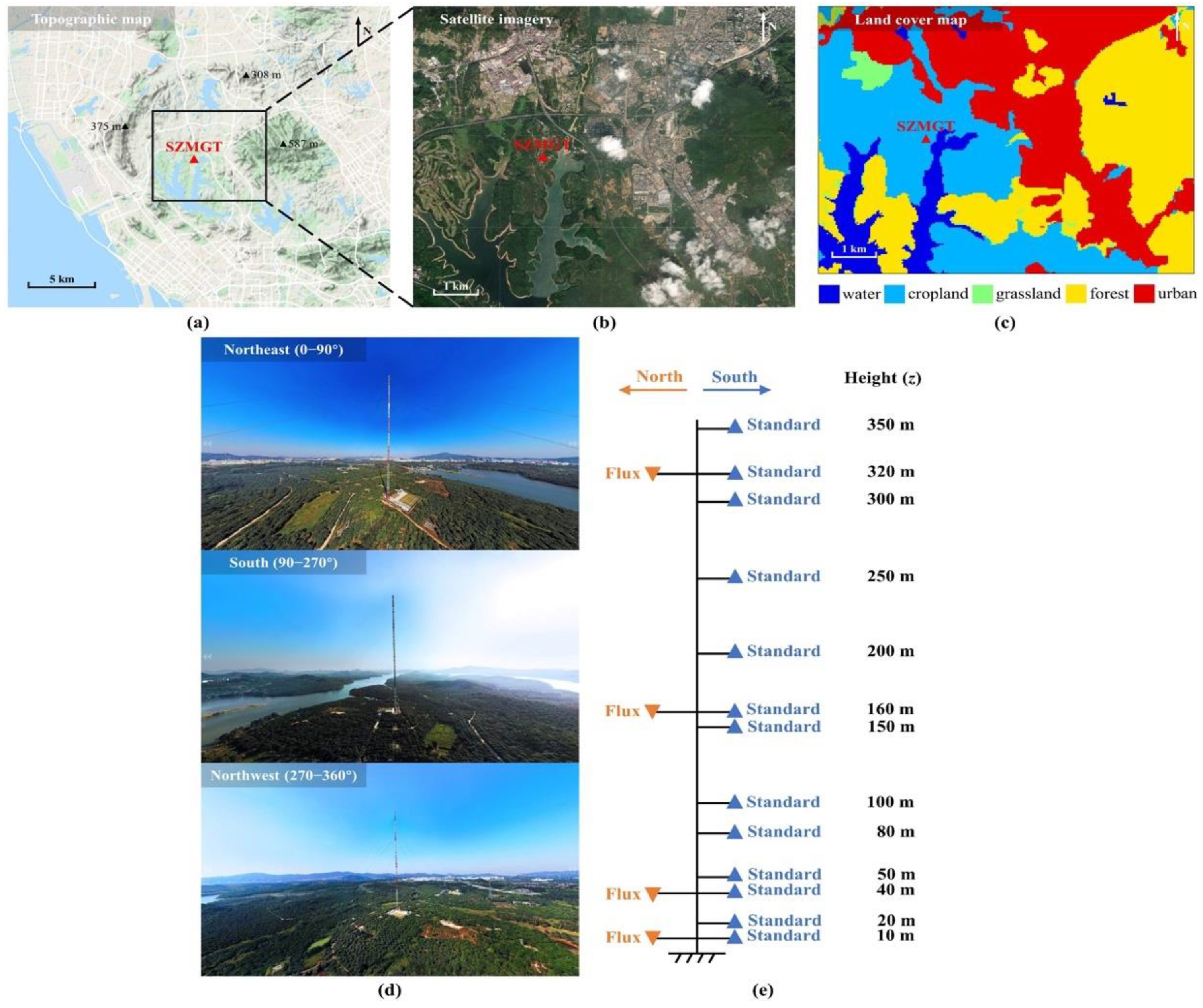
2.1. Site Description

The Shenzhen Meteorological Gradient Tower (SZMGT)at Tiegang Reservoir, Shenzhen, China (22°38′59″ N, 113°53′36″ E) is the source of the data in the present paper. The distance from the observation tower to the nearest shoreline was approximately 10 km and to the built-up area was about 1 km [30]. The SZMGT is an open lattice structure design with a total height of 365 m, and a cross-section of 2.5 m width [31,32,33]. This is the tallest observation tower in China, and the second tallest lattice observation tower worldwide. The terrain conditions around the SZMGT are illustrated in Figure 1, which generally features a suburban condition. To the north and east of SZMGT, the terrain is relatively flat, with 3-m-high broad-leaved evergreen plants, lakes and roads within a radius of 1 km, while the adjacent terrain in the south and west of SZMGT is quite uniform, with forests and lakes within a radius of 5 km as the main terrain [33].

2.2. Data Collection

Turbulence observations were made with four fast response 3D sonic anemometers (CSAT3, manufactured by Campbell Scientific) installed at 10 m, 40 m, 160 m and 320 m above the ground, respectively (see Table 1). These CSAT3 anemometers were pre-configured to measure three orthogonal wind components and virtual temperature at a sampling rate of 10 Hz. To minimize the airflow distortion caused by the physical structure of the meteorological tower, these sonic anemometers were installed on the beam 3.8 m north of the mast. Wind data included in this study were mainly recorded during several strong monsoon wind events, as shown in Table 2.

2.3. Data Quality Control

Prior to the characterization of the gustiness in tower-based wind observations, it is imperative to examine the quality of the data to gain a more accurate understanding of gust characteristics. As shown in Table 1, the CSAT3 sonic anemometers used in this study measured three orthogonal wind components (i.e., ux—along the west and east, pointing to the west positively; uy—along north and south, the positive direction points south, uz—vertical windward component); the sampling rate was 10 Hz. It should be noted that the original high-frequency observation data obtained by quick-response anemometer may sometimes be caused by various instrument problems or environmental factors (e.g., water contamination, rain drop, etc.) [34], leading to the occurrence of unexpected spikes in the time series. Hence, for each 10-min period in this study, five standard deviation filters were used to de-peak the three wind components [35]. All the spikes in the original time series were removed and refilled with an exponential filtering function [36]. The proportion of spikes in the raw high-frequency data was less than 5%.
After de-spiking, the three wind components perform further coordinate rotation every 10 min to generate 10 Hz estimates of longitudinal wind speed, u, transverse wind speed, v, and vertical wind speed, w, and average 10 for wind speed and horizontal direction [37]. The average ratio of the 3-s moving average of u, v, w to the total wind vector (i.e., u t , T 2 + v t , T 2 + w t , T 2 ) at the peak of gust is 0.98, 0.08 and 0.05. Therefore, all the studies of gust descriptors (as described in Section 3) were based on the 10-Hz time series of u [5], unless otherwise stated. In this study, a wind gust was defined as the maximum 3-s wind speed during each 10-min period.

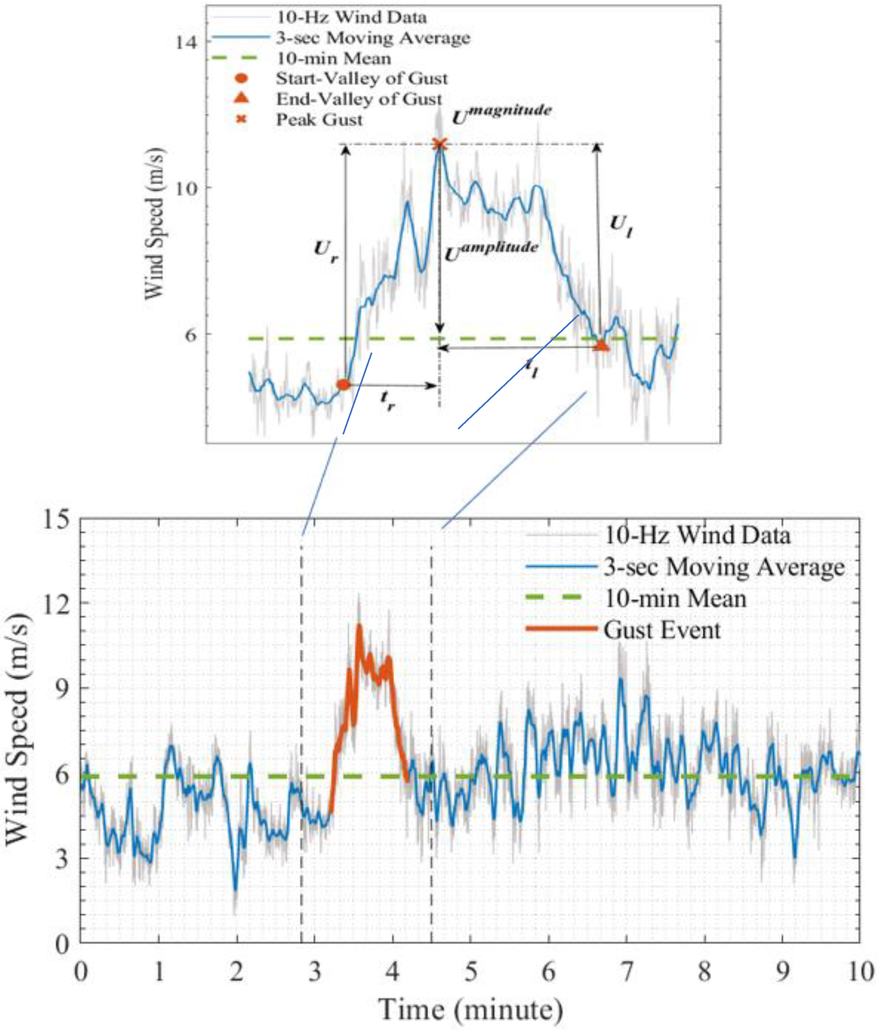
2.4. Definition of Wind Gust Descriptors

As mentioned above, the main objective of this study was to examine and discuss the gust characteristics through various gust descriptors. In light of the studies by Hu et al. [5], the major gust descriptors involved in the study are summarized as follows:
Gust peak magnitude u t , T m a x denotes the maximum 3 s moving average longitudinal wind speed u every 10-min period [8].
The amplitude of gust u t , T a represents the difference between the peak 3-s moving average gust speed and the 10-min average wind velocity U T (see Figure 2):
u t , T a = u t , T m a x U T
The gust coefficient G t , T is the ratio of the maximum value of peak gust u t , T m a x to the average wind speed in 10 min:
G t , T = u t , T m a x / U T
Likewise, the peak coefficient k t , T is the ratio of the gust amplitude u t , T a to the standard deviation σ T of the wind speed in 10 min:
k t , T = u t , T a / σ T
Turbulence intensity TI is the standard deviation of the 10 Hz longitudinal wind speeds, which is normalized by the 10 min average wind speed:
T I = σ T / U T
In addition to the aforementioned gust descriptors, the discrete gust events’ evolution in a time series can also be represented by four additional parameters, namely, the rise time t r , the lapse time t l , the rise magnitude u r , the lapse magnitude u l [5]. The rise time represents the time from the starting valley (i.e., the local minimum 3-s moving average immediately following below U T ) to the gust peak; the lapse time represents the time from the peak to trough (i.e., the next minimum value below U T in the moving average of 3-s). The increase was defined as the wind speed difference from the initial valley to the peak, whereas the drop was defined as the wind speed difference from the peak to the end valley (see Figure 2). Based on these four parameters, a gust asymmetrical factor (GAF) can be determined as:
G A F = u r / t r u l / t l
Moreover, the gust length scale L g is an estimate of the physical degree of a wind gust, which is described as the integral of the 3-s moving average of longitudinal wind speed throughout the gust:
L g = t s t a r t t e n d u 3 s d t
where t s t a r t and t e n d are the time of the start-valley and end-valley of the gust event, respectively. It is worth mentioning that the entire gust period is defined using the times of start-valley and end-valley, rather than the crossing times of U T and u 3 s , which ensures that the whole process of flow acceleration and deceleration is fully encapsulated [5].
For the classification of atmospheric stability, the Monin–Obukhov length [38] (L) is often used as a handy indicator, which can be calculated as follows:
L = u * 3 k ( g θ ) w θ ¯
where k is the von Karman constant (usually taken as 0.4), g is the gravitational acceleration (taken as 9.81 m/s2), θ is the virtual potential temperature, u * 3 is the cube of the friction velocity, w and θ represent the vertical wind velocity fluctuation component and the virtual potential temperature, respectively. In the present study, θ is approximated by sonic virtual temperature [39]; friction velocity u * can be determined as in [40].
u * = ( ( u w ¯ 2 + v w ¯ 2 ) 4
As shown in Table 3, the atmospheric stability condition of each 10-min wind speed segment is classified according to the classification scheme used by Barthelmie [41].

3. Results and Discussion

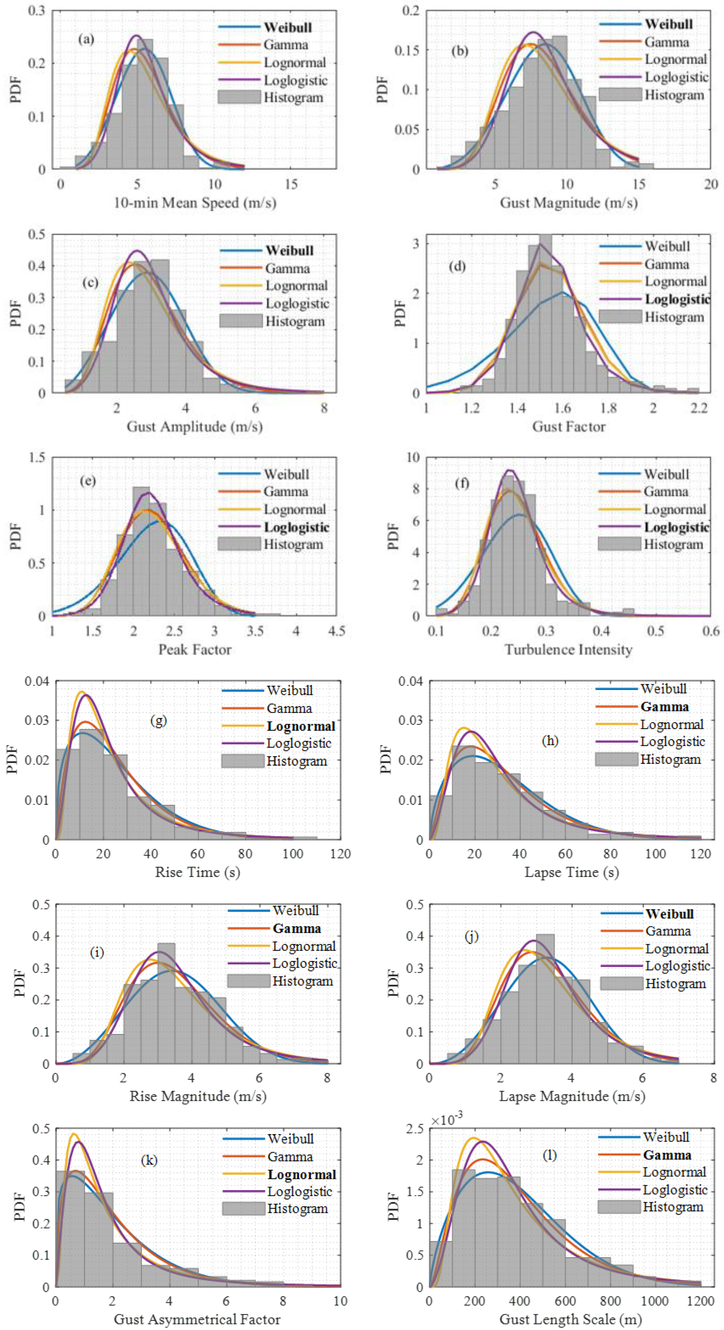
3.1. Distribution Fitting of Gust Description

It is to be noted that, although there exist many previous studies that have fitted various probability distributions to the average wind speed and gust amplitude, e.g., Weibull distribution [42,43,44,45] and Rayleigh distribution [46], few among them try to address which distribution form is most satisfactory. More importantly, the parent probability distribution that is closest to other gust characteristics distributions is seldom explored. Hence, four two-parameter distribution forms of positive-values (see Equations (9)–(12)) were employed in this study to fit the 12 gust descriptors by using maximum likelihood estimation (MLE). These distribution forms were selected mainly because all of the gust descriptive statistics were zero- bounded [5]. The data used herein were obtained at the observation level of 40 m high. The log-likelihood (LogL) value was adopted as an index to evaluate the performance of various distributions; the candidate distribution with the largest LogL value is considered to be the best fit [47]. Essentially, a likelihood method is a measure to describe how well a particular model fits the data. In statistics, the maximum likelihood estimation (MLE) is commonly used for estimating the parameters of an assumed probability distribution, given some observed data. When maximizing a likelihood function under the assumed statistical model, the observed data is most probable. Given that the logic of MLE is both intuitive and flexible, it has become a dominant means of statistical inference. Particularly, log-likelihood (LogL) is used mainly because it is computationally simpler and easier to optimize.
( 9 ) Weibull : f ( x | a , b ) = b a ( x a ) b 1 exp [ ( x a ) b ] ( 10 ) Gamma : f ( x | a , b ) = 1 b a Γ ( a ) x a 1 exp ( x b ) ( 11 ) Lognormal : f ( x | a , b ) = 1 x b 2 π exp [ ( ln ( x ) a ) 2 2 b ] ( 12 ) Log-logistic : f ( x | a , b ) = exp [ ln ( x ) a b ] b x { 1 + exp [ ln ( x a ) b ] } 2
Figure 3 and Table 4 summarize the distribution fitting of 12 gust descriptors considered in this study. The median gust magnitude and gust amplitude were, respectively, 8.49 m/s and 2.92 m/s. The results show that the Weibull distribution was the most suitable for the 10-min average wind speed, gust level and gust amplitude (Figure 3a–c), while the distribution of gust factor, peak factor and turbulence intensity (Figure 3d–f) could be most satisfactorily expressed as a logarithmic logic distribution. Although the Weibull distribution function is often used to fit the average wind speed and gust wind speed, Figure 3 clearly demonstrates that it is not appropriate for unitless parameters, such as gust factor, peak factor and turbulent intensity. The median values of rising time and elapsed time were estimated to be 19.8 s and 28.4 s, respectively; their distributions conformed most closely to the lognormal distribution and the gamma distribution, albeit with minor difference in the LogL values. As can be seen from Figure 3g,h, the distribution peak of rising time was more pronounced and skewed to the right than that of lapsing time. Hence, the consequent distribution of the gust asymmetric factor (Figure 3l) was also right-skewed, which can be most desirably described by the lognormal distribution. The median value of GAF was about 1.46. In the current study, the gust length scale ranged from 35.1 m to 1679.9 m, with a median value of 331.8 m. The distribution of the gust length scale was best fit by the gamma distribution, which is different from the conclusion by Hu et al. (2018), in which the log-normal distribution was shown to be the best-fitting for gust length scale. Moreover, the median rise and lapse magnitudes are 3.39 m/s and 3.25 m/s; their respective distributions follow the gamma distribution and Weibull distribution (Figure 3i,j) well.

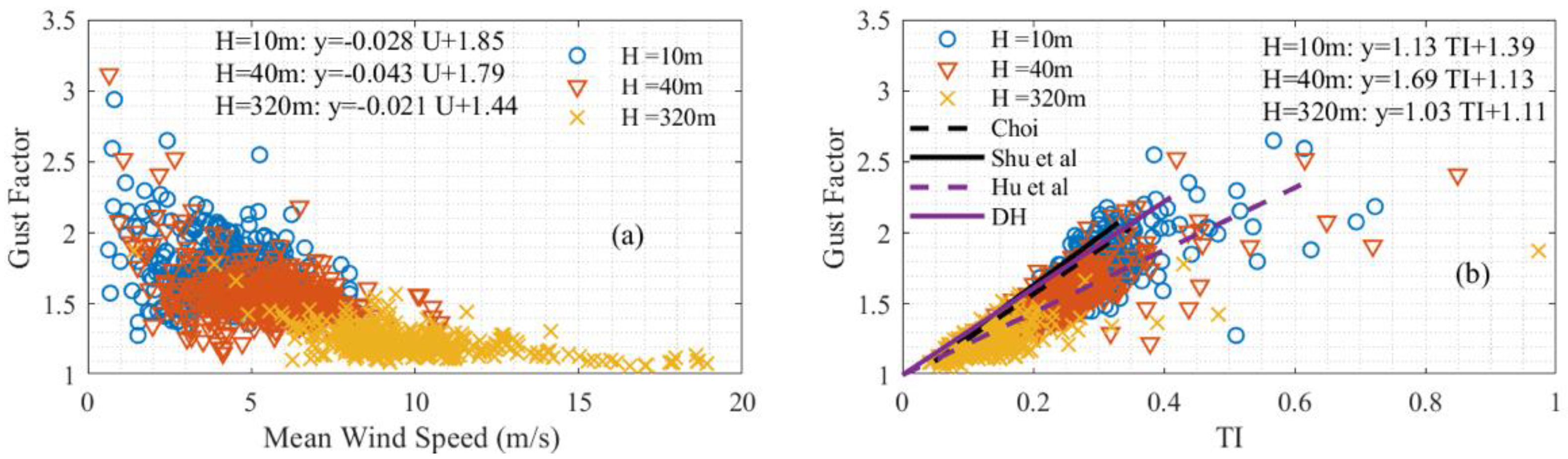
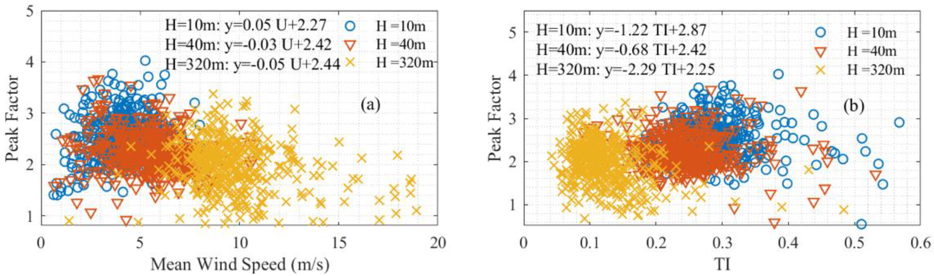
3.2. Gust Parameterizations

Besides the distribution fitting of gust descriptors, the parameterization of gusts is also of essential importance, particularly for numerical weather prediction (NWP) models, mainly because they do not explicitly address the gust [24]. A series of wind gust parameterization has been developed and applied to post-processing the output of the NWP model (e.g., [48]); conditional parameterizations based on observational data were also presented in many existing studies (e.g., [49]).
Figure 4 is the scatter diagram of the relationship between gust factor and 10-min average wind speed and turbulent intensity at three different heights (i.e., 10 m, 40 m and 320 m) based on observational data. In general, the gust factor values are negatively correlated with average wind speed; such a relationship may change slightly as a function of height. The slope coefficient of linear fits ranged from −0.043 to −0.021. Note that the dependence of gust factor on average wind speed derived in this study appears to be more pronounced than that obtained by Hu et al. [5], in which the fitted slope coefficient was about 0.0001. On the other hand, a strong positive correlation between the gust factor and the turbulence intensity can be seen in Figure 4. The slope coefficient from linear regression fits varied between 1.03 and 1.69; the intercept varied between about 1.11 and 1.39. In comparison with prior studies, the results showed that the results in this study indicate a good agreement with that presented by Hu et al. [5], whereas the regression fits by Choi [49], Deaves and Harris [50] tended to over-predict the gust factor.
Similarly, Figure 5 illustrates the respective relationship between peak factor and mean wind speed, as well as turbulent intensity. Hu et al. [5] reported that the peak factor failed to exhibit a significant linear dependence on either mean wind speed or turbulent intensity. As shown in Figure 5a, the dependence of peak factor on the average wind speed was, indeed, weak, with a slope coefficient ranging from −0.05 to 0.05. The subsequent intercept was between 2.27 and 2.44, which is close to the constant peak factor (~2.2) obtained by Bardal and Sætran [48]. Meanwhile, the peak factor obtained at different heights exhibited a consistent negative dependence on turbulent intensity. The slope coefficient was about −0.68 to −2.29; the intercepts ranged from 2.25 to 2.87.

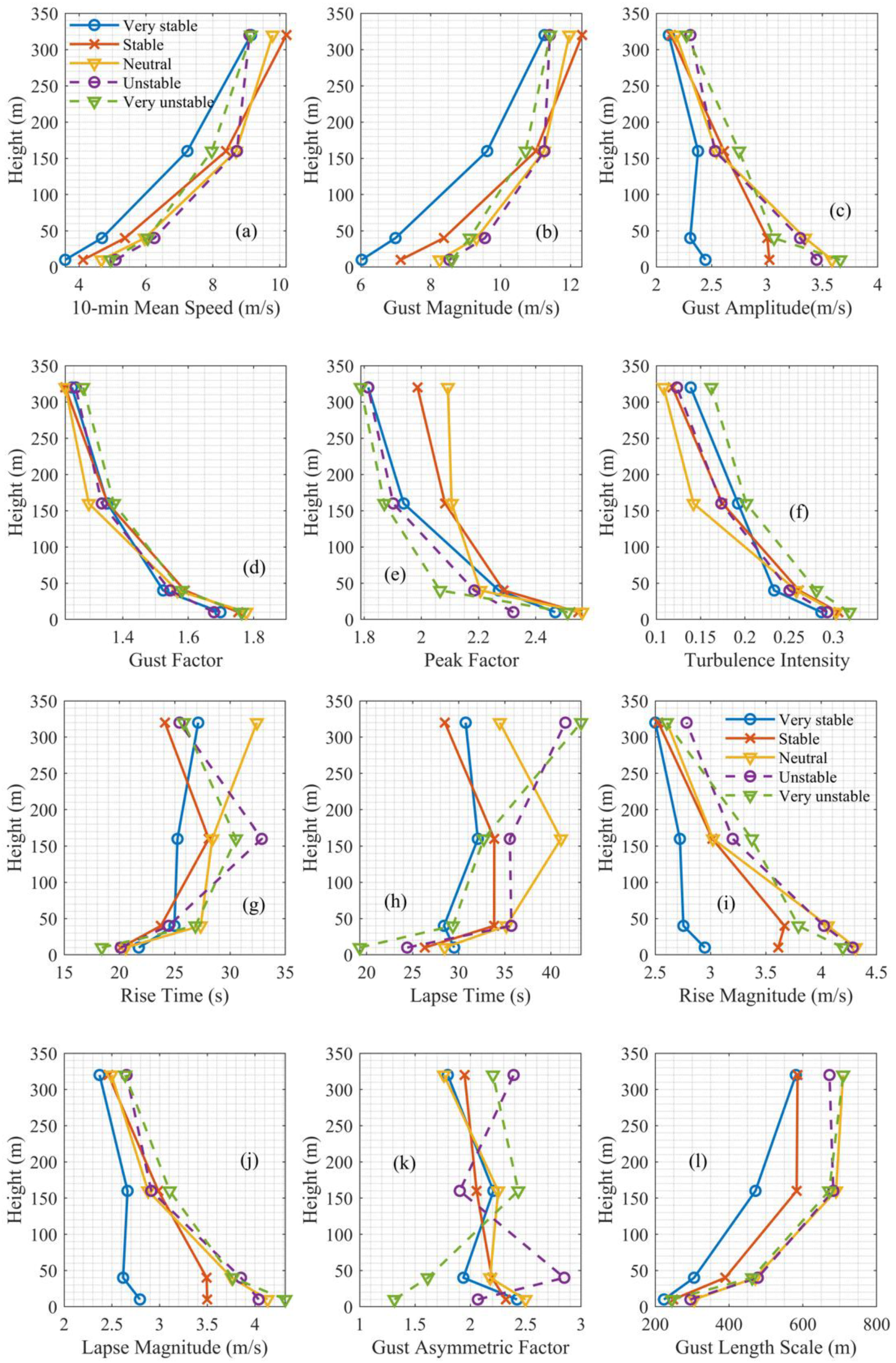
3.3. Vertical Profiles of Gust Descriptors

Furthermore, in order to examine the dependence of various gust descriptors on observation height, the entire data were conditionally grouped according to the estimated Monin–Obukhov length for each 10-min period; subsequently the data within each group were analysed in a composite sense. Figure 6 depicts the vertical extent of the median value of the gust descriptors, which appeared to reveal a certain degree of dissimilarity. For example, it was found that the 10-min average wind speed and gust amplitude increased monotonously with height. It should also be noted that the average wind speed and gust magnitude corresponding to very stable conditions tended to be somewhat smaller in magnitude than those in other atmospheric stability conditions, especially at lower levels.
The vertical profiles associated with gust amplitude, rise magnitude and lapse magnitude are more or less consistent, where the magnitude under very stable conditions remains relatively constant or decreases modestly as the observation height increase. By contrast, the profiles under the remaining atmospheric stability conditions exhibited a moderate downward trend with increasing height. For gust factor and turbulence intensity, the magnitudes generally decrease in parallel with the increase in height; the deviation of profiles corresponding to different stability conditions was found to be minor. The peak factor also decreases with increasing height, and the rate of such a decrease is closely tied with stability condition. It was clearly shown that the peak factor under stable and neutral conditions decreased more slowly than those in other conditions. On the other hand, the definition of vertical structure of rising time, elapsed time and gust asymmetry factor was less clear. As for the gust length scale, the vertical profile was similar to those of mean wind speed and gust magnitude, which typically indicates a positive dependence on height. Moreover, under very stable and stable conditions, the amplitude of the gust length scale is smaller than that under other stable conditions.

4. Concluding Remarks

Enhanced understanding of wind gust characteristics is critically important for a wide variety of practical applications. In the current study, a comprehensive assessment of the descriptors of wind gust was carried out based on high-resolution wind data from four heights of the meteorological tower. Conclusions are summarized as follows:
  • The probability distribution that most accurately represented the 12 wind gust descriptors was somewhat different. Specifically, the Weibull distribution was the most appropriate for those parameters, with length per time for units, such as 10-min average wind speed, gust magnitude, gust amplitude and elapsed amplitude. The unitless parameters, e.g., gust factor, peak factor and turbulence intensity, were best fitted by log-logistic distribution. The rising time and gust asymmetry factor exhibited lognormal distribution, while the Gamma distribution adequately described the distribution of gust length scale, rising amplitude and elapsed time.
  • The respective dependence of gust factor and peak factor on average wind speed and turbulent intensity was strongly tied with height. Note that gust factors were displayed as a linear function of turbulence intensity. Nevertheless, the empirical linear formulas given in previous studies have tended to over-predict.
  • The vertical extent of gust descriptors appeared to exhibit different profile shapes. In general, the 10-min average wind speed, gust amplitude and gust length scale are found to increase monotonically with height, whereas the gust amplitude, peak factor, gust factor, turbulence intensity, rising amplitude and elapsed amplitude tended to decrease as a function of height. For several gust descriptors, e.g., 10-min average wind speed and gust length scale, the magnitude of the vertical profile may vary with atmospheric stability condition.

Author Contributions

B.Y.: Writing- review and editing, Funding.; P.C.: Resources; Q.L.: Writing—review and editing; Y.H.: Resources, Writing—review and editing; Z.S.: Writing—original draft, Formal analysis, Methodology and investigation; Y.C. (Ying Cai): Funding, resources, writing—review and editing; Y.C. (Yao Chen): Writing—review and editing. All authors have read and agreed to the published version of the manuscript.

Funding

The work described in this paper was financially supported by grants from National Natural Science Foundation of China (Project Nos: 51878104), 111 Project of China (B18062), China Postdoctoral Science Foundation (2018M831063), Key Support Project for Overseas Expertise (zcsf2021008).

Data Availability Statement

The datasets analysed during the current study are available from the corresponding author on reasonable request.

Acknowledgments

The authors would like to thank Hong Kong Observatory and Meteorological Bureau of Shenzhen Municipality for sharing the data analysed in this paper.

Conflicts of Interest

The authors declare no competing interest.

References

  1. Yan, B.; Chan, P.; Li, Q.; He, Y.; Shu, Z. Characterising the fractal dimension of wind speed time series under different terrain conditions. J. Wind Eng. Ind. Aerodyn. 2020, 201, 104165. [Google Scholar] [CrossRef]
  2. Boettcher, F.; Renner, C.; Waldl, H.-P.; Peinke, J. On the statistics of wind gusts. Boundary-Layer Meteorol. 2003, 108, 163–173. [Google Scholar] [CrossRef]
  3. Shu, Z.R.; Chan, P.W.; Li, Q.S.; He, Y.C.; Yan, B.W. Quantitative assessment of offshore wind speed variability using fractal analysis. Wind. Struct. 2020, 31, 363–371. [Google Scholar]
  4. He, Y.; He, J.; Chen, W.; Chan, P.; Fu, J.; Li, Q. nsights from Super Typhoon Mangkhut (1822) for wind engineering practices. J. Wind Eng. Ind. Aerodyn. 2020, 203, 104238. [Google Scholar] [CrossRef]
  5. Hu, W.; Letson, F.; Barthelmie, R.J.; Pryor, S.C. Wind gust characterization at wind turbine relevant heights in moderately complex terrain. J. Appl. Meteorol. Clim. 2018, 57, 1459–1476. [Google Scholar] [CrossRef]
  6. Gutiérrez, A.; Porrini, C.; Fovell, R.G. Combination of wind gust models in convective events. J. Wind Eng. Ind. Aerodyn. 2020, 199, 104118. [Google Scholar] [CrossRef]
  7. Suomi, I.; Gryning, S.; Floors, R.; Vihma, T.; Fortelius, C. On the vertical structure of wind gusts. Q. J. R. Meteorol. Soc. 2015, 141, 1658–1670. [Google Scholar] [CrossRef]
  8. WMO. Measurement of surface wind. In Guide to Meteorological Instruments and Methods of Observation; WMO-No. 8; 2008 Edition Updated in 2010; World Meteorological Organization: Geneva, Switzerland, 2012. [Google Scholar]
  9. Letson, F.; Barthelmie, R.J.; Hu, W.; Brown, L.D.; Pryor, S.C. Wind gust quantification using seismic measurements. Nat. Hazards 2019, 99, 355–377. [Google Scholar] [CrossRef]
  10. Friederichs, P.; Göber, M.; Bentzien, S.; Lenz, A.; Krampitz, R. A probabilistic analysis of wind gusts using extreme value statistics. Meteorol. Z. 2009, 18, 615–629. [Google Scholar] [CrossRef]
  11. Pasztor, F.; Matulla, C.; Zuvela-Aloise, M.; Rammer, W.; Lexer, M.J. Developing predictive models of wind damage in Austrian forests. Ann. For. Sci. 2015, 72, 289–301. [Google Scholar] [CrossRef] [Green Version]
  12. Suomi, I.; Gryning, S.; O’Connor, E.J.; Vihma, T. Methodology for obtaining wind gusts using Doppler lidar. Q. J. R. Meteorol. Soc. 2017, 143, 2061–2072. [Google Scholar] [CrossRef] [Green Version]
  13. Jung, C.; Schindler, D.; Albrecht, A.T.; Buchholz, A. The role of highly-resolved gust speed in simulations of storm damage in forests at the landscape scale: A case study from southwest Germany. Atmosphere 2016, 7, 7. [Google Scholar] [CrossRef] [Green Version]
  14. Brasseur, O. Development and application of a physical approach to estimating wind gusts. Mon. Weather Rev. 2001, 129, 5–25. [Google Scholar] [CrossRef]
  15. Fang, G.; Zhao, L.; Cao, S.; Ge, Y.; Li, K. Gust characteristics of near-ground typhoon winds. J. Wind Eng. Ind. Aerodyn. 2019, 188, 323–337. [Google Scholar] [CrossRef]
  16. Suomi, I.; Vihma, T. Wind gust measurement techniques—From traditional anemometry to new possibilities. Sensors 2018, 18, 1300. [Google Scholar] [CrossRef] [Green Version]
  17. Ágústsson, H.; Ólafsson, H. Forecasting wind gusts in complex terrain. Arch. Meteorol. Geophys. Bioclimatol. Ser. B 2009, 103, 173–185. [Google Scholar] [CrossRef]
  18. Hewston, R.; Dorling, S.R. An analysis of observed daily maximum wind gusts in the UK. J. Wind Eng. Ind. Aerodyn. 2011, 99, 845–856. [Google Scholar] [CrossRef] [Green Version]
  19. Shu, Z.; Li, Q.; He, Y.; Chan, P.W. Gust factors for tropical cyclone, monsoon and thunderstorm winds. J. Wind Eng. Ind. Aerodyn. 2015, 142, 1–14. [Google Scholar] [CrossRef]
  20. He, J.; Li, Q.; Chan, P. Reduced gust factor for extreme tropical cyclone winds over ocean. J. Wind Eng. Ind. Aerodyn. 2021, 208, 104445. [Google Scholar] [CrossRef]
  21. Türk, M.; Emeis, S. The dependence of offshore turbulence intensity on wind speed. J. Wind Eng. Ind. Aerodyn. 2010, 98, 466–471. [Google Scholar] [CrossRef]
  22. Letson, F.; Barthelmie, R.J.; Hu, W.; Pryor, S.C. Characterizing wind gusts in complex terrain. Atmospheric Chem. Phys. 2019, 19, 3797–3819. [Google Scholar] [CrossRef] [Green Version]
  23. Burton, T.; Sharpe, D.; Jenkins, N.; Bossanyi, E. Wind Energy Handbook; Wiley: New York, NY, USA, 2001; Volume 2. [Google Scholar]
  24. Suomi, I.; Vihma, T.; Gryning, S.-E.; Fortelius, C. Wind-gust parametrizations at heights relevant for wind energy: A study based on mast observations. Q. J. R. Meteorol. Soc. 2013, 139, 1298–1310. [Google Scholar] [CrossRef]
  25. Beljaars, A.C.M. The influence of sampling and filtering on measured wind gusts. J. Atmospheric Ocean. Technol. 1987, 4, 613–626. [Google Scholar] [CrossRef] [Green Version]
  26. Greenway, M. An analytical approach to wind velocity gust factors. J. Wind Eng. Ind. Aerodyn. 1979, 5, 61–91. [Google Scholar] [CrossRef]
  27. International Electrotechnical Commission. Wind Turbines-Part 1: Design Requirements; IEC 614001 Ed. 3; International Electrotechnical Commission: Geneva, Switzerland, 2006. [Google Scholar]
  28. Manwell, J.F.; McCowan, J.G.; Rogers, A.L. Bind Energy Explained: Theory, Design and Application; John Wiley & Sons: Hoboken, NJ, USA, 2010. [Google Scholar]
  29. Bierbooms, W.; Cheng, P.-W. Stochastic gust model for design calculations of wind turbines. J. Wind Eng. Ind. Aerodyn. 2002, 90, 1237–1251. [Google Scholar] [CrossRef]
  30. Li, L.; Lu, C.; Chan, P.-W.; Zhang, X.; Yang, H.-L.; Lan, Z.-J.; Zhang, W.-H.; Liu, Y.-W.; Pan, L.; Zhang, L. Tower observed vertical distribution of PM2. 5, O3 and NOx in the Pearl River Delta. Atmospheric Environ. 2020, 220, 117083. [Google Scholar] [CrossRef]
  31. Luo, Y.P.; Fu, J.Y.; Li, Q.S.; Chan, P.W.; He, Y.C. Observation of Typhoon Hato based on the 356-m high meteorological gradient tower at Shenzhen. J. Wind. Eng. Ind. Aerodyn. 2020, 207, 104408. [Google Scholar] [CrossRef]
  32. He, J.; He, Y.; Li, Q.; Chan, P.; Zhang, L.; Yang, H.; Li, L. Observational study of wind characteristics, wind speed and turbulence profiles during Super Typhoon Mangkhut. J. Wind Eng. Ind. Aerodyn. 2020, 206, 104362. [Google Scholar] [CrossRef]
  33. He, J.; Chan, P.; Li, Q.; Li, L.; Lu, C.; Zhang, L.; Yang, H. Characteristics of Wind Structure and Nowcasting of Gust Associated with Subtropical Squall Lines over Hong Kong and Shenzhen, China. Atmosphere 2020, 11, 270. [Google Scholar] [CrossRef] [Green Version]
  34. Aubinet, M.; Vesala, T.; Papale, D. (Eds.) Eddy Covariance: A Practical Guide to Measurement and Data Analysis; Springer Science & Business Media: Berlin/Heidelberg, Germany, 2012. [Google Scholar]
  35. Masters, F.J.; Vickery, P.J.; Bacon, P.; Rappaport, E.N. Toward objective, standardized intensity estimates from surface wind speed observations. Bull. Am. Meteorol. Soc. 2010, 91, 1665–1682. [Google Scholar] [CrossRef]
  36. Hojstrup, J. A statistical data screening procedure. Meas. Sci. Technol. 1993, 4, 153–157. [Google Scholar] [CrossRef]
  37. Foken, T.; Napo, C.J. Micrometeorology; Springer: Berlin/Heidelberg, Germany, 2008; Volume 2. [Google Scholar]
  38. Monin, A.S.; Obukhov, A.M. Basic laws of turbulent mixing in the surface layer of the atmosphere. Contrib. Geophys. Inst. Acad. Sci. USSR 1954, 151, e187. [Google Scholar]
  39. Kaimal, J.C.; Gaynor, J.E. Another look at sonic thermometry. Boundary-Layer Meteorol. 1991, 56, 401–410. [Google Scholar] [CrossRef]
  40. Weber, R.O. Remarks on the definition and estimation of friction velocity. Boundary-Layer Meteorol. 1999, 93, 197–209. [Google Scholar] [CrossRef]
  41. Barthelmie, R.J. The effects of atmospheric stability on coastal wind climates. Meteorol. Appl. 1999, 6, 39–47. [Google Scholar] [CrossRef]
  42. Dimitrov, N. Comparative analysis of methods for modelling the short-term probability distribution of extreme wind turbine loads. Wind Energy 2016, 19, 717–737. [Google Scholar] [CrossRef]
  43. Shu, Z.; Li, Q.; Chan, P.W. Statistical analysis of wind characteristics and wind energy potential in Hong Kong. Energy Convers. Manag. 2015, 101, 644–657. [Google Scholar] [CrossRef]
  44. Shu, Z.; Li, Q.; Chan, P.W. Investigation of offshore wind energy potential in Hong Kong based on Weibull distribution function. Appl. Energy 2015, 156, 362–373. [Google Scholar] [CrossRef]
  45. Shu, Z.R.; Li, Q.S.; He, Y.C.; Chan, P.W. Observations of offshore wind characteristics by Doppler-LiDAR for wind energy applications. Appl. Energy 2016, 169, 150–163. [Google Scholar] [CrossRef]
  46. Cheng, P.; Bierbooms, W. Distribution of extreme gust loads of wind turbines. J. Wind Eng. Ind. Aerodyn. 2001, 89, 309–324. [Google Scholar] [CrossRef]
  47. Hogg, R.V.; McKean, J.; Craig, A.T. Introduction to Mathematical Statistics; Pearson Education: New York, NY, USA, 2005. [Google Scholar]
  48. Bardal, L.M.; Sætran, L.R. Wind gust factors in a coastal wind climate. Energy Procedia 2016, 94, 417–424. [Google Scholar] [CrossRef] [Green Version]
  49. Choi, C.C. Wind Loading in Hong Kong: Commentary on the Code of Practice on Wind Effects Hong Kong; Hong Kong Institution of Engineers: Hong Kong, 1983. [Google Scholar]
  50. Deaves, D.M.; Harris, R.I. A Mathematical Model of the Structure of Strong Winds; CIRIA Report 76; Construction Industry Research and Information Association: London, UK, 1978. [Google Scholar]
Figure 1. The meteorological gradient tower used in the current study. (a) topographic map, (b) satellite map, (c) land cover map, (d) photos of terrain exposures, (e) installation heights of measurement devices.
Applsci 12 02105 g001
Figure 2. A diagram of a single gust event showing the gust descriptors.
Applsci 12 02105 g002
Figure 3. Probability density histogram and distribution fitting of observed data. The four types of two-parameter positive-valued distribution used in distribution fitting are Weibull, Gamma, Lognormal and Log-logistic. For each gust parameter, the optimal distribution (bolded) was identified according to the maximum Log-likelihood (LogL), as shown in Table 4. (a) 10-min average wind speed, (b) gust amplitude, (c) gust amplitude, (d) gust coefficient, (e) peak coefficient, (f) turbulent intensity, (g) rising time, (h) elapsed time, (i) rising amplitude, (j) elapsed amplitude, (k) gust asymmetry coefficient and (l) gust length scale.
Applsci 12 02105 g003
Figure 4. Scatter diagram: (a) gust factor vs. 10-min average wind speed; (b) gust factor vs. turbulence intensity. In (b), the empirical results from Shu et al. (2015), Choi (1984), Hu et al. (2018) and Deaves and Harris (1978) are also depicted for comparison.
Applsci 12 02105 g004
Figure 5. Scatter diagram: (a) peak factor vs. 10-min average wind speed; (b) peak factor vs. turbulence intensity.
Applsci 12 02105 g005
Figure 6. Vertical profiles of gust descriptors as a function of atmospheric stability condition. (a) 10-min average wind speed, (b) gust amplitude, (c) gust amplitude, (d) gust coefficient, (e) peak coefficient, (f) turbulent intensity, (g) rising time, (h) elapsed time, (i) rising amplitude, (j) elapsed amplitude, (k) gust asymmetry amplitude and (l) gust length scale.
Applsci 12 02105 g006
Table 1. Information of the observation data.
InstrumentHeight (m)Observation ElementOutput Frequency
3D (Three dimensional) sonic anemometer (CSAT3)10, 40, 160, 320 above the level of groundThree orthogonal wind components (ux, uy, uz), sonic virtual temperature (Ts)10 Hz
Table 2. Outline of the observation period involved in the current study.
YearStartEnd
201815 September 00:0017 September 23:59
20188 January 20:008 January 23:59
20189 January 00:009 January 11:00
20188 March 00:008 March 11:00
20187 April 00:007 April 09:00
20194 March 20:004 March 23:59
20195 March 00:005 March 04:00
201922 September 06:0022 September 11:00
20197 October 00:007 October 08:00
202016 February 00:0016 February 17:00
Table 3. Classification of atmospheric stability condition [41].
Stability ClassRange of Monin–Obukhov Length (m)
Unstable (u) 1000 < L < 200
Very unstable (vu) 200 < L < 0
Very stable (vs) 0 < L < 200
Stable (s) 200 < L < 1000
Neutral (n) | L | > 1000
Table 4. Summary of log-likelihood (LogL) estimation.
Mean SpeedGust AmplitudeGust AmplitudeGust FactorPeak FactorTI
Weibull−846.3−1008.7−612.2128.8−199.8615.9
Gamma−870.1−1028.5−617.6202.4−174.8641.9
Log-Normal−901.2−1050.6−637.2206.7−176.7632.4
Log-Logistic−875.2−1037.9−626.0215.2−174.4659.5
Rise TimeLapse TimeRise MagnitudeLapse MagnitudeGAFLg
Weibull−1752.3−1905.1−733.3−689.9−767.8−2930.8
Gamma−1743.8−1896.7−730.3−690.4−761.7−2927.8
Log-Normal−1739.7−1899.7−744.8−707.6−742.7−2940.6
Log-Logistic−1752.4−1905.6−738.3−697.7−749.0−2944.7
Publisher’s Note: MDPI stays neutral with regard to jurisdictional claims in published maps and institutional affiliations.

