Article

An Elliptic Blending Turbulence Model-Based Scale-Adaptive Simulation Model Applied to Fluid Flows Separated from Curved Surfaces

1
College of Civil and Transportation Engineering, Shenzhen University, Shenzhen 518060, China
2
Key Laboratory for Resilient Infrastructures of Coastal Cities (MOE), Shenzhen University, Shenzhen 518060, China
*
Author to whom correspondence should be addressed.
Appl. Sci. 2022, 12(4), 2058; https://doi.org/10.3390/app12042058
Submission received: 24 December 2021 / Revised: 7 February 2022 / Accepted: 11 February 2022 / Published: 16 February 2022

Abstract

:
On the basis of a previously developed elliptic blending turbulence model (SST–kωφα model), a scale-adaptive simulation (SAS) model is developed by following Menter and Egorov’s SAS concept. An SAS source term, which is related to the ratio of the modeled turbulence scale to the von Kármán length scale, is introduced into the corresponding length-scale determining equation. The major motivation of this study is that the conventional unsteady Reynolds-averaged Navier–Stokes (URANS) models provide only large-scale unsteadiness. The introduction of the SAS term allows the proposed SAS model to dynamically adjust to resolved structures in a URANS framework because this term is sensitive to resolved fluctuations. The predictive capabilities of the proposed SAS model are demonstrated by computing the complex flow configurations in three cases with flow separation from curved surfaces, namely, three-dimensional (3D) diffuser flow, two-dimensional (2D) periodic hills flow, and 2D U-turn duct flow. For comparison, the results predicted by the SST–kωφα model and the Menter and Egorov’s SAS model (SST–SAS) are provided. The results are also compared with the relevant experimental, direct numerical simulation, and large eddy simulation data. The results show that the SST–kωφα model cannot capture the critical features for all three flows, and that the SST–SAS model is able to predict the results reasonably well. The proposed SAS model is capable of resolving more portions of the turbulence structures, and it yields the best results in all the cases.

1. Introduction

Turbulence is a three-dimensional (3D), time-dependent, nonlinear, and ubiquitous phenomenon in nature. Fully understanding turbulence is a goal that people have been pursuing for several years. With the advent and continuous development of computers, the use of numerical simulation methods to study turbulence has also made great progress. Numerical simulation of turbulence is a very important issue, especially in engineering fields. It can help people save a considerable amount of money and shorten design time by avoiding the need to build and test prototypes.
To date, owing to limitations in computing power, direct numerical simulation (DNS) of turbulence is still difficult to achieve in engineering problems [1]. A practical method is to model turbulence. There are two typical methods for modeling turbulence: Reynolds-averaged Navier–Stokes (RANS) and large eddy simulation (LES). For many years, RANS models have offered the most economic approach and have been widely used in industrial applications. In RANS models, all turbulent structures are eliminated from the flow. This treatment greatly reduces the accuracy. LES is based on the approach of resolving large turbulent structures in space down to the grid limit everywhere in the flow. With LES, most of the turbulence spectra are resolved, and better results can usually be obtained. However, owing to the excessively high-resolution requirements for wall boundary layers, LES has a very limited impact on industrial simulation. Hybrid RANS–LES approaches have become increasingly popular in recent years as methods that maintain a balance between accuracy and cost [2]. Hybrid RANS–LES approaches incorporate the advantages of the RANS and LES models. Specifically, the attached wall boundary layers are covered by the RANS model; thus, the excessive resolution requirements of LES can be avoided. Meanwhile, the large, detached regions are handled in the LES mode, i.e., with a partial resolution of the turbulent spectrum.
Hybrid RANS–LES approaches have been developed by many researchers. Owing to space limitations, they are not reviewed comprehensively here. Interested readers can refer to the reviews in [3,4]. However, it is worth briefly reviewing one of them, the scale-adaptive simulation (SAS), which is utilized in this study. By revisiting the kL model of Rotta, the SAS model was developed by Menter and Egorov [5]. An additional source term consisting of the von Kármán length scale is introduced into the scale-determining equation of the relevant unsteady RANS (URANS) model. When the flow is strongly unstable, this term can reduce the computed length scale, thus yielding a lower eddy viscosity, which in turn allows flow fluctuations to be sustained. The SAS method has several advantages, a few of which are described. First, it is very easy to implement it into an existing URANS model (simply by inserting an additional source term into the scale-determining equation). Second, it does not contain any parameters related to grid size. It is generally known that when the grid resolution is not sufficiently fine, the models related to grid size yield poor results (for instance, the detached eddy simulation (DES) [5] and LES [6] models). Nevertheless, if the grid resolution is not sufficiently fine, the SAS model provides the URANS performance, which is reasonably capable of handling the flow. This feature seems attractive and can be regarded as a safeguard in the simulation of complex industrial flows [3].
Obviously, the performance of the SAS model depends on the RANS model used. The SAS model was originally developed based on the k k L model, and was then transformed into the kε model, the kω model, and the well-known shear stress transport (SST) kω model [5]. The most widely used SAS model is based on the SST kω model. Among the many RANS models, there is a class of models that are very attractive, namely, the elliptic blending or elliptic relaxation-based models. The basis of this type of model is the v 2 ¯ f model developed by Durbin [7]. Since then, many variants have evolved. These models can be divided into three categories: one stems from the kε model, the second stems from the Reynolds stress model, and the third stems from the kω model. Research on the first two categories began earlier, and many results have been obtained. For detailed reviews of these models, readers can refer to Billard and Laurence [8] and Manceau [9]. Research on the kω-based models started relatively late, and the early developments of these models were reviewed by Yang et al. [10,11]. Recently, Biswas et al. [12] developed an elliptic blending lag model based on the conventional kω model. Shang and Agarwal [13] developed an elliptic blending lag model based on the conventional SST kω model. The present authors [14] developed an elliptic blending turbulence model by transforming the kε-based BL v 2 ¯ / k model of Billard and Laurence [8] into a kω system. Additionally, the SST characteristics in the boundary layer were integrated, and the model performance was greatly improved. Generally, kω-based models have better stability than others [10,11].
There are very few SAS models based on elliptic blending or elliptic relaxation models. The only one found in the literature was developed by Krumbein et al. [15]. They proposed an SAS model based on the elliptic relaxation model of Hanjalić et al. [16] (the ζf model). The model was validated by computing several generic flow configurations with relatively coarse meshes, including the channel flow, flow over periodic hills, flow over fence, impinging jet, and flow mixing in the T-junction. The results are encouraging.
In this study, an SAS model, which is based on an elliptic blending model (denoted as the SST–kωφα model) previously developed by the authors [14], was proposed and validated. In the next section, the formulation of the model and its implementation are briefly described. In the third section, the performance of the model is investigated by applying it to three flow configurations: 3D asymmetric diffuser flow, flow over two-dimensional (2D) periodic hills, and 2D U-turn duct flow. Lastly, the conclusions are presented.

2. Model Formulation and Implementation

The basis of the proposed SAS model is the SST–kωφα model, which belongs to the elliptic blending RANS model category [14]. The SAS model consists of four model equations for the turbulent kinetic energy k, specific dissipation rate ω, wall-normal turbulent anisotropy φ, and elliptic variable α. The equations of the model are as follows:
ρ k t + x i ( ρ u i k ) = G k ρ f k β k ω + x j [ ( μ 2 + σ k μ t ) k x j ] ,
ρ ω t + x i ( ρ u i ω ) = f ω γ ω k G k ρ β ω 2 + C D + x j [ ( μ 2 + σ ω μ t ) ω x j ] + Q S A S ,
ρ ϕ t + x i ( ρ u i ϕ ) = ( 1 α p ) ρ f wall + α p ρ f hom ϕ k G k + 2 k μ t σ k ϕ x j k x j + x j [ ( μ 2 + σ ϕ μ t ) ϕ x j ] ,
0 = 1 α L 2 + x j ( α x j ) .
In addition, an additional source term QSAS is introduced into the ω-equation, and the remaining terms are the same as the SST–kωφα model. For the meaning of each term and the value of each coefficient, please refer to Yang et al. [14].
The source term QSAS is the same as the SST kω model-based SAS model (denoted as the SST–SAS model) [5]. It is defined as follows:
Q S A S = max [ ρ η 2 κ S 2 ( L t L v k ) 2 C S A S 2 ρ k σ q max ( 1 k 2 k x j k x j , 1 ω 2 ω x j ω x j ) , 0 ] ,
with η 2 = 3.51 , κ = 0.41 , C S A S = 2 , and σ q = 2 / 3 . The modeled turbulence length scale and the von Kármán length scale are
L t = k c μ 2 ω ,
and
L v k = κ | U U | ,
respectively. Here, cμ = 0.09, U = S is the magnitude of the shear stress, and U is the magnitude of the velocity Laplacian, which is given by
U = 2 U i x j 2 2 U i x k 2 .
For the purpose of comparison, all test cases were computed using three models: the proposed SAS model (denoted as the SST–kωφα–SAS model), SST–SAS model, and SST–kωφα model. The FLUENT computational fluid dynamics (CFD) code was used as the computing platform. The SST–SAS model is built into the software itself. The proposed SAS and SST–kωφα models were implemented using the user-defined function (UDF) functionality.
A pressure-based coupled algorithm was used to solve the governing equation system. The bounded second-order implicit scheme was used for the integration of the transient terms. The bounded central differencing scheme and the second-order upwind scheme were used to discretize the convection terms in the momentum equation and in the turbulence equations, respectively. The gradients and derivatives were evaluated by the least-squares cell-based method.
In all cases, the successive ratio mesh was used in the vertical direction of the wall, and the first grid point adjacent to the wall was carefully placed to ensure that the condition of nondimensional wall distance y+ < 1 was satisfied. The no-slip condition was applied to the solid walls. However, in different models, the wall treatments were different. Specifically, for the SST–kωφα–SAS and SST–kωφα models, ui = 0, k = 0, φ = 0, α = 0, and ω w = 3 ν / ( β 0 y 1 2 ) [14]. For the SST–SAS model, an automatic near-wall treatment method was used [17]. At the outlets, a zero-gradient condition was applied for each variable except pressure. For the periodic boundary conditions occurring in this study, the pressure drop across the periodic planes was set to zero. At inlets, the values of the variables were problem-dependent and are stated later in the paper for each case. Additionally, the vortex method [18] was applied to generate random fluctuations at the inlets.

3. Results and Discussion

The performance of the proposed SAS model was illustrated by computing the complex flow configurations in three cases with boundary layer separation from curved surfaces, namely, the 3D asymmetric diffuser flow, 2D periodic hills flow, and 2D U-turn duct flow. The motivation for choosing these cases is that they present challenges to conventional RANS models. The SST–SAS and SST–kωφα models were adopted for comparison. In general, many factors may influence the results. For a reasonable comparison, for each case, all of the calculation conditions, such as the computational mesh, timestep size, discretization scheme, and Courant–Friedrichs–Lewy (CFL) number, were set the same or as close as possible for all three turbulence models.

3.1. 3D Asymmetric Diffuser Flow

To provide detailed and reliable data for the CFD model validation, Cherry et al. [19,20] designed a fully 3D diffuser flow and measured the velocity field and pressure distribution in detail. Using the same geometry and boundary conditions, a DNS was performed by Ohlsson et al. [21]. The DNS results were in good agreement with the measurements.
This case has been chosen to validate turbulence models by many researchers. For example, Billard et al. [22] considered the performances of four RANS turbulence models (the SST kω model of Menter [23], the BL v 2 ¯ / k model of Billard and Laurence [8], the Speziale–Sarkar–Gatski (SSG) model of Speziale et al. [24], and the elliptic blending Reynolds stress model (EBRSM) of Manceau and Hanjalić [25]) in this flow. It was found that only the EBRSM could predict reasonable results. Abe and Ohtsuka [26] simulated this case using a pure RANS model, a pure LES model, and a hybrid RANS–LES model. The same mesh with a moderate grid resolution was used for the three models. It was shown that the hybrid RANS–LES model yielded better results than the other models. The pure LES model failed because the grid resolution was insufficient. Jakirlic and Maduta [27] simulated the 3D diffuser flow using a RANS model and an SAS model. It was found that the results predicted by the SAS model were in good agreement with the experimental and DNS findings, but the results predicted by the RANS model were not.
Figure 1 showed a schematic of the geometry and relevant boundary conditions of the 3D diffuser flow used in this study. Consistent with the experiment [19] and DNS [21], the Reynolds number (Re) based on the bulk velocity at the inlet (Ub) and the height of the inlet duct (H) was 10,000. The fully developed profiles, which were extracted from a precursor simulation in a long duct at the same Re and with relevant turbulence models, were used at the inlet. The number of computational meshes was 3.24 million, which was similar to that used by Jakirlic and Maduta [27]. The timestep size was 0.02 H/Ub. The statistics began at 5000 steps and continued to 10,000 steps to ensure that the mean values of the variables remained unchanged with time.
The DNS data of Ohlsson et al. [21] were used as references. A comparison of the contours of the mean stream-wise velocity u ¯ at different cross-sections, which was normalized by Ub, is shown in Figure 2. At x/H = 2, both the SST–kωφα–SAS and the SST–SAS models predicted the flow separation at the top-right corner, where the two expanding walls intersect. However, the SST–SAS model incorrectly predicted a large separation at the top-left corner. The SST–kωφα model also predicted the flow separation at the top-right corner, but the separation bubble was too large compared to that predicted by the DNS. Compared with the DNS, both the SST–kωφα–SAS and the SST–SAS models predicted an earlier separation near the top-left corner (see the contours at x/H = 5), but a delayed separation near the center of the top wall (see the contours at x/H = 8). The proposed SAS model was better than the SST–SAS model in terms of predicting the location of the maximum velocity. At x/H = 15, the advantage of the SST–kωφα–SAS model was even more pronounced. Compared to the SST–SAS model, the flow pattern predicted by the proposed SAS model showed better agreement with that obtained from the DNS. In the results of the SST–kωφα model, the flow separation started at the top-right corner and then developed further downward along the side wall. The flow separated completely from the side wall quickly (at x/H = 5). Obviously, this behavior did not correspond to that of the DNS results. It is worth noting that the flow patterns from the SST–kωφα model were very similar to those obtained by Billard et al. [22] using the SST kω and BL v 2 ¯ / k models. This demonstrated that 3D diffuser flow is a challenge for many linear eddy viscosity models.
Figure 3 showed a more quantitative comparison of the mean stream-wise velocity profiles, which were extracted from a spanwise midplane (y/H = −1.665). It can be seen that both the proposed SAS and the SST–SAS models reasonably predicted the upward movement of the velocity peak, but the SST–kωφα model did not. Overall, the predictions of the SST–kωφα model were very poor. In the upstream sections (x/H = 4 and x/H = 8), the predictions of the SST–SAS model were slightly better than those of the SST–kωφα–SAS model. In contrast, the predictions of the SST–kωφα–SAS model were better than those of the SST–SAS model in the downstream sections (x/H = 12, x/H = 15.5, and x/H = 18.5).
The pressure coefficients, C p = 2 ( p p r e f ) / ( ρ U b 2 ) , where pref is the reference pressure at x = 0, distributed along the intersection line of the spanwise midplane (y/H = −1.665) and the bottom wall, were compared with those from the DNS in Figure 4. As can be seen, the prediction by the SST–kωφα–SAS model was in good agreement with that of the DNS. The SST–SAS model underpredicted the increase in pressure, whereas the SST–kωφα model was not able to predict the increasing trend of the pressure.
The attractive characteristic of the SAS is that the formation of the turbulent spectrum is allowed by adjusting the length scale to match the resolved structures. The turbulent structures can be illustrated using the Q-criterion (Q = (S2Ω2)/2). Figure 5 shows the turbulent structures predicted by the SST–kωφα–SAS and SST–SAS models using an iso-surface of Q = 100 1/s2. The color gradient in the figures represents the mean viscosity ratio (the ratio of eddy viscosity to molecular viscosity). It was clear that, in the diffuser, the turbulent structures predicted by the SST–kωφα–SAS model were smaller than those predicted by the SST–SAS model. This explained why the SST–kωφα–SAS model was better than the SST–SAS model overall.
The difference between the results of the SST–kωφα–SAS and SST–SAS models reveals the importance of the underlying RANS model in the SAS method, as this is the major difference between these two models. The SST–kωφα–SAS model can yield more accurate near-wall turbulence [14], further improving the entire flow.

3.2. 2D Periodic Hills Flow

The 2D periodic hills flow is a popular benchmark for assessing turbulence models. The case with Re = 10,595 (based on the hill height and the bulk velocity above the hill crest) was comprehensively investigated using a highly resolved LES by Temmerman and Leschziner [28] and later by Frohlich et al. [29]. Using the same geometry, Breuer et al. [30] performed experimental studies and numerical simulations. They not only reproduced the results of Frohlich et al. [29], but also extended the research to a wide range of Re.
The LES data have usually been used as references to assess other turbulence models. A few examples are described. Jang et al. [31] compared the abilities of many RANS models (linear, nonlinear, and second-moment closure) for this flow. Billard and Laurence [8] compared the abilities of three RANS models (the BL v 2 ¯ / k model, the v 2 ¯ f model of Lien and Kalitzin [32], and the SST kω model). Among these RANS models, only the nonlinear kω and the v 2 ¯ f models could predict reasonable flow features. The linear kε model yielded premature reattachment. On the contrary, the SST kω model delayed the reattachment and yielded excessively long recirculation. Frohlich and Terzi [3] used this case to evaluate the abilities of many hybrid RANS–LES models, including the DES, delayed DES (DDES), layering RANS–LES, RANS-limited LES, and SAS. Menter and Egorov [5] and Jakirlic and Maduta [27] used this case to investigate the performance of SAS.
The performance of the proposed SAS model was also evaluated using this flow. A schematic of the model geometry and the relevant boundary conditions is shown in Figure 6. It should be noted that, in all the simulations mentioned above, the computational domain was the region between two adjacent hill crests, and two periodic conditions were applied in the stream-wise and lateral directions. However, in the FLUENT CFD code used in this study, only one periodic condition was permitted in one case. Therefore, the region between the first and sixth hill crests was chosen as the computational domain, accompanied by a periodic condition in the lateral direction. In the streamwise direction, the inlet and outlet conditions were specified. As shown in Figure 6, the computational domain was divided into five sections, namely, S1, S2, S3, S4, and S5. The Re based on the hill height H and bulk velocity above the crest Ub was Re = 10,595. The domain size in the lateral direction was 4H. To avoid the influence of the inlet and outlet on the results, the results in S4 were selected for subsequent analysis. In the simulations of the two SAS models, the inlet conditions were extracted from precursor simulations using the corresponding RANS models. For example, the steady flow was obtained using the SST–kωφα model, and the velocity components and turbulent quantities, which were extracted from the intersection surfaces of S4 and S5, were applied as the inlet condition in the simulation of the SST–kωφα–SAS model. Similarly, for the simulation of the SST–SAS model, the inlet condition was extracted from a precursor simulation using the SST k-ω model. The total number of computational meshes was 4.76 million. The time step size was 0.005H/Ub. The statistics began at 10,000 steps and continued to 20,000 steps to ensure that the mean values of the variables remained unchanged with time. The LES data of Temmerman and Leschziner [28] were used as references.
A comparison of the mean stream-wise velocity profiles for different transverse sections is shown in Figure 7. It was evident that the velocity profiles predicted by the proposed SAS model were in good agreement with those predicted by the LES. The SST–SAS model also predicted reasonable results, but the SST–kωφα model drastically delayed the flow reattachment. The same characteristics could be observed from the skin friction coefficient ( C f = 2 τ w / ( ρ U b 2 ) ) along the bottom wall (Figure 8). The Cf predicted by the proposed SAS model was better than those from the other two models. Table 1 lists the separation and reattachment points, as well as the length of the main recirculation region predicted by the three models. It was demonstrated that, although the proposed SAS model predicted both the separation and reattachment points slightly early, the length of the recirculation zone was in good agreement with the prediction of LES. The SST–SAS model predicted the separation point accurately but predicted the reattachment point much later. The SST–kωφα model overpredicted the recirculation length significantly, with the furthest reattachment point.
The performance difference between the SST–kωφα–SAS and SST–SAS models can also be illustrated by the Q-criterion. The turbulent structures predicted by the SST–kωφα–SAS and SST–SAS models using an iso-surface of Q = 30 1/s2 were shown in Figure 9. There was a clear difference between the two images, indicating that the performances of these two models were different, although the computational conditions were the same. It was clear that the proposed SAS model produced a periodically resolved turbulent spectrum very well. In contrast, the SST–SAS model could not produce a periodically resolved turbulent spectrum. Specifically, in segment S3, the turbulent structures predicted by the SST–SAS model were very weak.

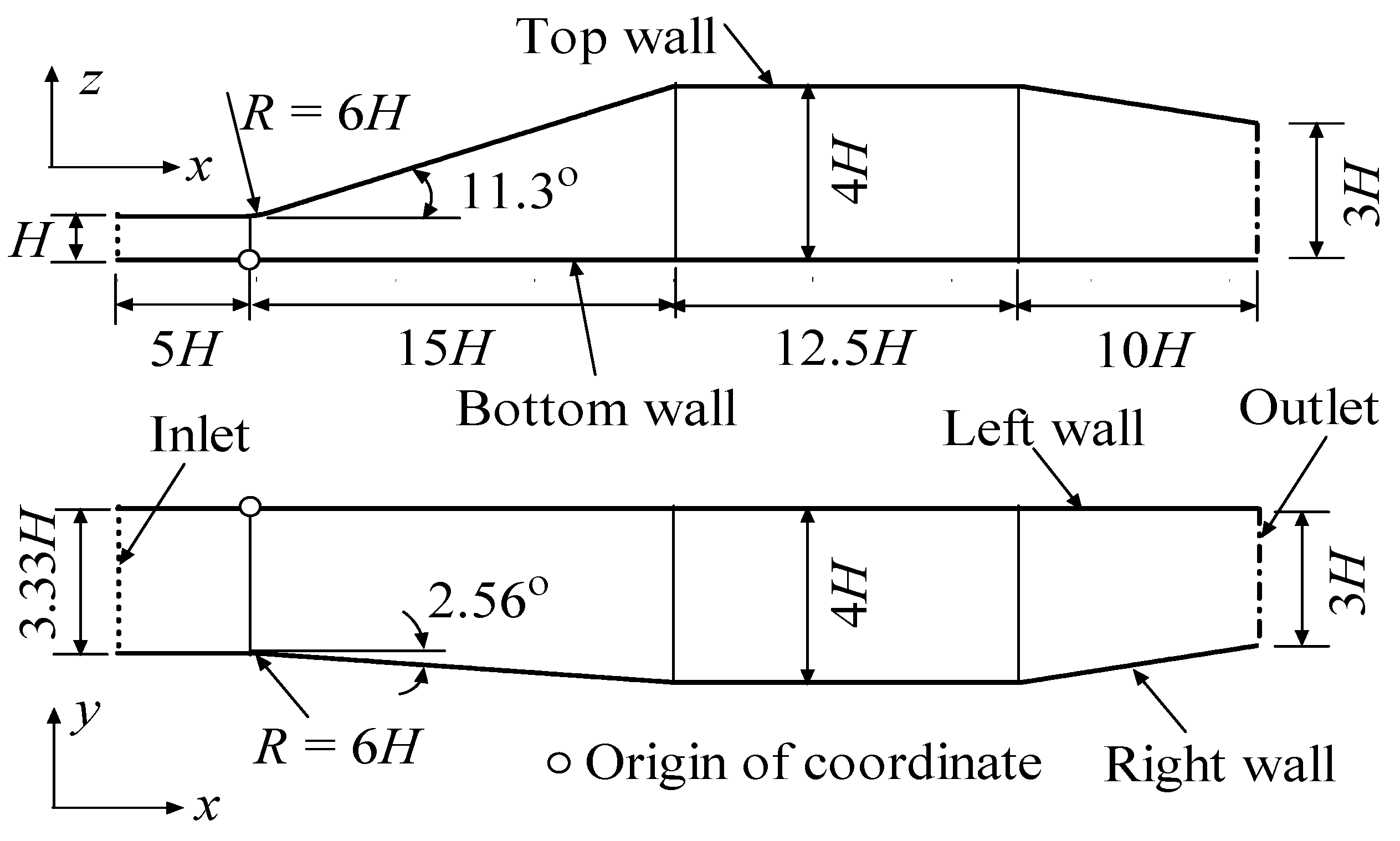
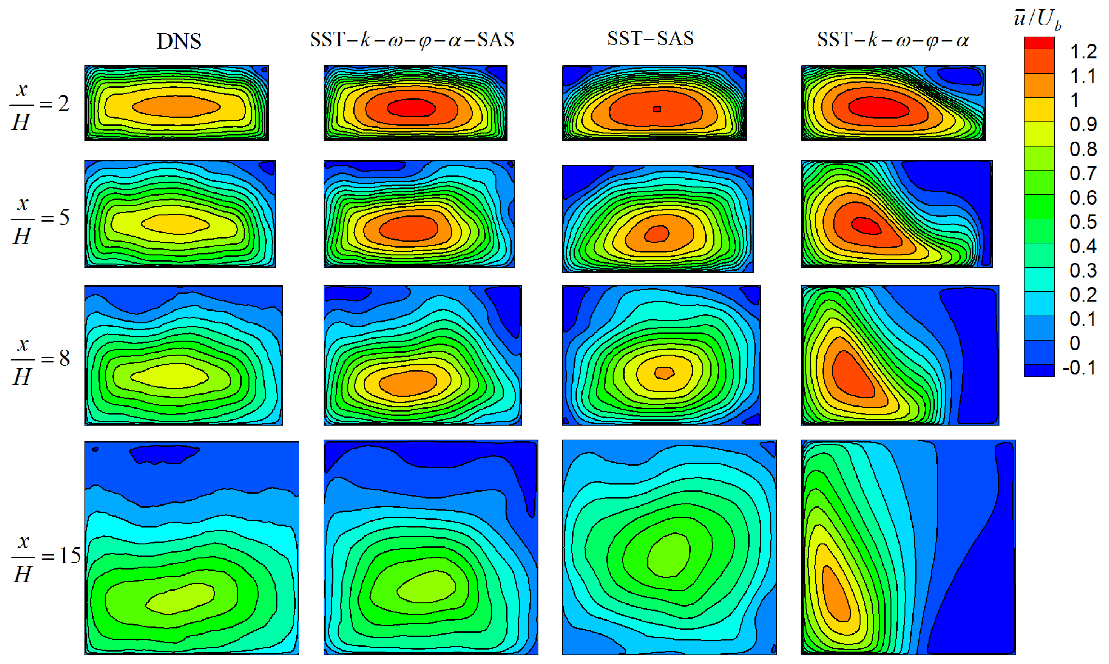
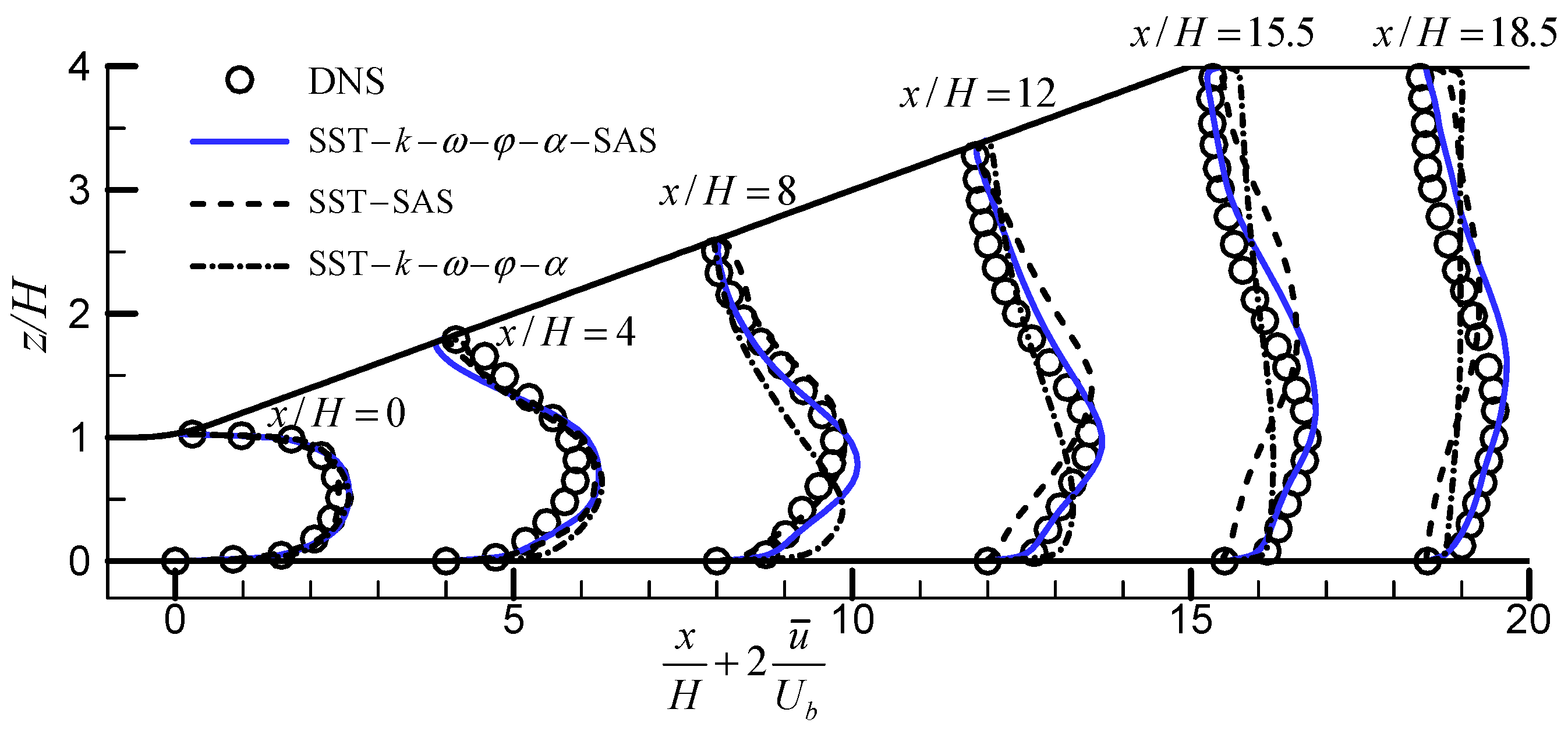
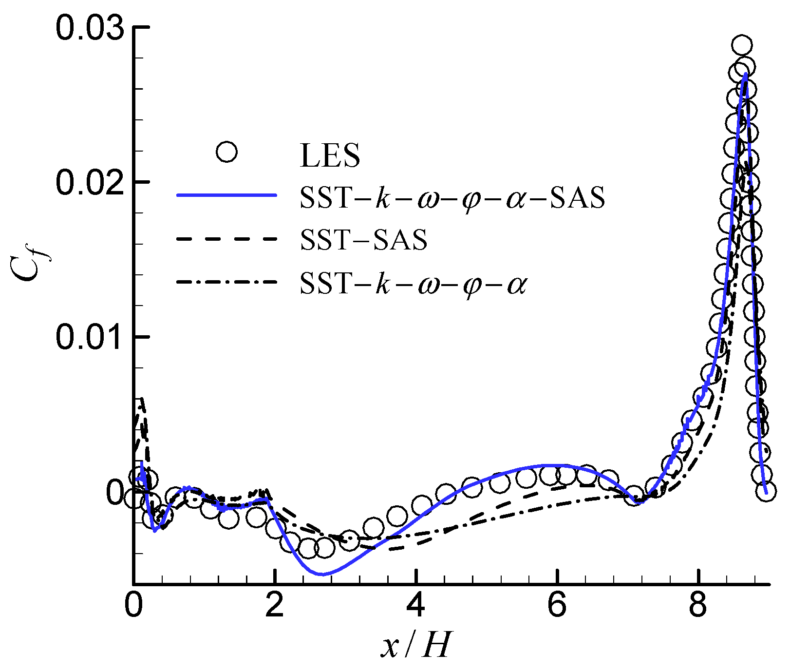
3.3. 2D U-Turn Duct Flow

It is well known that one of the serious weaknesses of conventional eddy viscosity models (EVMs) is that they are unable to capture the effects of strong streamline curvature. To ensure that the EVMs are able to do this, it is usually necessary to make corrections to the models. Several successful solutions have been published to date. For details, readers can refer to Arolla and Durbin [33] and Huang et al. [34]. The 2D U-turn duct flow is challenging for EVMs because of the strong streamline curvature, and it has been a benchmark for assessing the ability of turbulence models. The widely used reference data are the experimental measurements of Monson et al. [35]. For example, York et al. [36] used this flow to test their new eddy viscosity formulation. Smirnov and Menter [37] used this flow to validate the rotation and curvature correction in the SST kω model. Dhakal and Walters [38] used this flow to demonstrate the ability of their three-equation variant of the SST kω model to capture the effect of the streamline curvature.
In contrast to the eddy-viscosity-based RANS models, the LES can predict the strong streamline curvature effects without modifications because the turbulence spectra are resolved. However, the increased computational cost limits its utilization. Hybrid RANS–LES models are worthy of attention as approaches for maintaining a balance between accuracy and efficiency.
The 2D U-turn duct flow was used to test the performance of the proposed SAS model. Figure 10 illustrates the computational model used in this study. In accordance with the experiment of Monson et al. [35], the Re based on the bulk velocity Ub at the inlet and the height of the inlet channel H was 100,000. The domain size in the lateral direction was 4H. The periodic condition was specified in the lateral direction. At the inlet, the fully developed profiles, which were extracted from a preliminary computation in a periodic straight duct at the same Re with the relevant turbulence models, were used. The total number of computational meshes was 5.88 million. The time step size was 0.015H/Ub. The statistics began at 10,000 steps and continued to 30,000 steps to ensure that the mean values of the variables remained unchanged with time.
An arc coordinate (s) was constructed to facilitate the analysis of the results, as shown in Figure 10. A comparison of the mean stream-wise velocity profiles for different transverse sections is shown in Figure 11. It was clearly demonstrated that the two hybrid RANS–LES models (the proposed SAS and SST–SAS models) had a positive effect compared to the RANS model (the SST–kωφα model). At s/H = 0, all three models were able to predict the velocity profile well, and the difference was small. At s/H = π/2, the two hybrid models showed improved results near the concave outer wall compared to the SST–kωφα model, which significantly underpredicted the velocity. At s/H = π, the two hybrid models showed improved results for the entire section. The SST–kωφα model underpredicted the velocity near the concave outer wall and overpredicted the velocity near the convex inner wall. Moreover, in this section, the overall velocity profile predicted by the proposed SAS model was better than that predicted by the SST–SAS model. At s/H = π + 2, the velocity profile predicted by the SST–kωφα model differed dramatically from the experimental results. The velocity near the outer wall predicted by the proposed SAS model matched the experimental results very well, but that near the inner wall differed significantly. It appeared that the SST–kωφα–SAS model overpredicted the separation and slowed down the flow recovery. In contrast, the velocity near the inner wall predicted by the SST–SAS model matched the experimental results very well, but that near the outer wall was underpredicted.
Figure 12 shows the distribution of the Cf along the inner and outer walls near the curved part. The improvement in the results predicted by the two hybrid RANS–LES models was clear. At the inner wall (Figure 12a), the results predicted by the two hybrid RANS–LES models were in good agreement with the experimental results. For the SST–kωφα model, the Cf in the upstream region of the reattachment was well predicted, but the recovery of Cf after separation was significantly delayed. At the outer wall (Figure 12b), the SST–kωφα model failed to predict the peak value of Cf and delayed the recovery of the Cf after separation. The two hybrid RANS–LES models significantly improved the prediction of Cf. Especially for the SST–kωφα–SAS model, the Cf after separation was quite consistent with the experimental results.
It can be seen that, although the baseline model was linear eddy viscosity-based RANS, the hybrid RANS–LES models were indeed able to capture the effect of the strong streamline curvature without any additional correction. This finding is encouraging and expands the application range of hybrid RANS–LES models.

4. Conclusions

An SAS model was developed on the basis of a previously developed elliptic blending-based RANS model. The new SAS model was tested for three cases with boundary layer separation from curved surfaces: 3D diffuser flow, 2D periodic hills flow, and 2D U-turn duct flow. Comparisons of the model predictions with the experimental, DNS, and LES results from the literature, and with the results obtained using the RANS model (SST–kωφα) and another SAS model (SST–SAS) were provided. The following conclusions can be obtained:
(1) In the 3D diffuser flow, the results predicted by the proposed SST–kωφα–SAS model were the best. The SST–kωφα model failed to accurately predict the separation of the flow, leading to incorrect velocity contours and poor pressure distribution. The results predicted by the SST–SAS model were better than those from the SST–kωφα model, but they were quite different from the DNS data.
(2) In the 2D periodic hills flow, the velocity profiles predicted by the proposed SAS and SST–SAS models were in good agreement with LES, but the results of the SST–kωφα model were poor. The length of the recirculation zone predicted by the proposed SAS model was in good agreement with the LES results and was better than that predicted by the SST–SAS model. The SST–kωφα model significantly overpredicted the recirculation length.
(3) In the 2D U-turn duct flow, the two hybrid RANS–LES models had a positive effect compared to the RANS model. The velocity profiles and skin friction were significantly improved.
In summary, the SST–kωφα model could not capture the critical features for all three flows. The SST–SAS model could predict reasonable results. The proposed SAS model was capable of resolving more portions of turbulence structures, and it yielded the best results in all the cases.
The results indicated that the underlying model in the SAS method is very important. Therefore, the development of an advanced RANS model is significant.

Author Contributions

Conceptualization, X.Y. and L.Y.; methodology, X.Y. and L.Y.; software, X.Y.; validation, L.Y.; writing—original draft preparation, X.Y.; writing—review and editing, L.Y. All authors have read and agreed to the published version of the manuscript.

Funding

This research was funded by the National Key R&D Program of China (Grant No. 2018YFB2100901) and the Natural Science Foundation of Shenzhen, China (Grant No. 20200814105851001).

Institutional Review Board Statement

Not applicable.

Informed Consent Statement

Not applicable.

Data Availability Statement

Not applicable.

Conflicts of Interest

The authors declare no conflict of interest.

References

  1. Argyropoulos, C.D.; Markatos, N.C. Recent advances on the numerical modelling of turbulent flows. Appl. Math. Model. 2015, 39, 693–732. [Google Scholar] [CrossRef]
  2. Durbin, P.A. Some Recent Developments in Turbulence Closure Modeling. Annu. Rev. Fluid Mech. 2018, 50, 77–103. [Google Scholar] [CrossRef]
  3. Fröhlich, J.; von Terzi, D. Hybrid LES/RANS methods for the simulation of turbulent flows. Prog. Aerosp. Sci. 2008, 44, 349–377. [Google Scholar] [CrossRef]
  4. Heinz, S. A review of hybrid RANS-LES methods for turbulent flows: Concepts and applications. Prog. Aerosp. Sci. 2020, 114, 100597. [Google Scholar] [CrossRef]
  5. Menter, F.R.; Egorov, Y. The scale-adaptive simulation method for unsteady turbulent flow predictions. Part 1: Theory and model description. Flow Turbul. Combust. 2010, 85, 113–138. [Google Scholar] [CrossRef]
  6. Han, X.; Krajnović, S. Validation of a novel very large eddy simulation method for simulation of turbulent separated flow. Int. J. Numer. Methods Fluids 2013, 73, 436–461. [Google Scholar] [CrossRef]
  7. Durbin, P.A. Near-wall turbulence closure modelling without damping functions. Theor. Comput. Fluid Dyn. 1991, 3, 1–13. [Google Scholar] [CrossRef]
  8. Billard, F.; Laurence, D. A robust k-ε-v2/k elliptic blending turbulence model applied to near-wall, separated and buoyant flows. Int. J. Heat Fluid Flow 2012, 33, 45–58. [Google Scholar] [CrossRef]
  9. Manceau, R. Recent progress in the development of the Elliptic Blending Reynolds-stress model. Int. J. Heat Fluid Flow 2015, 51, 195–220. [Google Scholar] [CrossRef] [Green Version]
  10. Yang, X.L.; Yang, L.; Huang, Z.W.; Liu, Y. Development of a k-ω-φ-α turbulence model based on elliptic blending and applications for near-wall and separated flows. J. Turbul. 2017, 18, 36–60. [Google Scholar] [CrossRef]
  11. Yang, X.L.; Liu, Y. An improved k-ω-φ-α turbulence model applied to near-wall, separated and impinging jet flows and heat transfer. Comput. Math. Appl. 2018, 76, 315–339. [Google Scholar] [CrossRef]
  12. Biswas, R.; Durbin, P.A.; Medic, G. Development of an elliptic blending lag k−ω model. Int. J. Heat Fluid Flow 2019, 76, 26–39. [Google Scholar] [CrossRef]
  13. Shang, W.; Agarwal, R.K. Development and Validation of an Elliptic Blending Lag SST k−ω Turbulence Model. In Proceedings of the AIAA AVIATION 2020 FORUM, Virtual Event, 15–19 June 2020. [Google Scholar] [CrossRef]
  14. Yang, X.L.; Liu, Y.; Yang, L. A shear stress transport incorporated elliptic blending turbulence model applied to near-wall, separated and impinging jet flows and heat transfer. Comput. Math. Appl. 2020, 79, 3257–3271. [Google Scholar] [CrossRef]
  15. Krumbein, B.; Maduta, R.; Jakirlić, S.; Tropea, C. A Scale-Resolving Elliptic-Relaxation-Based Eddy-Viscosity Model: Development and Validation; Springer: Cham, Switzerland, 2020; pp. 90–100. [Google Scholar] [CrossRef]
  16. Hanjalić, K.; Popovac, M.; Hadžiabdić, M. A robust near-wall elliptic-relaxation eddy-viscosity turbulence model for CFD. Int. J. Heat Fluid Flow 2004, 25, 1047–1051. [Google Scholar] [CrossRef]
  17. Menter, F.; Ferreira, J.C.; Esch, T.; Konno, B. The SST turbulence model with improved wall treatment for heat transfer predictions in gas turbines. In Proceedings of the International Gas Turbine Congress, Tokyo, Japan, 2–7 November 2003. [Google Scholar]
  18. Mathey, F.; Cokljat, D.; Bertoglio, J.P.; Sergent, E. Specification of LES inlet boundary conditions using vortex method. In Proceedings of the 4th Internal Symposium, Turbulence, Heat and Mass Transfer, Antalya, Turkey, 12–17 October 2003; pp. 475–482. [Google Scholar]
  19. Cherry, E.M.; Elkins, C.J.; Eaton, J.K. Geometric sensitivity of three-dimensional separated flows. Int. J. Heat Fluid Flow 2008, 29, 803–811. [Google Scholar] [CrossRef]
  20. Cherry, E.M.; Elkins, C.J.; Eaton, J.K. Pressure measurements in a three-dimensional separated diffuser. Int. J. Heat Fluid Flow 2009, 30, 1–2. [Google Scholar] [CrossRef]
  21. Ohlsson, J.; Schlatter, P.; Fischer, P.F.; Henningson, D.S. Direct numerical simulation of separated flow in a three-dimensional diffuser. J. Fluid Mech. 2010, 650, 307–318. [Google Scholar] [CrossRef]
  22. Billard, F.; Revell, A.; Craft, T. Application of recently developed elliptic blending based models to separated flows. Int. J. Heat Fluid Flow 2012, 35, 141–151. [Google Scholar] [CrossRef]
  23. Menter, F.R. Improved two equation k-ω turbulence models for aerodynamic flows. In NASA Technical Memorandum; NASA: Washington, DC, USA, 1992. [Google Scholar]
  24. Speziale, C.G.; Sarkar, S.; Gatski, T.B. Modelling the pressure–strain correlation of turbulence: An invariant dynamical systems approach. J. Fluid Mech. 1991, 227, 245–272. [Google Scholar] [CrossRef]
  25. Manceau, R.; Hanjalić, K. Elliptic blending model: A new near-wall Reynolds-stress turbulence closure. Phys. Fluids 2002, 14, 744–754. [Google Scholar] [CrossRef]
  26. Ohtsuka, T.; Abe, K.-I. An investigation of LES and Hybrid LES/RANS models for predicting 3-D diffuser flow. Int. J. Heat Fluid Flow 2009, 31, 833–844. [Google Scholar] [CrossRef]
  27. Jakirlić, S.; Maduta, R. Extending the bounds of ‘steady’ RANS closures: Toward an instability-sensitive Reynolds stress model. Int. J. Heat Fluid Flow 2015, 51, 175–194. [Google Scholar] [CrossRef]
  28. Temmerman, L.; Leschziner, M. Large eddy simulation of separated flow in a streamwise periodic channel constriction. In 2nd Internatioanl Symposium on Turbulence and Shear Flow Phenomena: Stockholm, Sweden, 2001. In Proceedings of the 2nd Internatioanl Symposium on Turbulence and Shear Flow Phenomena, Stockholm, Sweden, 27–29 June 2001. [Google Scholar]
  29. Fröhlich, J.; Mellen, C.P.; Rodi, W.; Temmerman, L.; Leschziner, M.A. Highly resolved large-eddy simulation of separated flow in a channel with streamwise periodic constrictions. J. Fluid Mech. 2005, 526, 19–66. [Google Scholar] [CrossRef] [Green Version]
  30. Breuer, M.; Peller, N.; Rapp, C.; Manhart, M. Flow over periodic hills–Numerical and experimental study in a wide range of Reynolds numbers. Comput. Fluids 2009, 38, 433–457. [Google Scholar] [CrossRef]
  31. Jang, Y.; Leschziner, M.; Abe, K.; Temmerman, L. Investigation of Anisotropy-Resolving Turbulence Models by Reference to Highly-Resolved LES Data for Separated Flow. Flow Turbul. Combust. 2002, 69, 161–203. [Google Scholar] [CrossRef]
  32. Lien, F.-S.; Kalitzin, G. Computations of transonic flow with the v2–f turbulence model. Int. J. Heat Fluid Flow 2001, 22, 53–61. [Google Scholar] [CrossRef]
  33. Arolla, S.K.; Durbin, P.A. Modeling rotation and curvature effects within scalar eddy viscosity model framework. Int. J. Heat Fluid Flow 2013, 39, 78–89. [Google Scholar] [CrossRef] [Green Version]
  34. Huang, X.; Yang, W.; Li, Y.; Qiu, B.; Guo, Q.; Zhuqing, L. Review on the sensitization of turbulence models to rotation/curvature and the application to rotating machinery. Appl. Math. Comput. 2019, 341, 46–69. [Google Scholar] [CrossRef]
  35. Monson, D.; Seegmiller, H.; McConnaughey, P. Comparison of experiment with calculations using curvature-corrected zero and two equation turbulence models for a two-dimensional U-duct. In Proceedings of the 21st Fluid Dynamics, Plasma Dynamics and Lasers Conference, Seattle, WA, USA, 18–20 June 1990; AIAA: Reston, VA, USA, 1990. AIAA 90–1484. [Google Scholar] [CrossRef]
  36. York, W.D.; Walters, D.K.; Leylek, J.H. A simple and robust linear eddy-viscosity formulation for curved and rotating flows. Int. J. Numer. Methods Heat Fluid Flow 2009, 19, 745–776. [Google Scholar] [CrossRef]
  37. Smirnov, P.E.; Menter, F.R. Sensitization of the SST Turbulence Model to Rotation and Curvature by Applying the Spalart-Shur Correction Term. J. Turbomach. 2009, 131, 041010. [Google Scholar] [CrossRef]
  38. Dhakal, T.P.; Walters, D.K. A Three-Equation Variant of the SST k-ω Model Sensitized to Rotation and Curvature Effects. J. Fluids Eng. 2011, 133, 111201. [Google Scholar] [CrossRef]
Figure 1. Schematic of the geometry and relevant boundary conditions of the 3D diffuser flow.
Applsci 12 02058 g001
Figure 2. The contours of the normalized mean stream-wise velocity at different cross-sections.
Applsci 12 02058 g002
Figure 3. The normalized mean stream-wise velocity profiles on the spanwise midplane.
Applsci 12 02058 g003
Figure 4. The pressure coefficients distributed along the intersection line of the spanwise midplane and the bottom wall.
Applsci 12 02058 g004
Figure 5. Visualization of the turbulent structures using iso-surface of Q = 100 1/s2.
Applsci 12 02058 g005
Figure 6. Schematic of the geometry and boundary conditions of the 2D periodic hills flow.
Applsci 12 02058 g006
Figure 7. Comparison of the normalized mean stream-wise velocity profiles on different transverse sections.
Applsci 12 02058 g007
Figure 8. Comparison of the mean skin friction coefficients distributed along the bottom wall.
Applsci 12 02058 g008
Figure 9. Visualization of the turbulent structures using iso-surface of Q = 30 1/s2.
Applsci 12 02058 g009
Figure 10. Schematic view of the geometry and the boundary conditions for the 2D U-turn flow.
Applsci 12 02058 g010
Figure 11. Comparison of the normalized mean velocity profiles at different transverse sections. (a) s/H = 0; (b) s/H = π/2; (c) s/H = π; (d) s/H = π + 2.
Applsci 12 02058 g011aApplsci 12 02058 g011b
Figure 12. Comparison of the Cf distributed along the curved walls. (a) Inner wall; (b) outer wall.
Applsci 12 02058 g012
Table 1. Locations of separation (Sep.) and reattachment (Reatt.) points and the length of the main recirculation region (Len.) in the 2D periodic hills flow.
ModelSep.Reatt.Len.
LES0.22H4.72H4.50H
SST–kωφα–SAS0.18H4.62H4.44H
SST–SAS0.22H5.79H5.57H
SST–kωφα0.24H7.54H7.30H
Publisher’s Note: MDPI stays neutral with regard to jurisdictional claims in published maps and institutional affiliations.

