
Air Contaminants and Atmospheric Black Carbon Association with White Sky Albedo at Hindukush Karakorum and Himalaya Glaciers


 ,
,
Abstract
:1. Introduction
2. Materials and Methods
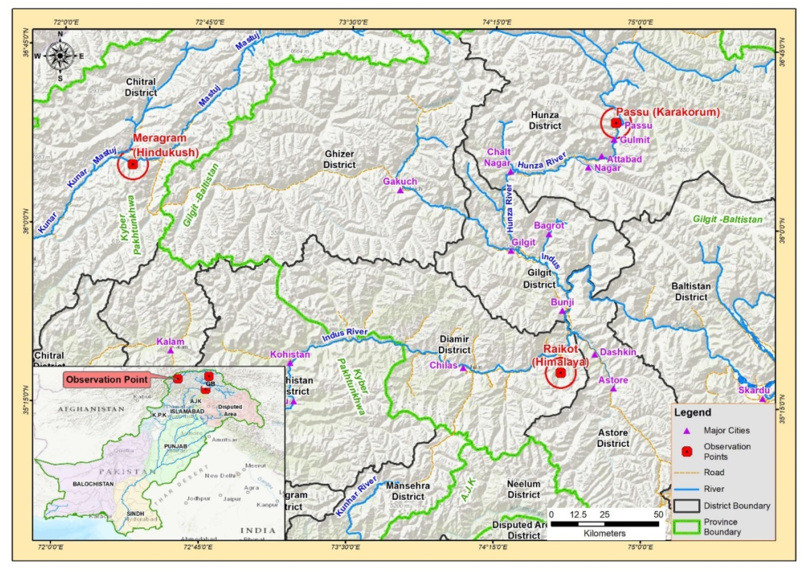
2.1. Study Site
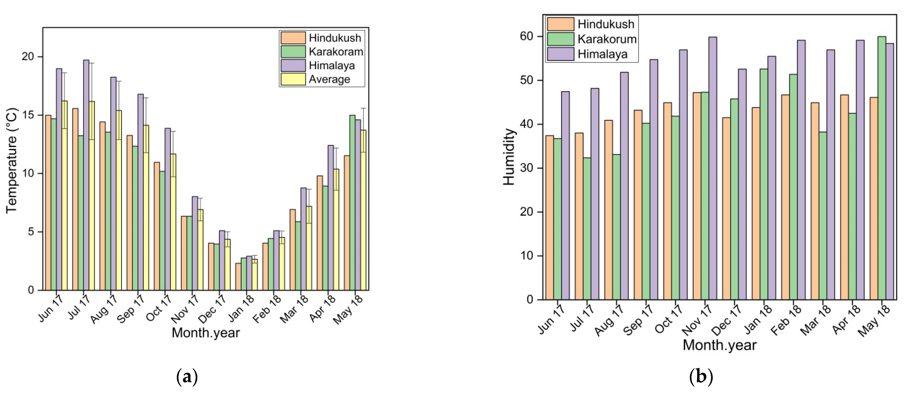
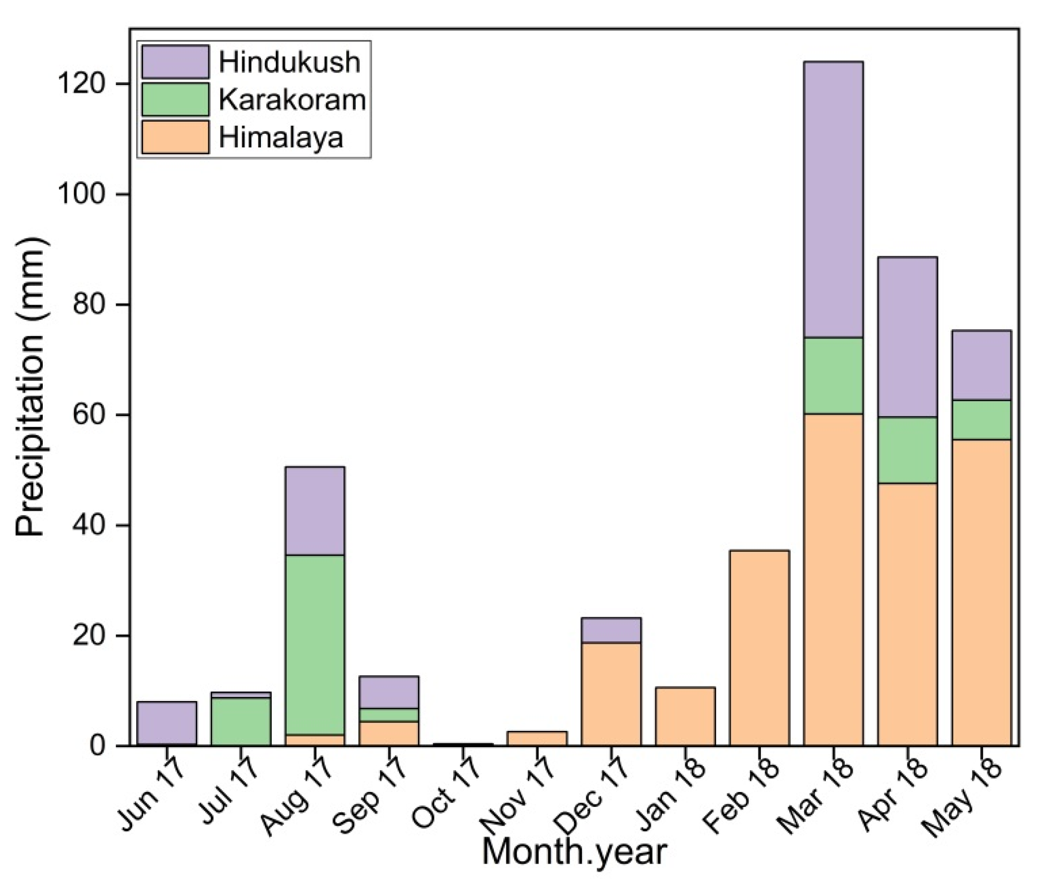
2.2. Temperature, Precipitation, and Humidity
2.3. Work Methodology
2.4. White-Sky Albedo
2.5. Data Analysis
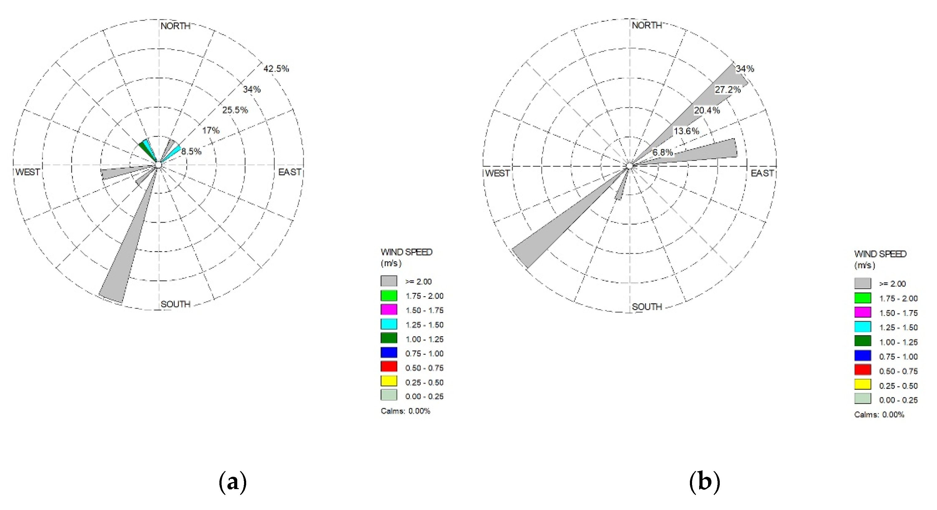
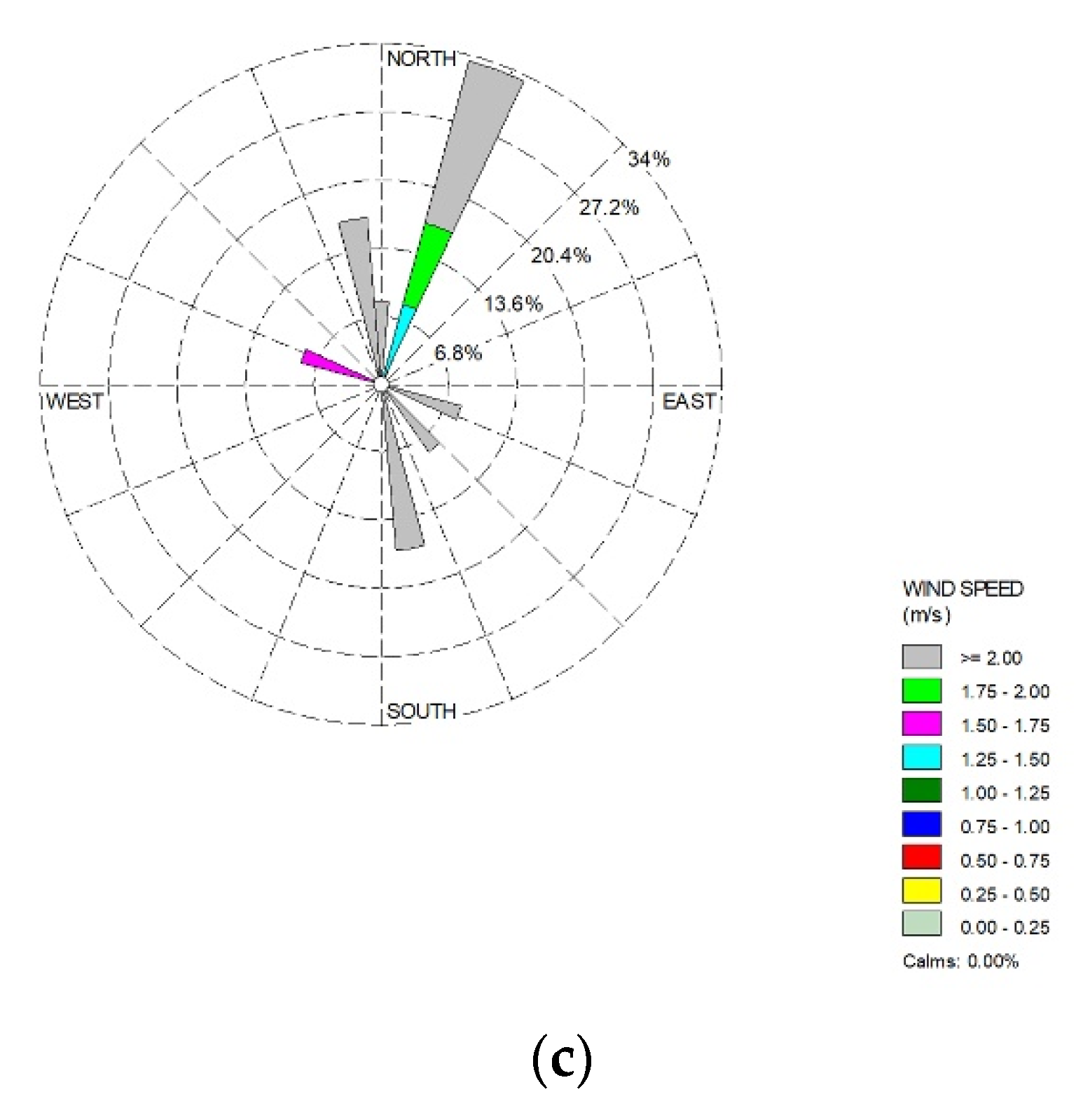
2.6. Wind Plots
3. Results
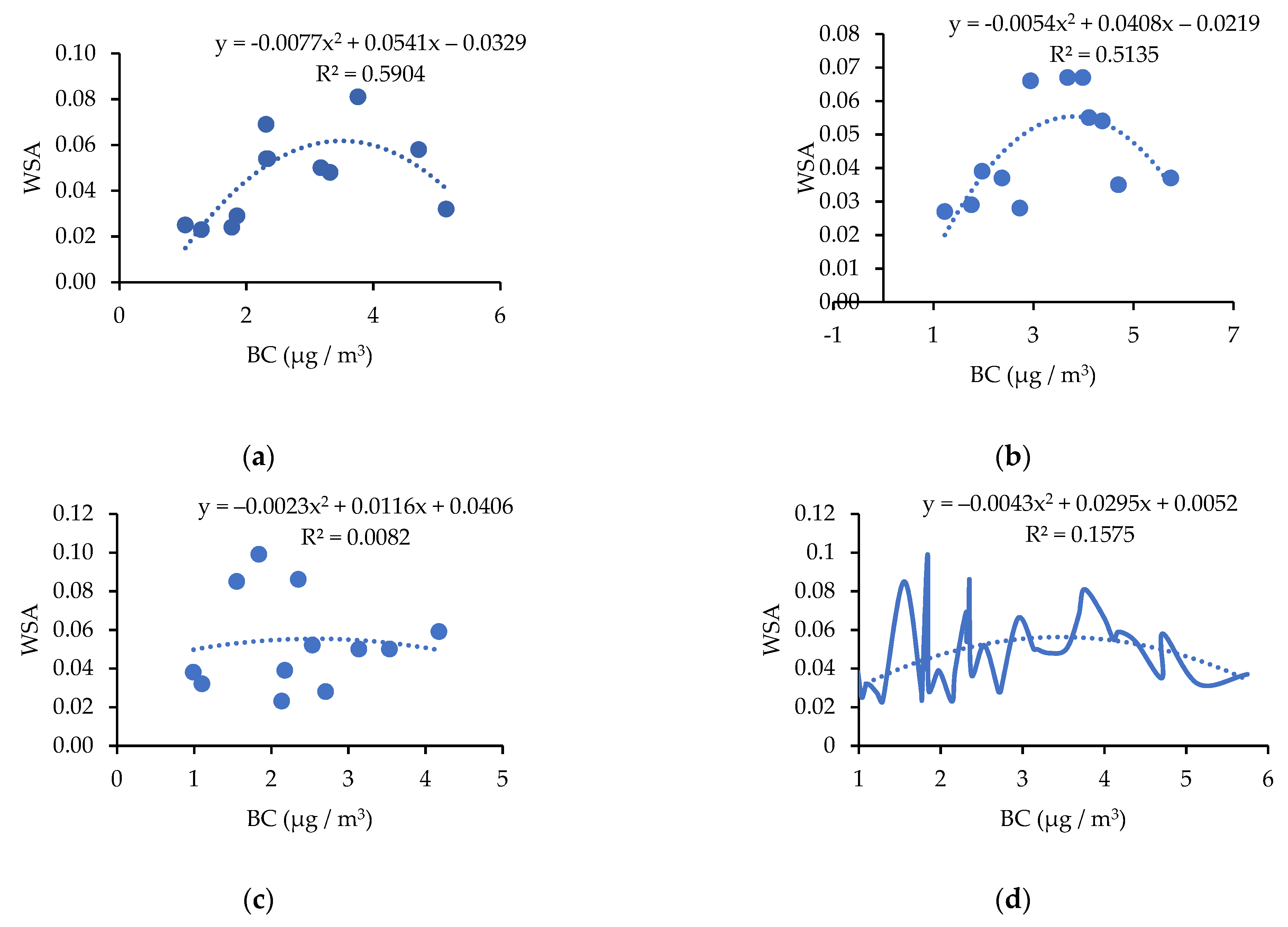
3.1. Black Carbon and White-Sky Albedo
3.2. Wind Trajectories
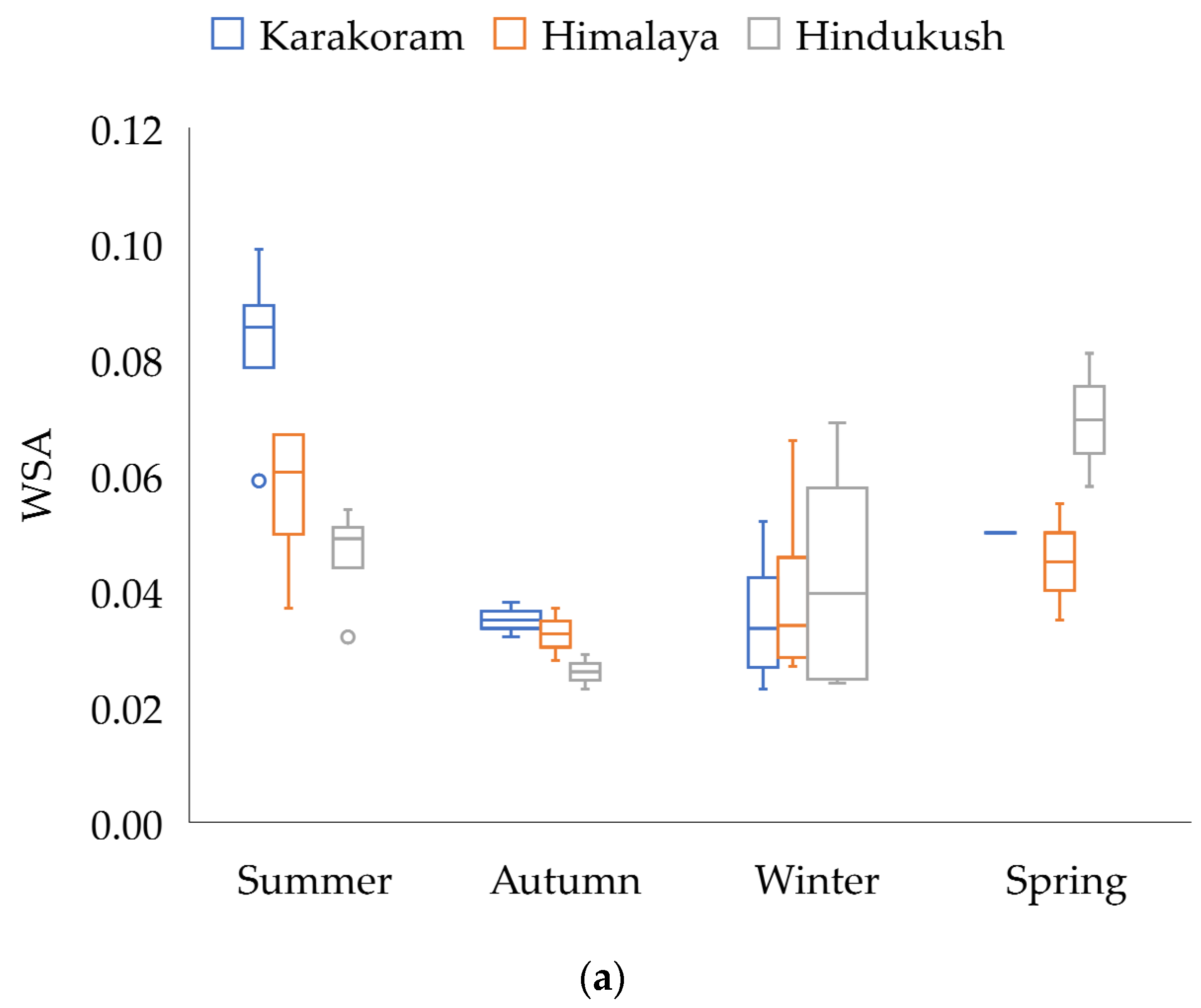
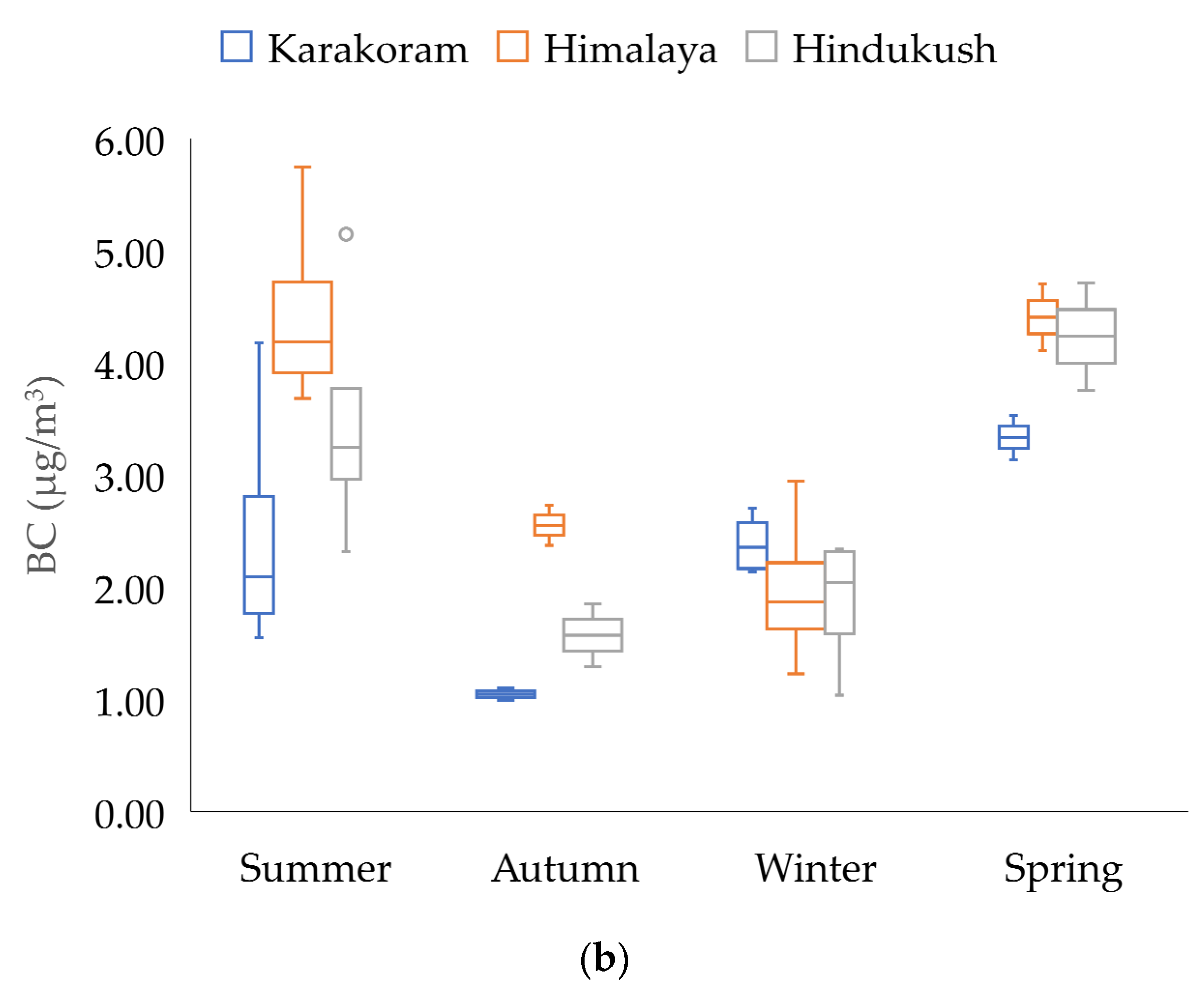
3.3. Box Whisker Plot
4. Discussion
4.1. Effects of Climatic Factors
4.2. Particulate Matter
4.3. Gases Emissions at HKH Glaciers (CO2, NO2, SO2, O3)
4.4. Black Carbon
5. Conclusions
Author Contributions
Funding
Institutional Review Board Statement
Informed Consent Statement
Data Availability Statement
Acknowledgments
Conflicts of Interest
References
- Marzeion, B.; Cogley, J.G.; Richter, K.; Parkes, D. Attribution of global glacier mass loss to anthropogenic and natural causes. Science 2014, 345, 919–921. [Google Scholar] [CrossRef] [PubMed]
- Bolch, T.; Kulkarni, A.; Kääb, A.; Huggel, C.; Paul, F.; Cogley, J.G.; Frey, H.; Kargel, J.S.; Fujita, K.; Scheel, M. The state and fate of Himalayan glaciers. Science 2012, 336, 310–314. [Google Scholar] [CrossRef] [Green Version]
- Brown, M.; Racoviteanu, A.; Tarboton, D.G.; Gupta, A.S.; Nigro, J.; Policelli, F.; Habib, S.; Tokay, M.; Shrestha, M.; Bajracharya, S. An integrated modeling system for estimating glacier and snow melt driven streamflow from remote sensing and earth system data products in the Himalayas. J. Hydrol. 2014, 519, 1859–1869. [Google Scholar] [CrossRef] [Green Version]
- Gurung, D.R.; Giriraj, A.; Aung, K.S.; Shrestha, B.R.; Kulkarni, A.V. Snow-Cover Mapping and Monitoring in the Hindu Kush-Himalayas; International Centre for Integrated Mountain Development (ICIMOD): Patan, Nepal, 2011. [Google Scholar]
- IPCC Intergovernmental Panel on Climate Change. The Physical Science Basis: Contribution of Working Group I to the Fourth Assessment Report of the Intergovernmental Panel on Climate Change. Intergov. Panel Clim. Change 2007, 2007, 996. [Google Scholar]
- Moore, F.C. Climate change and air pollution: Exploring the synergies and potential for mitigation in industrializing countries. Sustainability 2009, 1, 43–54. [Google Scholar] [CrossRef] [Green Version]
- Jacob, D.J. Introduction to Atmospheric Chemistry; Princeton University Press: Princeton, NJ, USA, 1999. [Google Scholar]
- Ramanathan, V.; Carmichael, G. Global and regional climate changes due to black carbon. Nat. Geosci. 2008, 1, 221–227. [Google Scholar] [CrossRef]
- Bond, T.C.; Doherty, S.J.; Fahey, D.W.; Forster, P.M.; Berntsen, T.; DeAngelo, B.J.; Flanner, M.G.; Ghan, S.; Kärcher, B.; Koch, D. Bounding the role of black carbon in the climate system: A scientific assessment. J. Geophys. Res. Atmos. 2013, 118, 5380–5552. [Google Scholar] [CrossRef]
- Beres, N.D.; Lapuerta, M.; Cereceda-Balic, F.; Moosmüller, H. Snow surface albedo sensitivity to black carbon: Radiative transfer modelling. Atmosphere 2020, 11, 1077. [Google Scholar] [CrossRef]
- Beniston, M. Mountain Environments in Changing Climates; Routledge: Oxfordshire, UK, 2002; Volume 59, pp. 5–31. [Google Scholar] [CrossRef]
- Meier, M.F.; Dyurgerov, M.B. How Alaska affects the world. Science 2002, 297, 350–351. [Google Scholar] [CrossRef] [Green Version]
- Haeberli, W.; Hoelzle, M.; Suter, S. Into the second century of worldwide glacier monitoring: Prospects and strategies. J. Hydrol. Reg. Stud. 1998, 56. Available online: https://wgms.ch/downloads/Haeberli_1998.pdf (accessed on 8 July 2020).
- Nakawo, M.; Fujita, K.; Ageta, Y.; Shankar, K.; Pokhrel, A.P. Basic studies for assessing the impacts of the global warming on the Himalayan cryosphere, 1994–1996. Bull. Glaciol. Res. 1997, 15, 53–58. [Google Scholar]
- Molnar, P.; England, P. Late Cenozoic uplift of mountain ranges and global climate change: Chicken or egg? Nature 1990, 346, 29–34. [Google Scholar] [CrossRef]
- Bishop, M.P.; Shroder, J.F., Jr.; Bonk, R.; Olsenholler, J. Geomorphic change in high mountains: A western Himalayan perspective. Glob. Planet. Change 2002, 32, 311–329. [Google Scholar] [CrossRef]
- Dyurgerov, M.B.; Meier, M.F. Twentieth century climate change: Evidence from small glaciers. Proc. Natl. Acad. Sci. USA 2000, 97, 1406–1411. [Google Scholar] [CrossRef] [Green Version]
- Rasul, G.; Chaudhry, Q.; Mahmood, A.; Hyder, K.; Dahe, Q. Glaciers and glacial lakes under changing climate in Pakistan. Pakisan J. Meteorol. 2011, 8, 15. Available online: http://www.climateinfo.pk/frontend/web/attachments/data-type/1_Glaciers%20and%20Glacial%20Lakes%20under%20Changing%20Climate%20in%20Pakistan.pdf (accessed on 8 July 2020).
- Gul, C.; Mahapatra, P.S.; Kang, S.; Singh, P.K.; Wu, X.; He, C.; Kumar, R.; Rai, M.; Xu, Y.; Puppala, S.P. Black carbon concentration in the central Himalayas: Impact on glacier melt and potential source contribution. Environ. Pollut. 2021, 275, 116544. [Google Scholar] [CrossRef] [PubMed]
- Williams, R.S.; Ferrigno, J.G.; Manley, W.F. Glaciers of Asia. In US Geological Survey Professional Paper; USGS: Washington, DC, USA, 2010; p. 349. [Google Scholar]
- Glaciers of Pakistan. Available online: http://www.angelfire.com/al/badela/Glaciers.html (accessed on 20 September 2021).
- Craig, T. Pakistan has more glaciers than almost anywhere on Earth. But they are at risk. The Washington Post, 12 August 2016. [Google Scholar]
- Cogley, G. No ice lost in the Karakoram. Nat. Geosci. 2012, 5, 305–306. [Google Scholar] [CrossRef]
- Kääb, A.; Berthier, E.; Nuth, C.; Gardelle, J.; Arnaud, Y. Contrasting patterns of early twenty-first-century glacier mass change in the Himalayas. Nature 2012, 488, 495–498. [Google Scholar] [CrossRef]
- Jilani, R.H.; Naseer, A.; Paras, S.; Sher, M. Monitoring of Mountain Glacial Variations in Northern Pakistan, from 1992 to 2009 Using Landsat and ALOS data. In Proceedings of the Symposium 4th PI Symposium of JAXA, kyoto, Japan, 15–17 November 2010. [Google Scholar]
- Schmidt, S.; Nüsser, M. Fluctuations of Raikot Glacier during the past 70 years: A case study from the Nanga Parbat massif, northern Pakistan. J. Glaciol. 2009, 55, 949–959. [Google Scholar] [CrossRef] [Green Version]
- Zhang, Y.; Kang, S.; Li, C.; Gao, T.; Cong, Z.; Sprenger, M.; Liu, Y.; Li, X.; Guo, J.; Sillanpää, M. Characteristics of black carbon in snow from Laohugou No. 12 glacier on the northern Tibetan Plateau. Sci. Total Environ. 2017, 607, 1237–1249. [Google Scholar] [CrossRef] [PubMed]
- Worldweather. Available online: worldweatheronline.com (accessed on 31 October 2021). [CrossRef]
- Sarkar, C.; Chatterjee, A.; Singh, A.K.; Ghosh, S.K.; Raha, S. Characterization of black carbon aerosols over Darjeeling-A high altitude Himalayan station in eastern India. Aerosol Air Qual. Res. 2015, 15, 465–478. [Google Scholar] [CrossRef]
- Adak, A.; Chatterjee, A.; Singh, A.K.; Sarkar, C.; Ghosh, S.; Raha, S. Atmospheric fine mode particulates at eastern Himalaya, India: Role of meteorology, long-range transport and local anthropogenic sources. Aerosol Air Qual. Res. 2014, 14, 440–450. [Google Scholar] [CrossRef] [Green Version]
- Stocker, T. Climate Change 2013: The Physical Science Basis: Working Group I Contribution to the Fifth Assessment Report of the Intergovernmental Panel on Climate Change; Cambridge University Press: Cambridge, UK, 2014. [Google Scholar]
- Yao, T.; Xue, Y.; Chen, D.; Chen, F.; Thompson, L.; Cui, P.; Koike, T.; Lau, W.K.-M.; Lettenmaier, D.; Mosbrugger, V. Recent third pole’s rapid warming accompanies cryospheric melt and water cycle intensification and interactions between monsoon and environment: Multidisciplinary approach with observations, modeling, and analysis. Bull. Am. Meteorol. Soc. 2019, 100, 423–444. [Google Scholar] [CrossRef]
- Ghatak, D.; Sinsky, E.; Miller, J. Role of Snow-Albedo Feedback in High Elevation Warming. In Proceedings of the AGU Fall Meeting Abstracts, San Francisco, CA, USA, 10 October 2013; p. A11A-0002. [Google Scholar]
- Zaveri, R.A.; Easter, R.C.; Fast, J.D.; Peters, L.K. Model for simulating aerosol interactions and chemistry (MOSAIC). J. Geophys. Res. Atmos. 2008, 113, D13. [Google Scholar] [CrossRef]
- Sarangi, C.; Qian, Y.; Rittger, K.; Leung, L.R.; Chand, D.; Bormann, K.J.; Painter, T.H. Dust dominates high-altitude snow darkening and melt over high-mountain Asia. Nat. Clim. Chang. 2020, 10, 1045–1051. [Google Scholar] [CrossRef]
- Sun, H.; Liu, X.; Pan, Z. Direct Radiative Effects of Dust Aerosols Emitted from the Tibetan Plateau on the East Asian Summer Monsoon–A Regional Climate Model Simulation. Atmos. Chem. Phys. 2017, 17, 13731–13745. [Google Scholar] [CrossRef] [Green Version]
- Hasnain, S.I. Himalayan glaciers meltdown: Impact on South Asian Rivers. Int. Assoc. Hydrol. Sci. Publ. 2002, 274, 417–423. [Google Scholar] [CrossRef] [Green Version]
- Shen, Y.; Wang, G.; Wu, Q.; Liu, S. The impact of future climate change on ecology and environments in the Changjiang-Yellow Rivers source region. J. Glaciol. Geocryol. 2002, 24, 308–314. [Google Scholar]
- Rai, S.C.; Gurung, T. An Overview of Glaciers, Glacier Retreat, and Subsequent Impacts in Nepal, India and China; ETDEWEB: Washington, DC, USA, 2005. [Google Scholar]
- Chand, D.; Anderson, T.; Wood, R.; Charlson, R.; Hu, Y.; Liu, Z.; Vaughan, M. Quantifying above-cloud aerosol using spaceborne lidar for improved understanding of cloudy-sky direct climate forcing. J. Geophys. Res. Atmos. 2008, 113, D13206. [Google Scholar] [CrossRef] [Green Version]
- Kostrykin, S.; Revokatova, A.; Chernenkov, A.; Ginzburg, V.; Polumieva, P.; Zelenova, M. Black Carbon Emissions from the Siberian Fires 2019: Modelling of the Atmospheric Transport and Possible Impact on the Radiation Balance in the Arctic Region. Atmosphere 2021, 12, 814. [Google Scholar] [CrossRef]
- Ming, J.; Xiao, C.; Cachier, H.; Qin, D.; Qin, X.; Li, Z.; Pu, J. Black Carbon (BC) in the snow of glaciers in west China and its potential effects on albedos. Atmos. Res. 2009, 92, 114–123. [Google Scholar] [CrossRef]
- Yang, S.; Xu, B.; Cao, J.; Zender, C.S.; Wang, M. Climate effect of black carbon aerosol in a Tibetan Plateau glacier. Atmos. Environ. 2015, 111, 71–78. [Google Scholar] [CrossRef] [Green Version]
- Ming, J.; Xiao, C.; Du, Z.; Yang, X. An overview of black carbon deposition in High Asia glaciers and its impacts on radiation balance. Adv. Water Resour. 2013, 55, 80–87. [Google Scholar] [CrossRef]
- Ruppel, M.; Isaksson, E.; Ström, J.; Beaudon, E.; Svensson, J.; Pedersen, C.; Korhola, A. Increase in elemental carbon values between 1970 and 2004 observed in a 300-year ice core from Holtedahlfonna (Svalbard). Atmos. Chem. Phys. 2014, 14, 11447–11460. [Google Scholar] [CrossRef] [Green Version]
- Aoki, T.; Matoba, S.; Yamaguchi, S.; Tanikawa, T.; Niwano, M.; Kuchiki, K.; Adachi, K.; Uetake, J.; Motoyama, H.; Hori, M. Light-absorbing snow impurity concentrations measured on Northwest Greenland ice sheet in 2011 and 2012. Bull. Glaciol. Res. 2014, 32, 21–31. [Google Scholar] [CrossRef] [Green Version]
- Thevenon, F.; Anselmetti, F.S.; Bernasconi, S.M.; Schwikowski, M. Mineral dust and elemental black carbon records from an Alpine ice core (Colle Gnifetti glacier) over the last millennium. J. Geophys. Res. Atmos. 2009, 114, D17. [Google Scholar] [CrossRef] [Green Version]
- Clark, D. Emission Factors for Black Carbon; Cundall Johnston & Partners LLP: Newcastle, UK, 2013. [Google Scholar]
- Kaspari, S.; Painter, T.H.; Gysel, M.; Skiles, S.; Schwikowski, M. Seasonal and elevational variations of black carbon and dust in snow and ice in the Solu-Khumbu, Nepal and estimated radiative forcings. Atmos. Chem. Phys. 2014, 14, 8089–8103. [Google Scholar] [CrossRef]
- Qu, B.; Ming, J.; Kang, S.-C.; Zhang, G.-S.; Li, Y.-W.; Li, C.-D.; Zhao, S.-Y.; Ji, Z.-M.; Cao, J.-J. The decreasing albedo of the Zhadang glacier on western Nyainqentanglha and the role of light-absorbing impurities. Atmos. Chem. Phys. 2014, 14, 11117–11128. [Google Scholar] [CrossRef] [Green Version]
- Xu, B.; Cao, J.; Hansen, J.; Yao, T.; Joswia, D.R.; Wang, N.; Wu, G.; Wang, M.; Zhao, H.; Yang, W. Black soot and the survival of Tibetan glaciers. Proc. Natl. Acad. Sci. USA 2009, 106, 22114–22118. [Google Scholar] [CrossRef] [PubMed] [Green Version]
- Gertler, C.G.; Puppala, S.P.; Panday, A.; Stumm, D.; Shea, J. Black carbon and the Himalayan cryosphere: A review. Atmos. Environ. 2016, 125, 404–417. [Google Scholar] [CrossRef]
- Ming, J.; Cachier, H.; Xiao, C.; Qin, D.; Kang, S.; Hou, S.; Xu, J. Black carbon record based on a shallow Himalayan ice core and its climatic implications. Atmos. Chem. Phys. 2008, 8, 1343–1352. [Google Scholar] [CrossRef] [Green Version]
- Bond, T.C.; Streets, D.G.; Yarber, K.F.; Nelson, S.M.; Woo, J.H.; Klimont, Z. A technology-based global inventory of black and organic carbon emissions from combustion. J. Geophys. Res. Atmos. 2004, 109. [Google Scholar] [CrossRef] [Green Version]
- Dumont, M.; Brun, E.; Picard, G.; Michou, M.; Libois, Q.; Petit, J.; Geyer, M.; Morin, S.; Josse, B. Contribution of light-absorbing impurities in snow to Greenland’s darkening since 2009. Nat. Geosci. 2014, 7, 509–512. [Google Scholar] [CrossRef]
- Flanner, M.G.; Zender, C.S.; Randerson, J.T.; Rasch, P.J. Present-day climate forcing and response from black carbon in snow. J. Geophys. Res. Atmos. 2007, 112, D11202. [Google Scholar] [CrossRef] [Green Version]
- Lau, W.K.; Kim, M.-K.; Kim, K.-M.; Lee, W.-S. Enhanced surface warming and accelerated snow melt in the Himalayas and Tibetan Plateau induced by absorbing aerosols. Environ. Res. Lett. 2010, 5, 25204. [Google Scholar] [CrossRef]
- Yasunari, T.; Bonasoni, P.; Laj, P.; Fujita, K.; Vuillermoz, E.; Marinoni, A.; Cristofanelli, P.; Duchi, R.; Tartari, G.; Lau, K.-M. Estimated impact of black carbon deposition during pre-monsoon season from Nepal Climate Observatory–Pyramid data and snow albedo changes over Himalayan glaciers. Atmos. Chem. Phys. 2010, 10, 6603–6615. [Google Scholar] [CrossRef] [Green Version]
- Gustafsson, Ö.; Ramanathan, V. Convergence on climate warming by black carbon aerosols. Proc. Natl. Acad. Sci. USA 2016, 113, 4243–4245. [Google Scholar] [CrossRef] [Green Version]
- Ji, Z.; Kang, S.C.; Cong, Z.Y.; Zhang, Q.G.; Yao, T.D. 2015: Simulation of carbonaceous aerosols over the Third Pole and adjacent regions: Distribution, transportation, deposition, and climatic effects. Clim. Dyn. 2015, 45, 2831–2846. [Google Scholar] [CrossRef]
- Qian, Y.; Yasunari, T.J.; Doherty, S.J.; Flanner, M.G.; Lau, W.K.; Ming, J.; Wang, H.; Wang, M.; Warren, S.G.; Zhang, R. Light-absorbing particles in snow and ice: Measurement and modeling of climatic and hydrological impact. Adv. Atmos. Sci. 2015, 32, 64–91. [Google Scholar] [CrossRef]
- Wild, M.; Folini, D.; Schär, C.; Loeb, N.; König-Langlo, G. Earth Radiation Balance as Observed and Represented in CMIP5 models. In Proceedings of the EGU General Assembly Conference Abstracts, Vienna, Austria, 27 April–2 May 2014; p. 7867. [Google Scholar]
- Xu, Y.; Ramanathan, V.; Washington, W. Observed high-altitude warming and snow cover retreat over Tibet and the Himalayas enhanced by black carbon aerosols. Atmos. Chem. Phys. 2016, 16, 1303–1315. [Google Scholar] [CrossRef] [Green Version]
- Yasunari, T.J.; Tan, Q.; Lau, K.-M.; Bonasoni, P.; Marinoni, A.; Laj, P.; Ménégoz, M.; Takemura, T.; Chin, M. Estimated range of black carbon dry deposition and the related snow albedo reduction over Himalayan glaciers during dry pre-monsoon periods. Atmos. Environ. 2013, 78, 259–267. [Google Scholar] [CrossRef]
- Fujita, K.-I.; Maeda, D.; Xiao, Q.; Srinivasula, S.M. Nrf2-mediated induction of p62 controls Toll-like receptor-4–driven aggresome-like induced structure formation and autophagic degradation. Proc. Natl. Acad. Sci. USA 2011, 108, 1427–1432. [Google Scholar] [CrossRef] [Green Version]
- Benning, L.G.; Anesio, A.M.; Lutz, S.; Tranter, M. Biological impact on Greenland’s albedo. Nat. Geosci. 2014, 7, 691. [Google Scholar] [CrossRef]
- Uetake, J.; Naganuma, T.; Hebsgaard, M.B.; Kanda, H.; Kohshima, S. Communities of algae and cyanobacteria on glaciers in west Greenland. Polar. Sci. 2010, 4, 71–80. [Google Scholar] [CrossRef] [Green Version]
- Yallop, M.L.; Anesio, A.M.; Perkins, R.G.; Cook, J.; Telling, J.; Fagan, D.; MacFarlane, J.; Stibal, M.; Barker, G.; Bellas, C. Photophysiology and albedo-changing potential of the ice algal community on the surface of the Greenland ice sheet. ISME J. 2012, 6, 2302–2313. [Google Scholar] [CrossRef] [Green Version]


| Hindukush (R²) | Karakoram (R²) | Himalaya (R²) | Cumulative (R²) |
|---|---|---|---|
| 0.5904 | 0.0082 | 0.5135 | 0.1575 |
| Year | Hindukush (Meragram) | Karakoram (Passu) | Himalaya (Raikot) | |||
|---|---|---|---|---|---|---|
| Wind Speed (m/s) | Wind Direction | Wind Speed (m/s) | Wind Direction | Wind Speed (m/s) | Wind Direction | |
| Jun-17 | 2.50 | NNW | 1.39 | NNW | 3.33 | ENE |
| Jul-17 | 1.66 | WNW | 1.11 | NW | 5.00 | ENE |
| Aug-17 | 2.50 | NNW | 1.39 | NE | 3.05 | NE |
| Sep-17 | 2.22 | NNE | 2.22 | ENE | 3.89 | NE |
| Oct-17 | 3.89 | SE | 4.17 | SSW | 3.89 | NE |
| Nov-17 | 1.94 | NNE | 3.33 | SSW | 3.89 | ENE |
| Dec-17 | 2.78 | SSE | 5.83 | SSW | 3.61 | NE |
| Jan-18 | 3.61 | SSE | 9.73 | WSW | 3.61 | SW |
| Feb-18 | 2.22 | ENE | 3.61 | SSW | 4.17 | SSW |
| Mar-18 | 3.33 | NNE | 3.05 | SSW | 5.00 | SW |
| Apr-18 | 3.05 | N | 2.78 | WSW | 3.89 | SW |
| May-18 | 1.39 | NNE | 2.78 | SW | 3.89 | SW |
| Gases | Sites | Jun-17 | Jul-17 | Aug-17 | Sep-17 | Oct-17 | Nov-17 | Dec-17 | Jan-18 | Feb-18 | Mar-18 | Apr-18 | May-18 | Mean | SD |
|---|---|---|---|---|---|---|---|---|---|---|---|---|---|---|---|
| O3 (µg/m3) | Hindukush | 24.22 | 28.84 | 31.14 | 29.99 | 28.84 | 27.68 | 24.80 | 22.49 | 21.91 | 24.22 | 23.07 | 25.95 | 26.10 | 3.11 |
| Karakorum | 23.74 | 24.51 | 25.09 | 27.89 | 26.82 | 27.68 | 21.48 | 26.99 | 24.11 | 20.59 | 20.99 | 33.74 | 25.30 | 3.68 | |
| Himalaya | 30.66 | 36.50 | 39.42 | 37.96 | 36.50 | 35.04 | 31.39 | 28.47 | 27.74 | 30.66 | 29.20 | 32.85 | 33.03 | 3.94 | |
| CO2 ppm | Hindukush | 153.40 | 216.84 | 211.07 | 149.37 | 155.13 | 213.96 | 205.31 | 206.46 | 200.11 | 195.50 | 199.54 | 197.23 | 191.99 | 24.64 |
| Karakorum | 150.33 | 184.31 | 188.65 | 138.91 | 144.27 | 213.96 | 196.11 | 247.75 | 220.13 | 166.18 | 181.58 | 256.40 | 190.72 | 38.38 | |
| Himalaya | 194.18 | 274.48 | 267.18 | 189.07 | 196.37 | 270.83 | 259.88 | 261.34 | 253.31 | 247.47 | 252.58 | 249.66 | 243.03 | 31.19 | |
| SO2 ppm | Hindukush | 1.53 | 1.28 | 1.41 | 1.27 | 1.26 | 1.72 | 1.85 | 1.99 | 1.86 | 1.70 | 1.64 | 1.56 | 1.59 | 0.25 |
| Karakorum | 1.50 | 1.09 | 1.11 | 1.19 | 1.17 | 1.72 | 1.83 | 2.39 | 2.05 | 1.45 | 1.50 | 2.03 | 1.58 | 0.42 | |
| Himalaya | 1.93 | 1.62 | 1.79 | 1.61 | 1.59 | 2.18 | 2.34 | 2.52 | 2.36 | 2.15 | 2.08 | 1.98 | 2.01 | 0.31 | |
| NO2 ppm | Hindukush | 2.68 | 2.79 | 2.43 | 2.05 | 2.18 | 2.80 | 2.83 | 2.86 | 2.84 | 2.80 | 2.46 | 2.53 | 2.60 | 0.27 |
| Karakorum | 2.63 | 2.37 | 2.42 | 1.91 | 2.03 | 2.80 | 2.79 | 3.43 | 3.13 | 2.38 | 2.24 | 3.29 | 2.62 | 0.49 | |
| Himalaya | 3.39 | 3.53 | 3.07 | 2.60 | 2.76 | 3.55 | 3.58 | 3.62 | 3.60 | 3.54 | 3.12 | 3.20 | 3.30 | 0.35 |
| Pollutants | Site | Jun-17 | Jul-17 | Aug-17 | Sep-17 | Oct-17 | Nov-17 | Dec-17 | Jan-18 | Feb-18 | Mar-18 | Apr-18 | May-18 | Mean | SD |
|---|---|---|---|---|---|---|---|---|---|---|---|---|---|---|---|
| PM 2.5 (µg/m3) | Hindukush | 15.57 | 17.88 | 13.84 | 13.84 | 12.69 | 15.57 | 20.18 | 19.03 | 12.11 | 11.53 | 12.69 | 12.11 | 14.75 | 2.91 |
| Karakorum | 15.26 | 15.20 | 15.55 | 12.87 | 11.80 | 15.57 | 11.87 | 22.84 | 13.32 | 9.80 | 11.55 | 15.74 | 14.28 | 3.34 | |
| Himalaya | 19.71 | 22.63 | 17.52 | 17.52 | 16.06 | 19.71 | 25.55 | 24.09 | 15.33 | 14.60 | 16.06 | 15.33 | 18.68 | 3.69 | |
| PM 10 (µg/m3) | Hindukush | 23.64 | 28.84 | 25.95 | 24.22 | 23.64 | 28.26 | 28.26 | 28.26 | 24.80 | 24.22 | 25.37 | 24.80 | 25.86 | 2.00 |
| Karakorum | 23.17 | 24.51 | 25.09 | 22.53 | 21.99 | 28.26 | 24.30 | 33.91 | 27.28 | 20.59 | 23.09 | 32.24 | 25.58 | 4.11 | |
| Himalaya | 29.93 | 36.50 | 32.85 | 30.66 | 29.93 | 35.77 | 35.77 | 35.77 | 31.39 | 30.66 | 32.12 | 31.39 | 32.73 | 2.53 | |
| TSP (µg/m3) | Hindukush | 67.84 | 80.81 | 68.84 | 65.85 | 62.85 | 75.82 | 83.81 | 81.81 | 63.85 | 61.86 | 65.85 | 63.85 | 70.25 | 8.05 |
| Karakorum | 66.49 | 68.69 | 70.31 | 61.24 | 58.45 | 75.82 | 62.58 | 98.17 | 70.24 | 52.58 | 59.92 | 83.01 | 68.96 | 12.32 | |
| Himalaya | 85.88 | 102.29 | 87.14 | 83.35 | 79.56 | 95.98 | 106.08 | 103.56 | 80.83 | 78.30 | 83.35 | 80.83 | 88.93 | 10.20 |
| Black Carbon | Site | Jun-17 | Jul-17 | Aug-17 | Sep-17 | Oct-17 | Nov-17 | Dec-17 | Jan-18 | Feb-18 | Mar-18 | Apr-18 | May-18 | Mean | SD |
|---|---|---|---|---|---|---|---|---|---|---|---|---|---|---|---|
| BC River Water µg/m3 | Hindukush | 80.46 | 83.28 | 105.84 | 90.80 | 71.41 | 75.61 | 80.23 | 61.83 | 94.90 | 118.17 | 82.09 | 44.58 | 82.43 | 19.27 |
| Karakorum | 78.85 | 70.78 | 72.45 | 84.45 | 66.41 | 75.61 | 93.00 | 74.19 | 104.39 | 100.45 | 74.70 | 57.95 | 79.44 | 13.79 | |
| Himalaya | 101.84 | 105.41 | 133.98 | 114.94 | 90.39 | 95.72 | 101.55 | 78.26 | 120.13 | 149.58 | 103.91 | 56.43 | 104.34 | 24.40 | |
| BC Glacier µg/m3 | Hindukush | 14.61 | 14.46 | 14.69 | 14.82 | 15.32 | 15.75 | 15.90 | 15.97 | 16.53 | 16.17 | 16.24 | 15.58 | 15.50 | 0.71 |
| Karakorum | 14.32 | 14.81 | 15.16 | 16.21 | 15.37 | 17.44 | 16.39 | 15.62 | 16.35 | 16.72 | 15.44 | 14.41 | 15.69 | 0.96 | |
| Himalaya | 21.41 | 22.52 | 21.56 | 22.92 | 20.48 | 21.29 | 22.83 | 22.41 | 22.11 | 21.89 | 21.34 | 20.82 | 21.80 | 0.78 | |
| BC Snow/Rain (ng/g) mass | Hindukush | 51.62 | 54.44 | 77.01 | 61.97 | 42.57 | 46.78 | 51.39 | 32.99 | 66.07 | 89.34 | 53.25 | 15.74 | 53.60 | 19.27 |
| Karakorum | 50.59 | 46.27 | 47.36 | 57.63 | 39.59 | 46.78 | 64.74 | 39.59 | 72.67 | 75.94 | 48.46 | 20.46 | 50.84 | 15.31 | |
| Himalaya | 65.34 | 68.91 | 97.48 | 78.44 | 53.89 | 59.22 | 65.05 | 41.76 | 83.63 | 113.08 | 67.41 | 19.93 | 67.84 | 24.40 |
| Month | Hindukush (Meragram) | Karakoram (Passu) | Himalaya (Raikot) | ||||||
|---|---|---|---|---|---|---|---|---|---|
| BC µg/m3 | WSA | Cloud Cover (%) | BC µg/m3 | WSA * | Cloud Cover (%) | BC µg/m3 | WSA | Cloud Cover (%) | |
| Jun-17 | 3.32 | 0.048 | 2 | 2.35 | 0.086 | 11 | 0.054 | 0.044 | 11 |
| Jul-17 | 3.18 | 0.050 | 4 | 1.84 | 0.099 | 18 | 0.067 | 0.050 | 18 |
| Aug-17 | 2.32 | 0.054 | 5 | 1.55 | 0.085 | 32 | 0.067 | 0.051 | 4 |
| Sep-17 | 1.85 | 0.029 | 5 | 0.99 | 0.038 | 61 | 0.037 | 0.030 | 2 |
| Oct-17 | 1.29 | 0.023 | 5 | 1.10 | 0.032 | 6 | 0.028 | 0.022 | 0 |
| Nov-17 | 1.04 | 0.025 | 50 | 2.71 | 0.028 | 29 | 0.029 | 0.023 | 30 |
| Dec-17 | 1.77 | 0.024 | 43 | 2.14 | 0.023 | 11 | 0.027 | 0.052 | 49 |
| Jan-18 | 2.31 | 0.069 | 47 | 2.18 | 0.039 | 10 | 0.039 | 0.064 | 17 |
| Feb-18 | 2.34 | 0.054 | 47 | 2.53 | 0.052 | 4 | 0.066 | 0.061 | 61 |
| Mar-18 | 3.76 | 0.081 | 32 | 3.14 | 0.050 | 6 | 0.055 | 0.071 | 59 |
| Apr-18 | 4.71 | 0.058 | 3 | 3.53 | 0.050 | 2 | 0.035 | 0.054 | 2 |
| May-18 | 5.15 | 0.032 | 17 | 4.18 | 0.059 | 43 | 0.037 | 0.034 | 29 |
| Mean | 2.752 | 0.0456 | 21.667 | 2.3531 | 0.0534 | 19.417 | 3.3018 | 0.0451 | 23.500 |
| Range | 4.109 | 0.040 | 48.000 | 3.1857 | 0.076 | 59.000 | 4.5196 | 0.058 | 61.000 |
| S.D | 1.296 | 0.019 | 20.340 | 0.9483 | 0.0246 | 18.263 | 1.3527 | 0.0157 | 22.310 |
| Variance | 1.681 | 0.0002 | 413.697 | 0.8993 | 0.0006 | 333.538 | 1.8299 | 0.0004 | 497.727 |
| Maximum | 5.146 | 0.081 | 50.000 | 4.1765 | 0.099 | 61.000 | 5.7474 | 0.067 | 61.000 |
| Minimum | 1.037 | 0.0230 | 2.000 | 0.9908 | 0.0230 | 2.000 | 1.2279 | 0.0270 | 0.000 |
Publisher’s Note: MDPI stays neutral with regard to jurisdictional claims in published maps and institutional affiliations. |
© 2022 by the authors. Licensee MDPI, Basel, Switzerland. This article is an open access article distributed under the terms and conditions of the Creative Commons Attribution (CC BY) license (https://creativecommons.org/licenses/by/4.0/).
Share and Cite
Zainab, I.; Ali, Z.; Ahmad, U.; Raza, S.T.; Ahmad, R.; Zona, Z.; Sidra, S. Air Contaminants and Atmospheric Black Carbon Association with White Sky Albedo at Hindukush Karakorum and Himalaya Glaciers. Appl. Sci. 2022, 12, 962. https://doi.org/10.3390/app12030962
Zainab I, Ali Z, Ahmad U, Raza ST, Ahmad R, Zona Z, Sidra S. Air Contaminants and Atmospheric Black Carbon Association with White Sky Albedo at Hindukush Karakorum and Himalaya Glaciers. Applied Sciences. 2022; 12(3):962. https://doi.org/10.3390/app12030962
Chicago/Turabian StyleZainab, Irfan, Zulfiqar Ali, Usman Ahmad, Syed Turab Raza, Rida Ahmad, Zaidi Zona, and Safdar Sidra. 2022. "Air Contaminants and Atmospheric Black Carbon Association with White Sky Albedo at Hindukush Karakorum and Himalaya Glaciers" Applied Sciences 12, no. 3: 962. https://doi.org/10.3390/app12030962