
Self-Supervised Noise Reduction in Low-Dose Cone Beam Computed Tomography (CBCT) Using the Randomly Dropped Projection Strategy


Abstract
:1. Introduction
- We define a self-supervised denoising scheme that solves the problems of noise reduction in the projection image domain and reconstructed image domain in LDCT;
- We propose a neural network that can be trained on a small number of training samples and can yield promising results;
- The proposed method exhibits solid performance improvement compared with the existing self-supervised noise reduction methods.
2. Related Works
3. Methodology
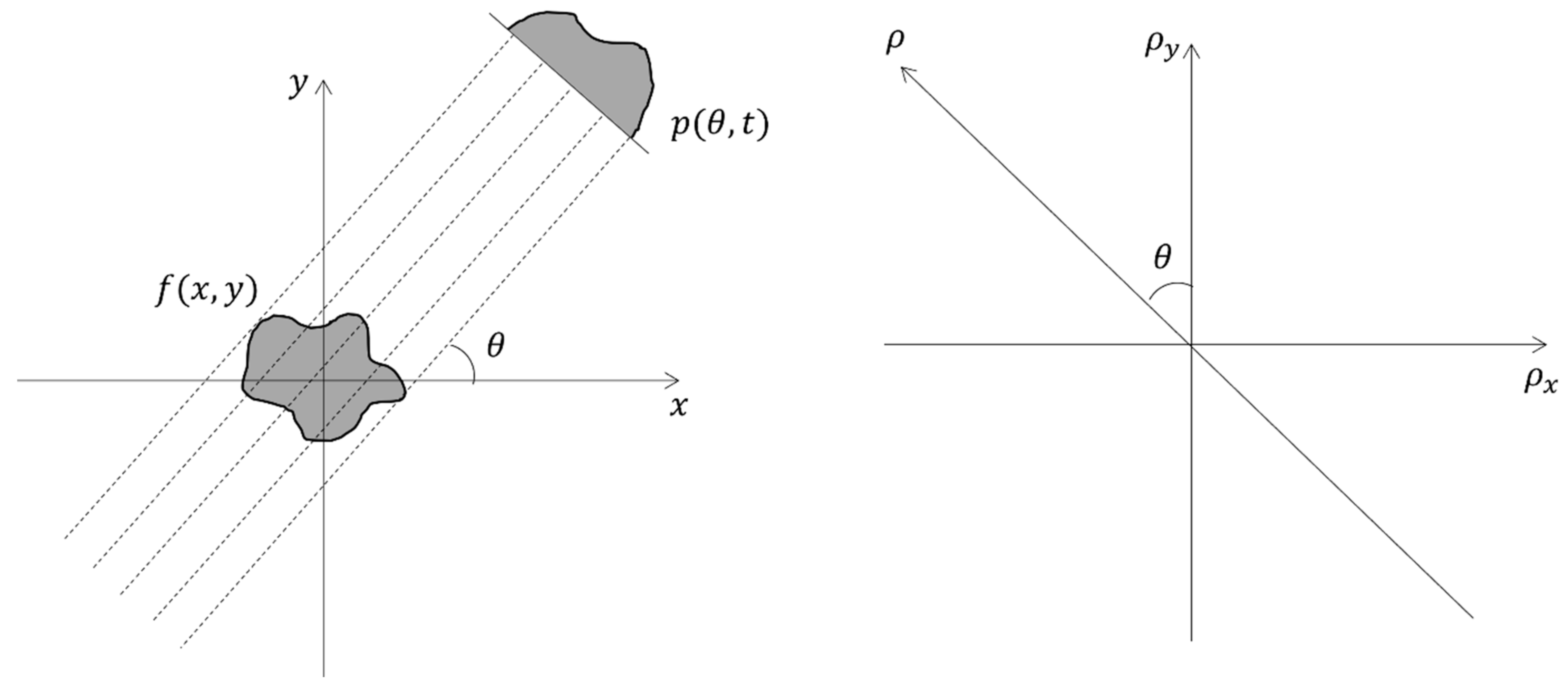
3.1. Preliminary
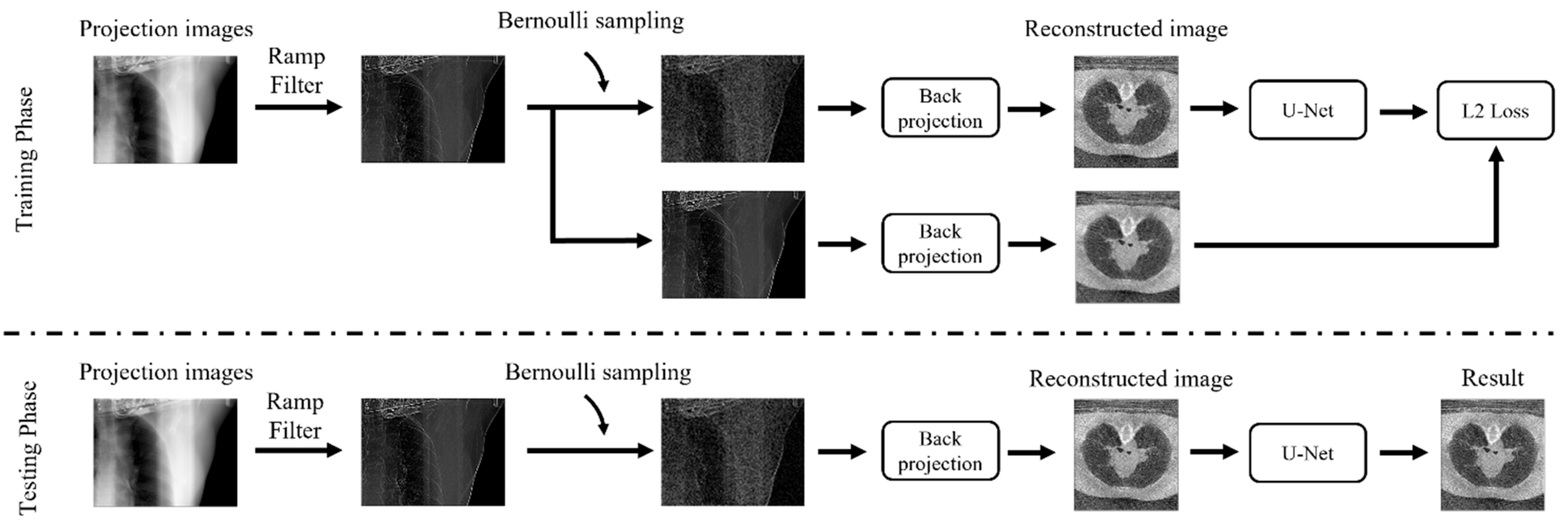
3.2. Dropped Projection Strategy
3.3. Training Scheme
3.4. Denoising Scheme
4. Experiments and Results
4.1. Evaluation Metrics
4.1.1. PSNR
4.1.2. SSIM
4.2. Implementation Details
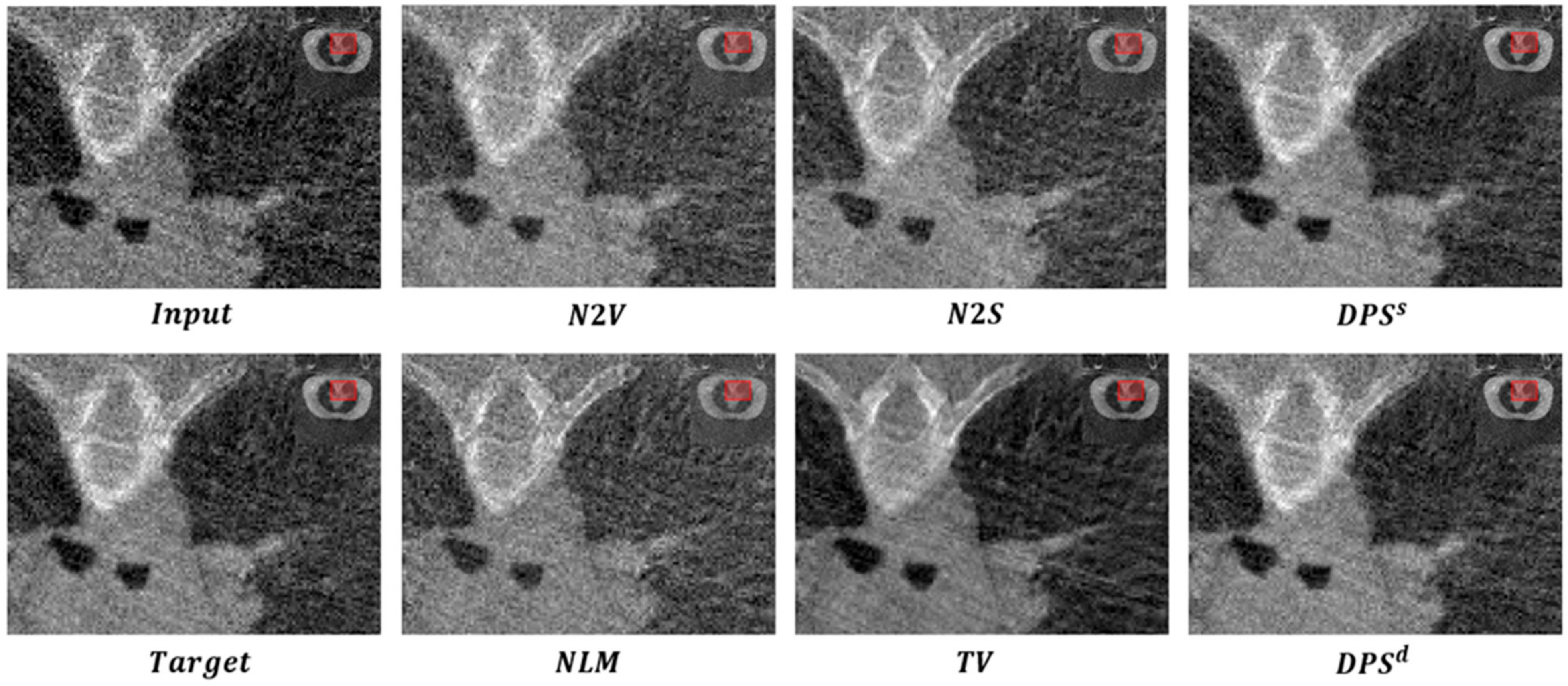
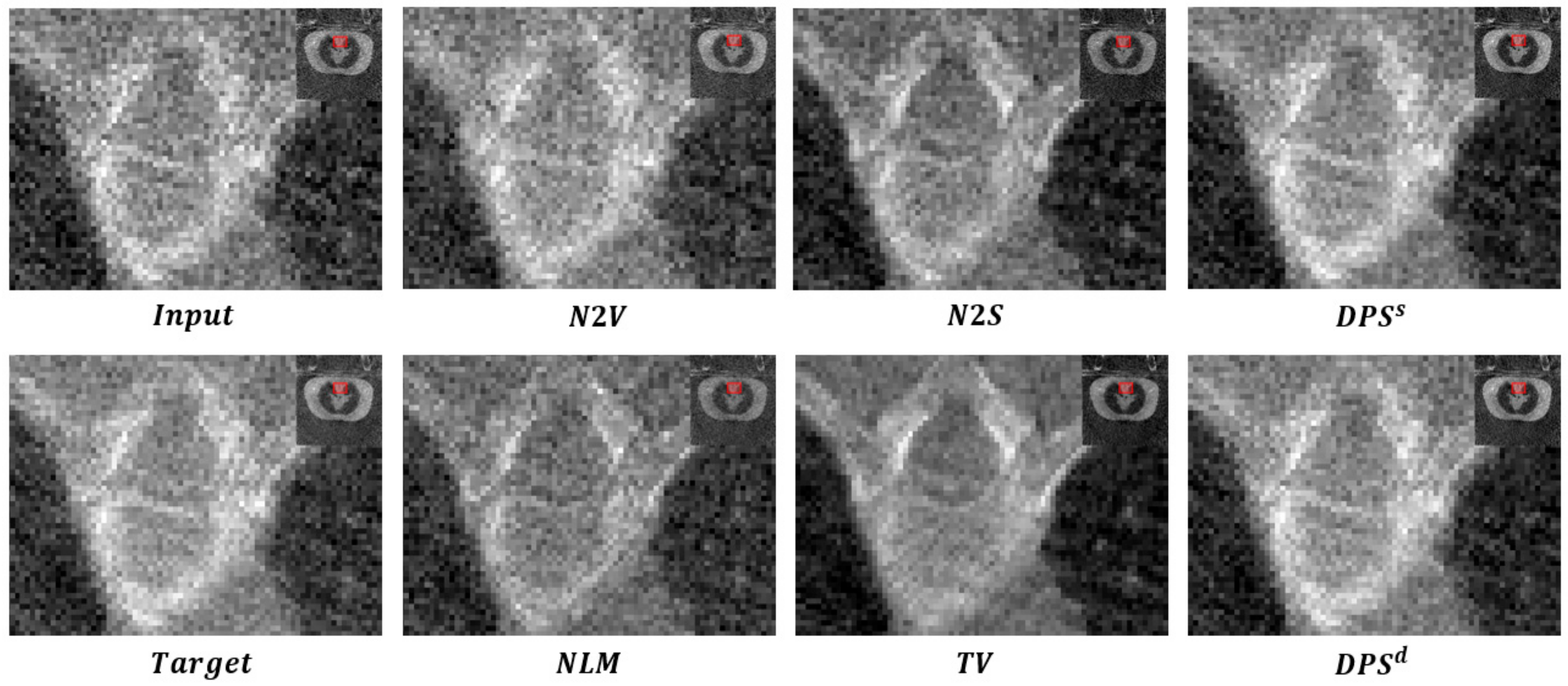
4.3. SPARE Challenge Dataset
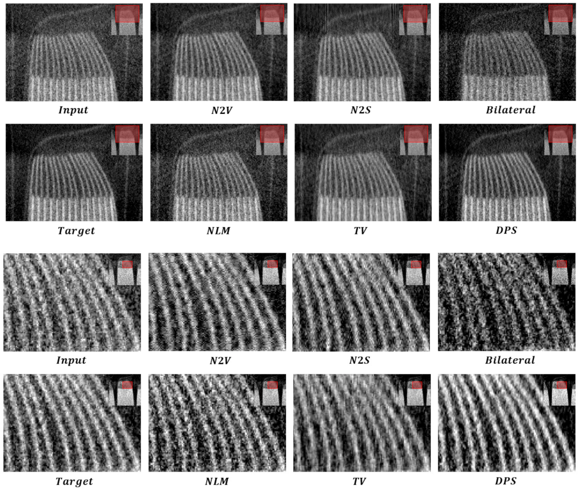
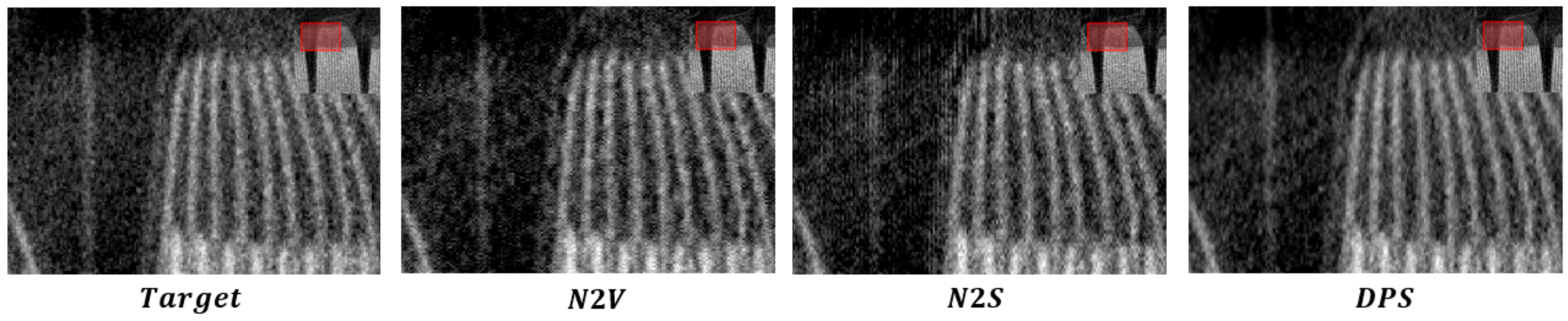
4.4. Lithium Polymer Battery Dataset
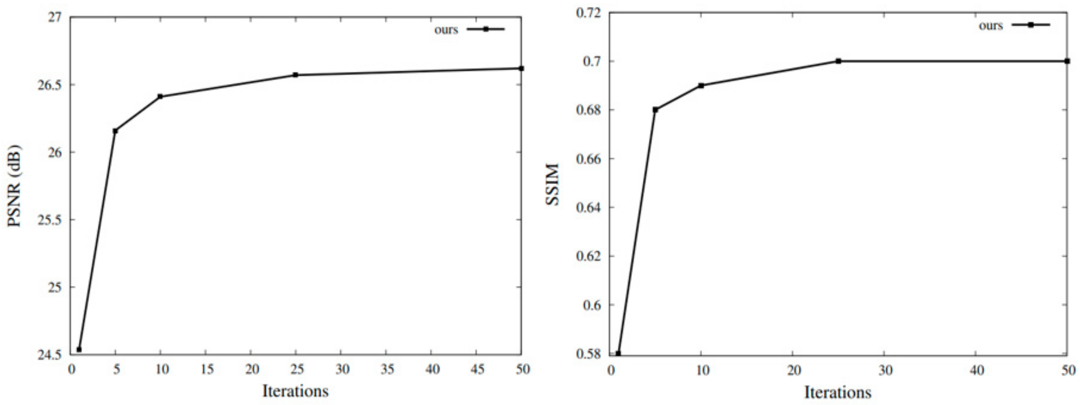
4.5. Performance for Repetition
5. Conclusions
Author Contributions
Funding
Institutional Review Board Statement
Informed Consent Statement
Conflicts of Interest
References
- Brenner, D.J.; Hall, E.J. Cancer risks from CT scans: Now we have data, what next? Radiology 2012, 265, 330–331. [Google Scholar] [CrossRef] [PubMed]
- Lee, S.; Lee, M.S.; Kang, M.G. Poisson–Gaussian noise analysis and estimation for low-dose X-ray images in the NSCT domain. Sensors 2018, 18, 1019. [Google Scholar] [CrossRef] [PubMed] [Green Version]
- Wang, J.; Lu, H.; Li, T.; Liang, Z. Sinogram noise reduction for low-dose CT by statistics-based nonlinear filters. In Proceedings of the Medical Imaging 2005, San Diego, CA, USA, 13–17 February 2005; pp. 2058–2066. [Google Scholar]
- Li, T.; Li, X.; Wang, J.; Wen, J.; Lu, H.; Hsieh, J.; Liang, Z. Nonlinear sinogram smoothing for low-dose X-ray CT. IEEE Trans. Nucl. Sci. 2004, 51, 2505–2513. [Google Scholar]
- Yu, L.; Manduca, A.; Trzasko, J.D.; Khaylova, N.; Kofler, J.M.; McCollough, C.M.; Fletcher, J.G. Sinogram smoothing with bilateral filtering for low-dose CT. In Proceedings of the Medical Imaging 2008, San Diego, CA, USA, 17–19 February 2008; pp. 768–775. [Google Scholar]
- La Rivière, P.J.; Bian, J.; Vargas, P.A. Penalized-likelihood sinogram restoration for computed tomography. IEEE Trans. Med. Imaging 2006, 25, 1022–1036. [Google Scholar] [CrossRef] [PubMed]
- Elbakri, I.A.; Fessler, J.A. Fessler. Statistical image reconstruction for polyenergetic X-ray computed tomography. IEEE Trans. Med. Imaging 2002, 21, 89–99. [Google Scholar] [CrossRef] [PubMed]
- Wang, J.; Li, T.; Xing, L. Iterative image reconstruction for CBCT using edge-preserving prior. Med. Phys. 2008, 36, 252–260. [Google Scholar] [CrossRef] [Green Version]
- Beister, M.; Kolditz, D.; Kalender, W.A. Iterative reconstruction methods in X-ray CT. Phys. Med. 2012, 28, 94–108. [Google Scholar] [CrossRef]
- Luo, X.; Yu, W.; Wang, C. An image reconstruction method based on total variation and wavelet tight frame for limited-angle CT. IEEE Access 2017, 6, 1461–1470. [Google Scholar] [CrossRef]
- Ertas, M.; Yildirim, I.; Kamasak, M.; Akan, A. An iterative tomosynthesis reconstruction using total variation combined with non-local means filtering. Biomed. Eng. Online 2014, 13, 65. [Google Scholar] [CrossRef] [Green Version]
- Kelm, Z.S.; Blezek, D.; Bartholmai, B.; Erickson, B.J. Optimizing non-local means for denoising low dose CT. In Proceedings of the 2009 IEEE International Symposium on Biomedical Imaging: From Nano to Macro, Boston, MA, USA, 28 June–1 July 2009; pp. 662–665. [Google Scholar]
- Xu, Q.; Yu, H.; Mou, X.; Zhang, L.; Hsieh, J.; Wang, G. Low-dose X-ray CT reconstruction via dictionary learning. IEEE Trans. Med. Imaging 2012, 31, 1682–1697. [Google Scholar]
- Li, Z.; Yu, L.; Trzasko, J.D.; Fletcher, J.G.; McCollough, C.H.; Manduca, A. Adaptive non-local means filtering based on local noise level for CT denoising. In Proceedings of the Medical Imaging 2012, San Diego, CA, USA, 5–7 February 2012; pp. 447–456. [Google Scholar]
- Kang, D.; Slomka, P.; Nakazato, R.; Woo, J.; Berman, D.S.; Kuo, C.-C.J.; Dey, D. Image denoising of low-radiation dose coronary CT angiography by an adaptive block-matching 3D algorithm. In Proceedings of the Medical Imaging 2013, Lake Buena Vista, FL, USA, 10–11 February 2013; pp. 671–676. [Google Scholar]
- Hasan, A.M.; Melli, A.; Wahid, K.A.; Babyn, P. Denoising low-dose CT images using multiframe blind source separation and block matching filter. IEEE Trans. Radiat. Plasma Med. Sci. 2018, 2, 279–287. [Google Scholar] [CrossRef]
- Chen, H.; Zhang, Y.; Kalra, M.K.; Lin, F.; Chen, Y.; Liao, P.; Zhou, J.; Wang, G. Low-dose CT with a residual encoder-decoder convolutional neural network. IEEE Trans. Med. Imaging 2017, 36, 2524–2535. [Google Scholar] [CrossRef] [PubMed]
- Kang, E.; Chang, W.; Yoo, J.; Ye, J.C. Deep convolutional framelet denosing for low-dose CT via wavelet residual network. IEEE Trans. Med. Imaging 2018, 37, 1358–1369. [Google Scholar] [CrossRef] [PubMed] [Green Version]
- Yang, Q.; Yan, P.; Zhang, Y.; Yu, H.; Shi, Y.; Mou, X.; Kalra, M.K.; Zhang, Y.; Sun, L.; Wang, G. Low-dose CT image denoising using a generative adversarial network with Wasserstein distance and perceptual loss. IEEE Trans. Med. Imaging 2018, 37, 1348–1357. [Google Scholar] [CrossRef]
- Tang, C.; Li, J.; Wang, L.; Li, Z.; Jiang, L.; Cai, A.; Zhang, W.; Liang, N.; Li, L.; Yan, B. Unpaired low-dose CT denoising network based on cycle-consistent generative adversarial network with prior image information. Comput. Math. Methods Med. 2019, 2019, 8639825. [Google Scholar] [CrossRef]
- Park, H.S.; Baek, J.; You, S.K.; Choi, J.K.; Seo, J.K. Unpaired image denoising using a generative adversarial network in X-ray CT. IEEE Access 2019, 7, 110414–110425. [Google Scholar] [CrossRef]
- Li, Z.; Zhou, S.; Huang, J.; Yu, L.; Jin, M. Investigation of low-dose CT image denoising using unpaired deep learning methods. IEEE Trans. Radiat. Plasma Med. Sci. 2020, 5, 224–234. [Google Scholar] [CrossRef]
- Lehtinen, J.; Munkberg, J.; Hasselgren, J.; Laine, S.; Karras, T.; Aittala, M.; Aila, T. Noise2noise: Learning image restoration without clean data. arXiv preprint 2018, arXiv:1803.04189. [Google Scholar]
- Krull, A.; Buchholz, T.O.; Jug, F. Noise2void-learning denoising from single noisy images. In Proceedings of the IEEE/CVF Conference on Computer Vision and Pattern Recognition, Long Beach, CA, USA, 15–20 June 2019; pp. 2129–2137. [Google Scholar]
- Batson, J.; Royer, L. Noise2self: Blind denoising by self-supervision. In Proceedings of the International Conference on Machine Learning, Long Beach, CA, USA, 10–15 June 2019; pp. 524–533. [Google Scholar]
- Quan, Y.; Chen, M.; Pang, T.; Ji, H. Self2self with dropout: Learning self-supervised denoising from single image. In Proceedings of the IEEE/CVF Conference on Computer Vision and Pattern Recognition, Online, 14–19 June 2020; pp. 1890–1898. [Google Scholar]
- Liang, K.; Zhang, L.; Xing, Y. Training a low-dose CT denoising network with only low-dose CT dataset: Comparison of DDLN and Noise2Void. In Proceedings of the Medical Imaging 2021, Online, 15–20 February 2021; p. 1159501. [Google Scholar]
- Unal, M.O.; Ertas, M.; Yildirim, I. Self-Supervised Training for Low-Dose Ct Reconstruction. In Proceedings of the 2021 IEEE 18th International Symposium on Biomedical Imaging (ISBI), Online, 13–16 April 2021; pp. 69–72. [Google Scholar]
- Tian, C.; Fei, L.; Zheng, W.; Xu, Y.; Zuo, W.; Lin, C.-W. Deep learning on image denoising: An overview. Neural Netw. 2020, 131, 251–275. [Google Scholar] [CrossRef]
- Radon, J. On the determination of functions from their integral values along certain manifolds. IEEE Trans. Med. Imaging 1986, 5, 170–176. [Google Scholar] [CrossRef]
- Turbell, H. Cone-Beam Reconstruction Using Filtered Backprojection. Ph.D. Thesis, Linköping University, Linköping, Sweden, 2001. [Google Scholar]
- Shieh, C.-C.; Gonzalez, Y.; Li, B.; Jia, X.; Rit, S.; Mory, C.; Riblett, M.; Hugo, G.; Zhang, Y.; Jiang, Z.; et al. SPARE: Sparse-view reconstruction challenge for 4D cone-beam CT from a 1-min scan. Med. Phys. 2019, 46, 3799–3811. [Google Scholar] [CrossRef] [PubMed]
- Wang, Z.; Bovik, A.C.; Sheikh, H.R.; Simoncelli, E.P. Image quality assessment: From error visibility to structural similarity. IEEE Trans. Image Process. 2004, 13, 600–612. [Google Scholar] [CrossRef] [PubMed] [Green Version]
- Isola, P.; Zhu, J.Y.; Zhou, T.; Efros, A.A. Image-to-image translation with conditional adversarial networks. In Proceedings of the IEEE Conference on Computer Vision and Pattern Recognition, Honolulu, HI, USA, 21–26 July 2017; pp. 1125–1134. [Google Scholar]
- Ronneberger, O.; Fischer, P.; Brox, T. U-net: Convolutional networks for biomedical image segmentation. In Proceedings of the International Conference on Medical Image Computing and Computer-Assisted Intervention, Munich, Germany, 5–9 October 2015; pp. 234–241. [Google Scholar]
- Kingma, D.P.; Ba, J. Adam: A method for stochastic optimization. arXiv preprint 2014, arXiv:1412.6980. [Google Scholar]


| Single Image Set Learning or Non-Learning Methods | Dataset-Based Deep Learning Method | |||||
|---|---|---|---|---|---|---|
| PSNR (dB) | 24.06 | 26.21 | 30.680 | 23.97 | 25.83 | 30.667 |
| SSIM | 0.55 | 0.65 | 0.787 | 0.56 | 0.67 | 0.786 |
| Single Image Set Learning or Non-Learning Methods | ||||||
|---|---|---|---|---|---|---|
| PSNR(dB) | 17.44 | 23.27 | 24.01 | 21.15 | 20.31 | 30.68 |
| SSIM | 0.21 | 0.70 | 0.64 | 0.37 | 0.24 | 0.79 |
Publisher’s Note: MDPI stays neutral with regard to jurisdictional claims in published maps and institutional affiliations. |
© 2022 by the authors. Licensee MDPI, Basel, Switzerland. This article is an open access article distributed under the terms and conditions of the Creative Commons Attribution (CC BY) license (https://creativecommons.org/licenses/by/4.0/).
Share and Cite
Han, Y.-J.; Yu, H.-J. Self-Supervised Noise Reduction in Low-Dose Cone Beam Computed Tomography (CBCT) Using the Randomly Dropped Projection Strategy. Appl. Sci. 2022, 12, 1714. https://doi.org/10.3390/app12031714
Han Y-J, Yu H-J. Self-Supervised Noise Reduction in Low-Dose Cone Beam Computed Tomography (CBCT) Using the Randomly Dropped Projection Strategy. Applied Sciences. 2022; 12(3):1714. https://doi.org/10.3390/app12031714
Chicago/Turabian StyleHan, Young-Joo, and Ha-Jin Yu. 2022. "Self-Supervised Noise Reduction in Low-Dose Cone Beam Computed Tomography (CBCT) Using the Randomly Dropped Projection Strategy" Applied Sciences 12, no. 3: 1714. https://doi.org/10.3390/app12031714