Feature Transformation Framework for Enhancing Compactness and Separability of Data Points in Feature Space for Small Datasets

Abstract

Compactness and separability of data points are two important properties that contribute to the accuracy of machine learning tasks such as classification and clustering. We propose a framework that enhances the goodness criteria of the two properties by transforming the data points to a subspace in the same feature space, where data points of the same class are most similar to each other. Most related research about feature engineering in the input data points space relies on manually specified transformation functions. In contrast, our work utilizes a fully automated pipeline, in which the transformation function is learnt via an autoencoder for extraction of latent representation and multi-layer perceptron (MLP) regressors for the feature mapping. We tested our framework on both standard small datasets and benchmark-simulated small datasets by taking small fractions of their samples for training. Our framework consistently produced the best results in all semi-supervised clustering experiments based on K-means and different seeding techniques, with regards to clustering metrics and execution time. In addition, it enhances the performance of linear support vector machine (LSVM) and artificial neural network (ANN) classifier, when embedded as a preprocessing step before applying the classifiers.

1. Introduction

One of the fundamental concepts in machine learning is the embedding of data points in an appropriate feature space [1]. The choice of the feature space should be driven by enhancing the topological properties of data clusters, ultimately leading to better performance in pattern recognition tasks such as classification [2,3,4], clustering [5,6,7], information retrieval [8,9,10,11], and regression [12,13]. Data points and latent features are two spaces where feature engineering approaches operate.

One approach is projecting the data descriptors to an alternative feature space via a hard-coded mathematical function. The evident example of this approach is the use of kernel functions in SVM classifiers, aiming to improve the separability property to allow efficient localization of the hyperplane [14]. Another example is the latent representation yielded on the hidden layers of ANNs [15,16]. The goal is to increase the compactness of the class samples by abstracting the input data from its specifics and details. Clearly there is a difference between SVMs and ANNs in the intermediate goal; one opts for increasing separability while the other increases compactness. In addition, in the former technique, the mapping is hand-engineered kernels, whereas in the latter the mapping function is learned.

On another front, feature transformations retaining the original data space have been limited to feature selection, normalization, and scaling [17]. Conceptually, non-parametric learning approaches such as KNN [18] also belong to this paradigm of feature transformation and can be regarded as a projection of test samples into a subspace of training samples. When the model is presented with unseen data, it uses a distance function to map the data to the most similar pre-seen example. In essence, it is a classification approach with a hypothetical embedded feature transformation step based on a distance mapping function. Limitations of KNN have been thoroughly discussed in the literature [19,20,21,22]. One of its drawbacks is the reliance of the mapping function on a linear distance measure [20] (e.g., Manhattan, Euclidean, Minkowski, and weighted Euclidean distance) between corresponding individual features. However, it neglects the interrelation between features comprising the data samples and their collaborative effect, thus limiting the ability of the distance function in expressing the similarity/dissimilarity of the samples [22]. In addition, the KNN method does not promote properties of compactness and separability of data embeddings in the feature space.

Additionally, oversampling approaches operate both spaces [17,23]. Oversampling creates synthetic examples by relocating feature vectors of given examples along the line segments joining the $k$ nearest neighbor examples of the same class. Although this approach shows improvement in the accuracy of classification tasks in case of imbalanced and small datasets, it does not improve the compactness and separability of data points. It could happen that a minority class sample could have a majority class sample as its neighbor, which will create false positive samples.

State-of-the-art deep learning algorithms have achieved near-human-level accuracy in applications such as computer vision [24,25,26,27,28]. Nevertheless, one challenge remains for these algorithms when faced with inadequate amounts in acquiring adequate amounts of labeled data [29]. Otherwise, these models are subject to overfitting [30] due to the large number of parameters to learn in complex networks which reduce the network’s ability to generalize and cause the network to memorize examples. Also, labeling is widely regarded as a manual labor-intensive and resource-consuming process. In other cases, there are great difficulties in the initial acquisition process of the data samples, a problem that is well-known in the field of bioinformatics [31]. All these factors result in the occurrence of small-sized datasets in either supervised or semi-supervised settings, thus limiting the generalization ability of the end classifier [32]. This challenge is exaggerated in the case of the existence of high intra-class variability [33,34], which leads to classes of low density in the feature space. In fact, these challenging factors impact clustering algorithms as well [35]. Concurrently, they have a jarring effect on the clusters, creating disjoint subdivisions and hindering the discovery of the class structure in its entirety in space.

In our work, the main contribution is proposing a model architecture which fully automates the learning of the transformation function that operates on unseen samples so that they resemble approximations of samples encountered in the training set. There are two aspects evident in our framework. First, we preserve the same feature space as the original data points. Second, we relocate input samples in a subspace while improving the goodness criteria of separability and compactness [36,37,38,39]. To the best of our knowledge, this is the first time these aspects have been combined to carry out the task of selecting the feature vector embedding space.

To this end, we train two main network models that, combined, comprise the transformation function. We train an autoencoder for feature extraction and reconstruction of the training samples. We create Cartesian product pairs of the training samples resulting in a set of ordered pairs and extract their embeddings from the encoder of the trained autoencoder. Then, a bridging regression network learns to map the embeddings of the first element in each ordered pair (as input variables to the regression network) to the embeddings of the second element in the pair (as target variables). We use the encoder of the autoencoder, the bridging network, and the decoder from the autoencoder to transform the training and test samples of each class to very similar (template-like) samples of the same class resulting in a reduction in intra-class variance and an increase in the inter-class variance. This helps to enhance the accuracy over the transformed test set of an off-the-shelf classifier trained on the training samples augmented with the transformed training samples.

Data augmentation [17] is an effective technique to handle overfitting in the case of small datasets and enhance generalization of the machine learning model, particularly ANNs, by increasing both amount and diversity of data samples. The significance of our work is highlighted in the case of small datasets ($\left|n\right|$) with high variability. We fully exploit the samples available in the datasets by a pairing mechanism where we pair each example with all other examples of the same class and we study the samples’ inter-relations $\left|n^2\right|$, thus incrementing the learning data pool. In addition, we augment the dataset with reconstructions of latent features of the samples after being subjected to a regression step.

Another contribution to this work is the applicability of our proposed model in a semi-supervised clustering setting where a few labeled data samples are utilized to learn clustering of the plentiful unlabeled data in a partially labeled dataset [40,41]. We use the labeled data samples to train our model to learn the transformation function, then we transform the unlabeled data using our trained model. We feed the transformed examples to a clustering technique. We show that not only is the clustering time of the transformed data points significantly reduced compared to using the same clustering techniques on the untransformed data points, but also all clustering metrics used to measure the performance of the clustering techniques notably improve.

Several efforts have been proposed in the field of feature engineering in general and in the settings where there is a focus on improving compactness and separability. Feature engineering is a preprocessing task to improve the prediction performance of a machine learning model on a dataset by applying a transformation function on its feature space. Many feature engineering techniques [42] yielding feature vectors in the same input data space are limited to scaling and normalization or simply applying hand-crafted arithmetic or aggregation functions to the features to construct more suitable features benefitting the machine learning model’s performance. One problem of feature engineering is finding a particularly good transformation for a given set of features given a set of transformation functions. In [3], instead of enumerating and trying all transformation functions and their combinations by training and testing models, which is computationally impractical, the authors automate the decision-making process of recommending the transformation functions applied to the features. In our work, our aim is to learn the transformation function, instead of using hand-crafted transformation functions, and using our learnt parameters to relocate the feature space of the data samples.

Intra-class compactness and inter-class separability are commonly studied in the field of machine learning. The two characteristics are crucial measures of how effectively a model produces discriminant features. Approaches vary in tackling the problem of improving compactness and separability of features. In [39], the authors propose a feature optimizer that calculates a center for each class by averaging samples in a mini-batch and optimizes the calculated centers at each iteration by minimizing a feature optimization loss that consists of two distances, the distance of samples in the mini-batch to its correct center, and the other is to its nearest wrong center. Another approach that extends the loss function of a model is proposed by Pilarczyk et al. [36]. They use intra-class variance loss as a regularization term for training deep neural network (DNN) classifiers. This approach is different from the previous approach as the centroids of classes that contribute to calculating the intra-class variance loss are learned through an additional Hadamard layer attached to the convolutional neural network (CNN) architecture where its parameters represent the class centers. Luo et al. [37] proposed a Gaussian-based Softmax function that can be easily implemented and can replace the Softmax function in CNNs. The proposed function improves intra-class compactness and inter-class separability that improves classification on several multi-label classification datasets. Liu et al. [38] proposed to employ a margin constraint in the original Softmax function which explicitly encourages the learning of more discriminative features.

All the aforementioned approaches show the importance of enhancing the discriminant nature of learned features which consequently improves the performance of underlying models. However, a common limitation of these approaches is that they extend or change the used loss function in DNN architectures limiting the choice of classifiers to DNN classifiers. This conclusion encourages us to tackle the problem using a different approach. Our approach uses a combination of supervised and generative models that create a framework for transforming the learned features into an enhanced feature subspace promoting the compactness and separability of classes. Our proposed model is a pluggable model before any classifier type model not limited by a particular type of classifiers, as in other approaches.

We also investigate the intra-cluster compactness and inter-cluster separability in the field of unsupervised and semi-supervised learning to enhance clustering performance. Most hard clustering techniques such as basic K-means [43] and clustering algorithms are based on K-means [44,45]. These types of clustering algorithm work by only minimizing the within-cluster distance while neglecting the between-cluster distance. Huang et al. [46] proposed a series of extension to the K-means-based clustering algorithms where they utilize the idea of a global centroid and maximizing the distance between clusters’ centroids (increasing the between-cluster separation) while still minimizing the distances between data points and the centroids of the clusters (improving the within-cluster compactness). Soft-clustering algorithms that utilize the intra-cluster as well as the inter-cluster distances have also emerged, such as enhanced soft subspace clustering (ESSC) [47] and supervised enhanced soft subspace clustering (SESSC) [48]. SESSC is based on ESSC which considers both the within-cluster compactness and between-cluster separation. In addition, SESSC takes advantage of the label information in a semi-supervised setting. Therefore, SESSC can be used as a standalone classifier or integrated into a fuzzy classifier to further improve its performance.

The remainder of the paper is organized into three sections. Section 2 elaborates on our proposed method in three subsections corresponding to three modules of the proposed framework. Section 3 illustrates our conducted experiments and the evaluation of the proposed framework in two settings, a semi-supervised clustering setting, and a supervised setting. Finally, Section 4 concludes the paper.

2. Method

Given a dataset $D=\left\{D^{Tr}, D^{Ts}\right\}$ split into two subsets, there are a training set $D^{Tr}$ and a testing set $D^{Ts}$ with ${\mathcal{L}}_{Tr}={\left\{{\ell }_i\right\}}_{i=1}^N$ and ${\mathcal{L}}_{Ts}={\left\{{\ell }_i\right\}}_{i=1}^M$ where $N$ and $M$ are $\left|D^{Tr}\right|$ and $\left|D^{Ts}\right|$, respectively. Typically, the given dataset is a small dataset or a dataset with very small number of labeled examples compared to the number of unlabeled examples $N\ll M$. The aim for our model is to learn a transformation function $f\left(X^k\right)=Y^k | Y^k\cong {\mu }^k, k=0\dots K-1$ where $K$ is the number of classes in the dataset. The function maps each sample ($x_i^k\in X^k$) of the same class to a $y_i^k$, where $y_i^k$ approximates ${\mu }^k$ centroid (mean sample) of the same class.

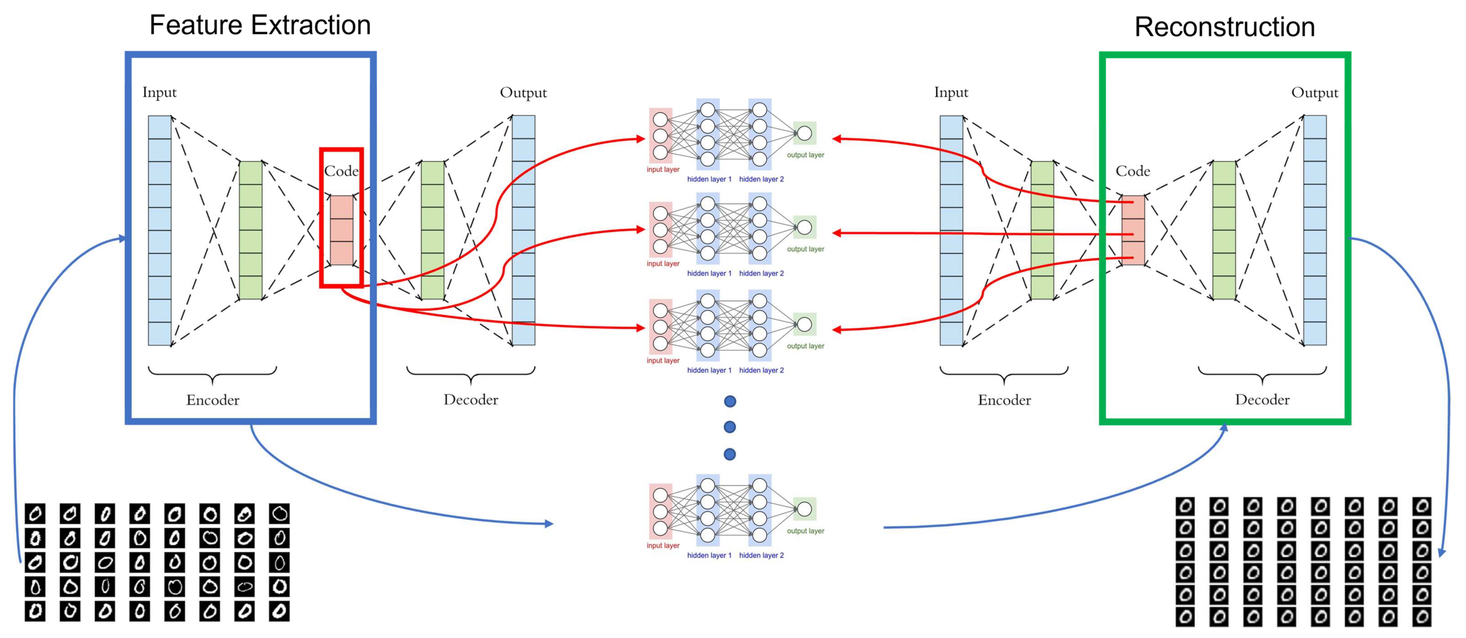
As illustrated in Figure 1, our proposed framework consists of three main modules: feature extraction, feature mapping, and reconstruction. For feature extraction, we train an autoencoder [49] $AE$, which is a generative model that reconstructs the available training samples in the dataset $X^k$, through learning their latent representation. In the feature mapping module, we first pair the training samples of each class with all other samples of the same class. Second, we use the trained autoencoder to extract the features of the pairs. Then, we train a mapping network that consists of a set of multilayer perceptron (MLP) regressors $\mathrm{B}=\left\{ML{P}_1, ML{P}_2, \dots , ML{P}_{N_f}\right\}$, where $N_f$ is the number of latent features in the embedding layer $Z$ of the autoencoder $AE$. Each MLP regressor in the network learns to output $z_i^s\in Z, s=1, 2, \dots , N_f$. Finally, we take the mapped latent features $\widehat{Z}$ from the feature mapping network $\mathsf{{\rm B}}$ and feed it into the decoder of the trained autoencoder to reconstruct the mapped samples $Y^k$.

After training the whole framework, we use it to map the test set examples to a more compact space for intra-class samples and separable for inter-class samples. Evaluating a classifier on the transformed samples gives better accuracy and loss than evaluating the same classifier on the untransformed examples. In the next three subsections, we explain the details of the three modules composing our framework.

2.1. Feature Extraction Using Autoencoders

Autoencoders are neural networks that are unsupervised (they can be thought of as self-supervised) learning models. Autoencoders were first introduced in [50] as neural networks that learn the compressed internal representation of some input while reconstructing the same input. An autoencoder tries to learn a function $g_{W, b}\left(x\right)=\widehat{x}$ by minimizing the reconstruction error of the input so that $\widehat{x}$ is as similar as possible to $x$. The autoencoder achieves this by encoding the input into the feature space using an encoder subnetwork, then decodes it back using a decoder subnetwork [49,51]. The learned representation (latent features) can be extracted and used in different machine learning tasks [52,53,54,55]. Following the same notion, we use autoencoders in our framework to extract features $Z$ of samples $X^k$ that are used as input in the next module of the framework for training the bridging network of MLP regressors.

The mathematics of an autoencoder can be formulated as defined in [56] as follows:

$$E:X\to Z,$$

(1)

$$D:Z\to \widehat{X},$$

(2)

Such that (1) and (2) satisfy:

$$\arg min{ }_{E, D}\mathbb{E}\left[\Delta \left(X, D\circ E\left(X\right)\right)\right],$$

(3)

where $\mathbb{E}$ is the expected value of the reconstruction error function $\Delta$ over the distribution of $X$. $E$ is the encoder function that maps the original input $X$ to a latent representation $Z$ at the bottleneck of the autoencoder. The decoder function $D$ does the opposite by mapping the latent features $Z$ at the bottleneck to the output of the decoder network approximating the original input $X$. Training the encoder and the decoder networks involves optimizing the networks’ parameters $\left(W, b\right)$ through backpropagating the reconstruction error between the decoder’s output and the original input.

In our framework, we train a deep autoencoder network on the training set $D^{Tr}$, such that the autoencoder learns a latent representation $Z$ for all samples in the dataset while minimizing the mean-squared error (MSE) (as the error function $\Delta$) of the decoder reconstructions.

2.2. Feature Mapping Network

In this module, we aim to train a network to learn a transformation function that could later be used to map the testing set to a feature space with improved properties of separability and compactness. Our approach is to learn a regression function that transforms the distribution of the embeddings of each class to a more compact distribution. As we shortly show, regressors with high bias and low variance tend to output a value close to the average of the target. Following this observation, we want to force the regression model even more to learn a value close to the average of each feature embedding.

Bias-variance tradeoff is a widely studied problem in the field of machine learning [57,58]. The dilemma was first formally introduced in [59], and it refers to a model property where the estimation error of the model can be decomposed into two terms, known as bias and variance, thus, either bias or variance can affect the performance of a model. The bias error is the difference between the expected (average) prediction of our model and the target correct value which results from oversimplifying the estimated function and missing the regularities in the training data. The variance error is the difference between the average prediction of our model for a given data point which results from the sensitivity of the model to irregularities in the training data.

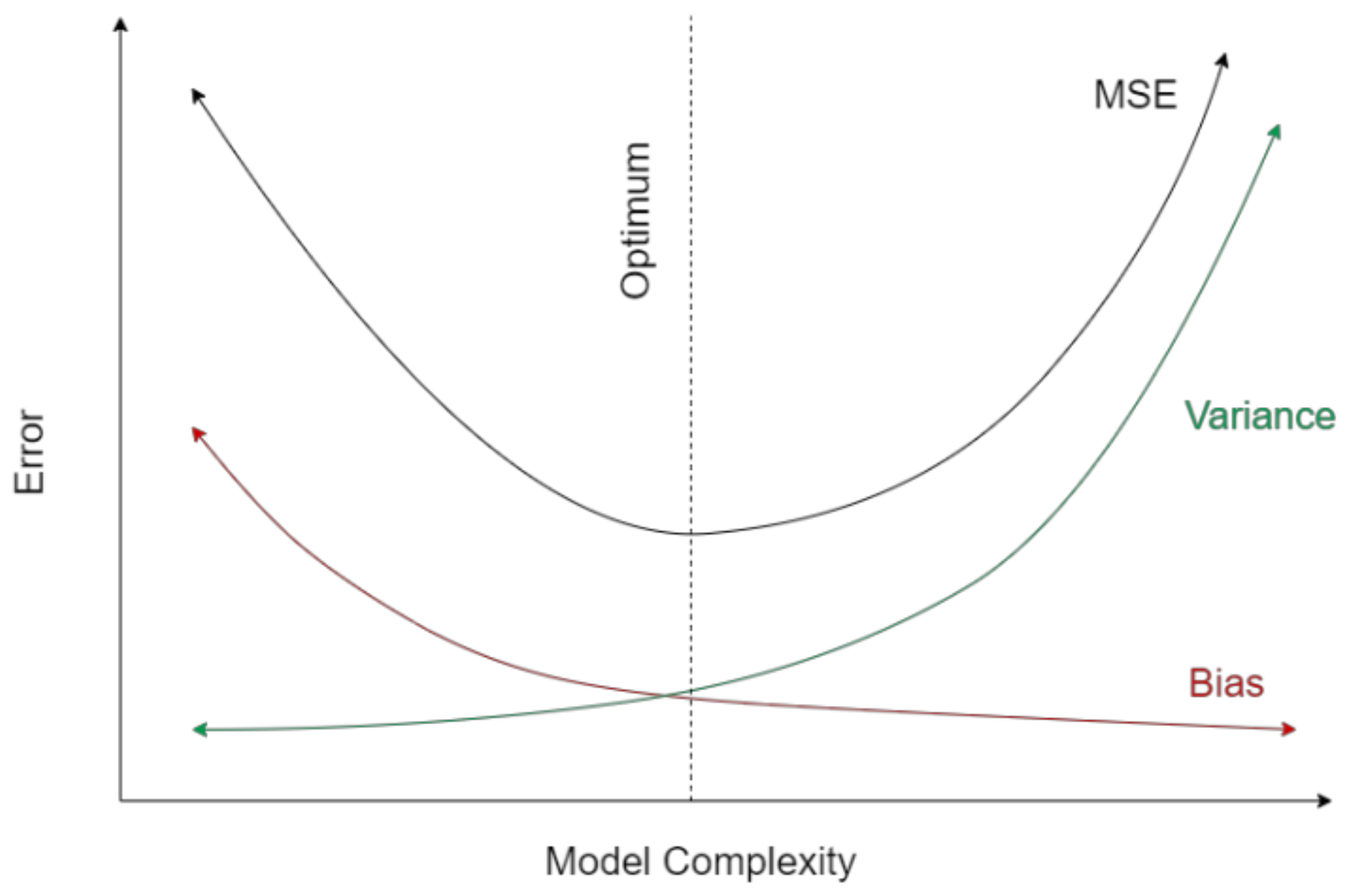
As illustrated in Figure 2, there is often a tradeoff between the contribution of bias and variance to the estimation error as conflict arises from trying to simultaneously minimize the two error terms. The variance error can be reduced through smoothing the signal which will in effect introduce a high bias as the model will be oversmoothed and will miss the specifics of the underlying data points resulting in an underfitting scenario where both the training and test errors are high. On the other hand, the high bias can be reduced by increasing the complexity (number of fitting parameters) of the model, but then the variance of the model will increase as the model will have more capacity to fit the noise and irregularities of the underlying training data points and not generalizing to the target signal. This scenario is referred to as overfitting, giving a low training error while degrading the predictive performance on the test data.

As we observe, the MLP regressor models for the bridging network learn to predict the average value of the target feature values for the same class. The intuition behind that observation is that the model is not complex enough to fit the underlying data (underfitting to data points), which means the model has too much bias. According to the bias-variance tradeoff, the high bias model will have a low variance to reduce the whole mean-squared error ($MSE$), which decomposes into the two terms of $Bias$ and $Variance$:

$$MSE=Bia{s}^2+Variance$$

(4)

In the book Doing Bayesian data analysis [60], the author stated that the mean of a distribution is the value that minimizes the expected squared deviation. As can be mathematically proven (see Appendix A), the mean-squared error has a lower bound value as the variance of $Y$ (the target output) when $\widehat{Y}$ (the predicted output) equals the average of $Y$. Therefore, the model will predict values closer to the average, trying to reach the lower bound of the $MSE$.

We also found that if we train the regressor with different outputs for the same set of corresponding inputs, the regressor will minimize its error by outputting a value close to the average of the presented target values. A plausible explanation for this behavior is that having different target values for the same input features resembles adding noise to the output. Adding noise to the input or the output (less common) is a well-known regularization method to aid generalization (lowering the variance) and avoid overfitting [61,62,63]. According to the bias-variance tradeoff theory, reducing the variance error will, in effect, give a high bias model as the model’s error decomposes into bias and variance errors. Therefore, adding variant targets for the same input encourages the network’s output to be a smooth function of the input.

To feed the regressors with different target outputs for the same latent representation, we pair the features of each example with $m$ examples of the same class. We experimented with different values for $m$, but we found that pairing each example with all other examples of the same class ($m=\left|D_k\right|$) gives better results.

The pairing algorithm can be described as getting the Cartesian Product for each set of samples $D_k$ belonging to the same class with itself. Identical ordered pairs are excluded.

$$T_{CP}=D_k\times D_k=\left\{\left(a, b\right) | a\in D_k and b\in \left\{D_k-\left\{a\right\}\right\}\right\} \forall k\in K$$

(5)

As described in Algorithm 1, we do the Cartesian product of each class $k$ set of samples by pairing each sample with all other samples of the same class $k$, such that if we have $m$ examples in a class, we end up having $m\times \left(m-1\right)$ samples per class in the Cartesian product set $T_{CP}$. We form two sets $T_1$ and $T_2$ from the ordered pairs of the Cartesian product set $T_{CP}$ such that $T_1=\left\{a_i\right\}, i=0, 1,\dots , m$ and $T_2=\left\{b_j\right\}, j=0, 1,\dots , m$ and $i\ne j$, i.e., we form two sets, $T_1$ for the first elements and $T_2$ for the second elements of the ordered pairs. The pairing algorithm is applied to the training set $D^{Tr}$ where we group the training samples by labels ${\mathcal{L}}_{Tr}$, and results in two sets $T{r}_1 \mathrm{and} T{r}_2$ (ground truth training set for the feature mapping network) with repeated examples in each, where $\left|T{r}_1\right|=\left|T{r}_2\right|=m\times \left(m-1\right)\times K$.

Algorithm 1. The Pairing Algorithm.
Require:	$D^{Tr}$, ${\mathcal{L}}_{Tr}$, $K$
1	$Group D^{Tr} by {\mathcal{L}}_{Tr}$
2	$T{r}_1\leftarrow \left[ \right], T{r}_2\leftarrow \left[ \right], {\mathcal{L}}_{Tr}{}_1\leftarrow \left[ \right], {\mathcal{L}}_{Tr}{}_2\leftarrow \left[ \right]$
3	$st=0$
4	for $k\leftarrow 0 to K-1$ do
5	$m\leftarrow getClassLength\left(k\right)$
6	for $i\leftarrow 0 to m$ do
7	for $j\leftarrow 0 to m, j\ne i$ do
8	$append D^{Tr}{}_{\left[st+i\right]} to T{r}_1$
9	$append D^{Tr}{}_{\left[st+j\right]} to T{r}_2$
10	$append {\mathcal{L}}_{Tr}{}_{\left[st+i\right]} to {\mathcal{L}}_{Tr}{}_1$
11	$append {\mathcal{L}}_{Tr}{}_{\left[st+j\right]} to {\mathcal{L}}_{Tr}{}_2$
12	end
13	$st=st+m$
14	end
15	end

After we have our two training sets ($T{r}_1, T{r}_2$) from the pairing algorithm, we extract the features $Z_1$ and $Z_2$ (ground truth latent features) for the two sets $T{r}_1$ and $T{r}_2$ using our trained autoencoder $AE$ from the previous module. For the mapping network, we train a set of MLP regressors $\left\{ML{P}_1, ML{P}_2, \dots , ML{P}_{N_f}\right\}$ where $N_f$ is the number of embedded features $\left|Z_2\right|$, such that each MLP regressor corresponds to one latent feature $z_{2, i}^s$ of the $N_f$ features in $Z_2$, and we use $Z_{1, i}$ as the same input for all MLP regressors. We can either train the $N_f$ MLP regressors serially or in parallel as they correspond to independent outputs, so we choose to train them in parallel to speed up the training process.

2.3. Mapped Features Reconstruction

In the third module of our framework, we use the decoder of the trained autoencoder $AE$ to reconstruct the latent representations $\widehat{Z}$ obtained from the regressors, in the feature mapping network module, back to the input space $Y^k$, where $y_i^k$ approximates ${\mu }^k$ centroid (mean sample) of the same class.

A summary of the transformation pipeline is shown in Algorithm 2. Given a training set $D^{Tr}$ and a test set $D^{Ts}$, we first extract the features $Z_{tr}$ of $D^{Tr}$ from the trained autoencoder $AE$ and map $Z_{tr}$, using the trained regressors in the feature mapping network $B$, to $\widehat{Z_{tr}}$, then, we use the decoder of $AE$ to reconstruct $\widehat{Z_{tr}}$ to the input space yielding $\widehat{D^{Tr}}$. We do the same for $D^{Ts}$ resulting in the transformed test set $\widehat{D^{Ts}}$.

Our proposed framework can be embedded as a preprocessing step in semi-supervised and supervised settings. In the semi-supervised setting, we use the limited training (labeled) set $D^{Tr}$ to train our framework and transform the test (unlabeled) set $D^{Ts}$ and cluster the transformed unlabeled set $\widehat{D^{Ts}}$ using a clustering algorithm. In the supervised setting, we use an off-the-shelf classifier in the following setting: the plain training set $D^{Tr}$ augmented with the transformed training set $\widehat{D^{Tr}}$ using our framework as shown in Algorithm 2. The augmentation of the mapped training samples increases the size of the learning data pool which is beneficial in the case of small size datasets where the lack of training samples increases the chance of overfitting. Our augmentation resembles SMOTE augmentation in that we both operate in the feature space to generate the augmented samples. However, our augmentation is different in that we do not interpolate new data samples among a number of neighboring samples, conversely, we transform the available data samples to a group of similar data samples approximating the mean sample of the target class. Also, SMOTE increases the density of samples of the same class within the same boundaries of data clusters without relocation of clusters which does not provide any improvement in the separability and compactness characteristics.

Algorithm 2. The Transformation Pipeline.
Require:	$D^{Tr}, D^{Ts}$
1	$Z_{tr}\leftarrow Extract features of D^{Tr} from the trained autoencoder AE$
2	$\widehat{Z_{tr}}\leftarrow Predict features using the trained MLP regressors and Z_{tr} as input$
3	$\widehat{D^{Tr}}\leftarrow Reconstruct the predicted features \widehat{Z_{tr}} using the decoder of AE$
4	$Repeat for D^{Ts}$

3. Evaluation

To evaluate our proposed model, we tested our model in two different machine learning tasks: semi-supervised clustering and classification. We conducted experiments on five different datasets, and we calculated various clustering metrics for the semi-supervised clustering setting that show the model’s ability to achieve its goal of improving compactness and separability among targets. Also, we showed that the model enhances an off-the-shelf classifier’s accuracy indicating the classifier is able to achieve better decision boundaries on the target classes.

3.1. Datasets

We evaluated our proposed model on five different datasets. We used the three standard benchmark datasets: MNIST [64], Fashion-MNIST [65], USPS [66], and we further evaluated our model on two already small datasets: the three-target MSTAR dataset [67] which is widely used in automatic target recognition (ATR) of synthetic aperture radars (SAR) images, and the Breast Cancer Wisconsin (WDBC) dataset from the UCI repository [68]. For the benchmark datasets (MNIST, Fashion-MNIST, and USPS), we used a very small subset of the training examples to simulate a limited training data problem, and we appended the remaining training images to the test set.

Both MNIST and Fashion-MNIST datasets contain 60,000 training and 10,000 test samples, while the three-target MSTAR and WDBC datasets contain only 698 and 569 training samples, respectively, which are significantly less than those in the MNIST and Fashion-MNIST datasets. Therefore, we chose at random a ratio of 1% per class of the training images and appended the remaining images to the test set. We ended up with 596 training and 69,404 test images for the MNIST dataset, and 600 training and 69,400 test images for the Fashion-MNIST dataset. For the USPS dataset, which consists of 7291 training and 2007 test images, we selected 10% of the training images per class making a total of 725 training and 8573 test images. The samples of the WDBC dataset were split into 70% (398) training and 30% (171) testing samples. A summary of the number of training and testing samples, number of classes, and input sizes is listed in

Table 1. The number of training and testing samples, number of classes, and input sizes for each dataset.

Dataset	MNIST	Fashion-MNIST	USPS	MSTAR	WDBC
No. of Training Samples	596	600	725	698	398
No. of Testing Samples	69,404	69,400	8573	587	171
No. of Classes	10	10	10	3	2
Input Size	28 $\times$ 28	28 $\times$ 28	16 $\times$ 16	128 $\times$ 128	30

.

3.2. Experimental Setup

We used an autoencoder architecture for feature extraction. The autoencoder architecture vary from dataset to another. A summary of the autoencoder architecture, batch size and number of epochs used for each dataset is presented in

Table 2. Autoencoder architecture, batch sizes and number of epochs for each dataset.

Dataset	MNIST	Fashion-MNIST	USPS	MSTAR	WDBC
Flattened Input Size	784	784	256	16,384	30
AE Architecture	512-256-512	512-256-512	512-128-512	256-64-256	32-16-32
Batch Size	50	50	50	50	10
No. of Epochs	1200	1200	600	100	200

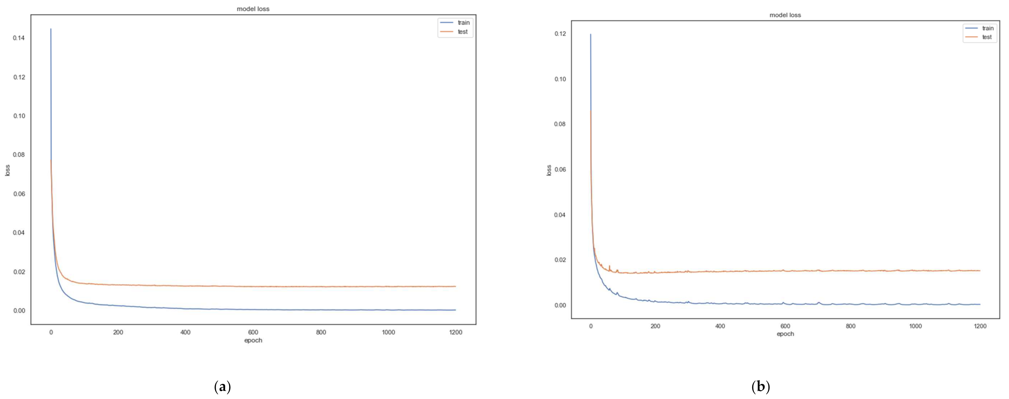
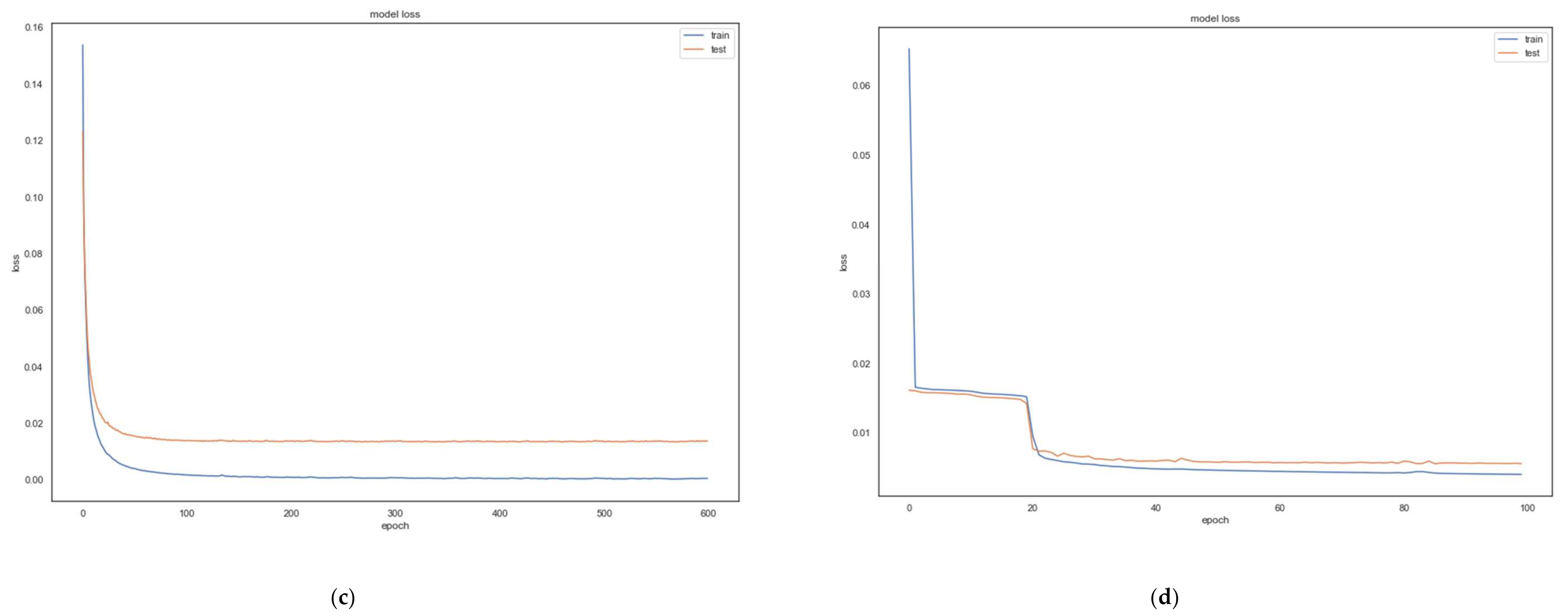
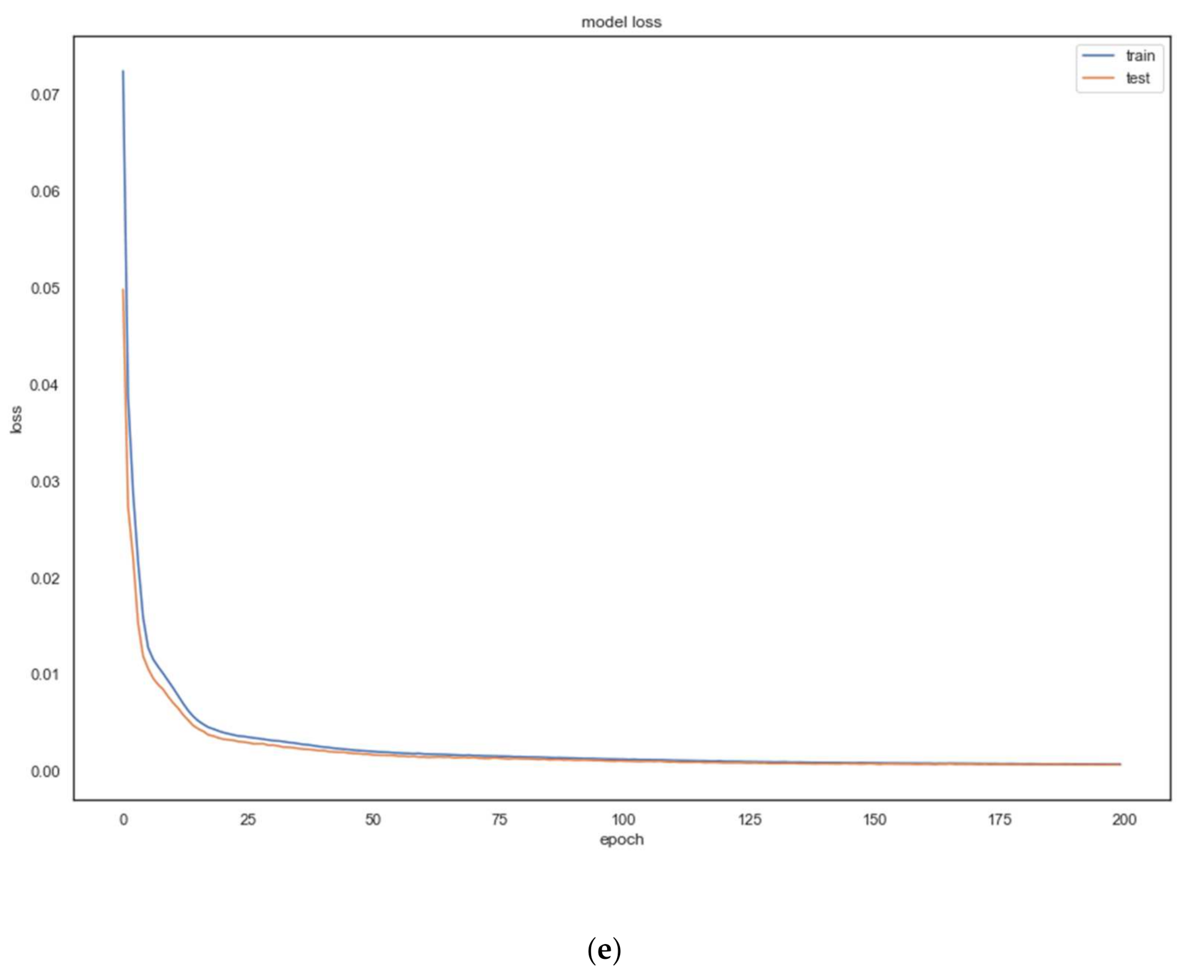
. For some datasets, we increased the number of epochs to test for potential overfitting when the model keeps training. Because of this, the model overfitting is subject to the model’s complexity, especially, in the case of small datasets [69]. However, as can be seen from Figure 3, the reconstruction loss of the AE remains smooth as the model keeps training.

For MLP regressors architecture, we used only one hidden layer of 50 hidden units with ReLU activation function and an output layer of only one output node with linear activation, and we used an adaptive learning rate $\gamma$ initialized at 0.001. The use of the ReLU activation function stemmed from the advantages of ReLU over sigmoidal functions such as sparsity representation and to avoid the saturation problem of sigmoidal activation functions which cause the vanishing gradient problem [70]. We adopted the same MLP architecture for all MLP regressors in the feature mapping network. We adopted an Adam optimizer for backpropagation of the Mean-Squared Error (MSE) for both the autoencoder and the MLP regressors used in the feature mapping network for the ease of hyperparameter tuning. Figure 3 depicts the MSE loss of the autoencoder for each of the five datasets. For the code and implementation details, please refer to Supplementary Materials.

As per our proposed method, we took the Fashion-MNIST dataset as an example of applying our algorithm. We trained the autoencoder with its corresponding architecture (784-512-256-512-784) on the 600 training images (60 samples per class), then we created the Cartesian Product set as in Algorithm 1 using the 600 images in two sets $T{r}_1$ and $T{r}_2$ of size $60\times 59\times 10=\mathrm{35,400}$ data samples.

We then extracted features of $T{r}_1$ and $T{r}_2$ using our trained autoencoder resulting in two matrices of features $Z_1$ and $Z_2$, both of size $\left[\mathrm{35,400}\times 256\right]$. Next, we trained 256 MLP regressors $\left\{ML{P}_1, ML{P}_2, \dots , ML{P}_{256}\right\}$ using $Z_1$ as input and $Z_2$ as target variables, where each MLP regressor takes as input the whole feature vector $z_i\in Z_1$ and learns to output one target feature $z_i^s\in Z, s=1, 2, \dots , 256$, $i=0,1,\dots ,\mathrm{35,400}$. To speed up the training process, we distributed the training of the 256 MLP regressors over eight processes that run in parallel such that each process corresponds to 256/8 = 16 MLP regressors.

Afterwards, we used the trained MLP regressors to double the size of the training set $D^{Tr}$ by transforming the 600 original samples, as shown in Algorithm 2, and augmenting the transformed samples $\widehat{D^{Tr}}$, so we ended up having a training set {$D^{Tr}$, $\widehat{D^{Tr}}$} of 1200 images. We also transformed the original test set $D^{Ts}$ of 69,400 test images resulting in $\widehat{D^{Ts}}$ of 69,400 images as well.

We did the same for all the datasets (each dataset with its AE architecture and hyperparameters as shown in Table 2) and tested our model in two settings, a semi-supervised clustering setting and a classification setting, explained in the next two subsections.

3.2.1. Semi-Supervised Clustering Setting

In the semi-supervised clustering setting, we measured the performance of clustering original test (unlabeled) samples ($D^{Ts}$) (without transformation) and clustering transformed test (unlabeled) samples ($\widehat{D^{Ts}}$) (using our model trained on the few labeled samples). As a clustering algorithm, we used the K-means algorithm [43] with different centroid initialization methods, K-means++ [71], random, and PCA-based (where we calculated the principal component analysis for each sample in the test set and performed the K-means algorithm on the PCA components). We calculated the clustering evaluation metrics, listed below, for each clustering scenario. The experiment is repeated for each test set of the five datasets and results are presented in Table 3. Besides the clustering evaluation metrics, we calculated the clustering time for each scenario (without and with our model).

Clustering Metrics. We used various clustering metrics that relate to within-cluster and between-cluster measures that related to the compactness and separability properties of the targets. The metrics used and their mathematical formulations are listed below.

• Inertia [43]: Within-cluster sum-of-squares criterion.

  $${\displaystyle \sum }_{i=0}^n\underset{{\mu }_j\in C}{\min }\left(‖x_i,-,{\mu }_j‖{}^2\right)$$

  (6)
• Homogeneity, Completeness, and V-Measure [72]: Homogeneity measures a score that each cluster contains only members of a single class. Completeness measures a score that all data points of the same class are assigned to the same cluster. V-Measure measures how successfully homogeneity and completeness have been satisfied.

  $$V_{\beta }=\frac{\left(1+\beta \right)\times H\times C}{\beta \times H+C}$$

  (7)
• Adjusted Rand Index (ARI) [73]: Measures the similarity of two assignments (ground truth and predicted cluster assignment), ignoring permutations.

  $$\mathrm{RI} = \frac{a + b}{C_2^{n_{samples}}}$$

  (8)

  $$ARI=\frac{\mathrm{RI}-E\left[\mathrm{RI}\right]}{\max \left(\mathrm{RI}\right)-E\left[\mathrm{RI}\right]}$$

  (9)
• Adjusted Mutual Information (AMI) [74]: Measures the agreement of two assignments (ground truth and predicted cluster assignment), ignoring permutations. Given two cluster assignments $U$ and $V$, their entropies, mutual information, and adjusted mutual information are defined respectively as:

  $$H\left(U\right)=-{\displaystyle \sum }_{i=1}^{\left|U\right|}P\left(i\right)\log P\left(i\right)$$

  (10)

  where $P\left(i\right)=\left|U_i\right|/N$ is the probability that an object picked from $U$ at random belongs to class $U_i$. Same for $P^{\prime }\left(j\right)$ and $V$.

  $$H\left(V\right)=-{\displaystyle \sum }_{j=1}^{\left|V\right|}{P}^{\prime }\left(j\right)\log P^{\prime }\left(j\right)$$

  (11)

  $$\mathrm{MI}\left(U,V\right)={\displaystyle \sum }_{i=1}^{\left|U\right|}{\displaystyle \sum }_{j=1}^{\left|V\right|}{P}^{″}\left(i,j\right)\log \frac{P^{″}\left(i,j\right)}{P\left(i\right)P^{\prime }\left(j\right)}$$

  (12)

  where $P^{″}\left(i,j\right)=\left|U_i\cap V_j\right|/N$ is the joint probability that an object picked at random belongs to both classes $U_i$ and $V_j$.

  $$\mathrm{AMI}=\frac{\mathrm{MI}-E\left[\mathrm{MI}\right]}{mean\left(H\left(U\right),H\left(V\right)\right)-E\left[\mathrm{MI}\right]}$$

  (13)

  where $E$ is the expected value of the mutual information.
• Silhouette Coefficient [75]: The silhouette coefficient for a single data point is defined as follows:

  $$S=\frac{b-a}{max\left(a,b\right)}$$

  (14)

  where $a$ is the mean distance between the data point and all other points within the same cluster and $b$ is the mean distance between the data point and all other points in the nearest cluster. The mean silhouette coefficient is calculated for all data points, and the higher the score, the better the defined clusters indicating a lower within-cluster distance and a higher between-cluster distance.

As can be seen from Table 3, using our model to map the test set consistently yielded the best results in all clustering performance metrics over all used datasets. An improvement in both the inertia of clusters and the silhouette coefficient indicates that our model achieves its goal of promoting compactness (within-class) and separability (between-class) of data points which subsequently improves all other clustering metrics. Also, using our model to map samples before clustering gives a significant reduction in clustering time of the algorithm, particularly for large datasets (like MNIST and Fashion-MNIST) when applying the K-means++ initialization method.

We also report a comparison to another clustering algorithm (SESSC) [48] on the WDBC dataset. As can be seen from Table 3, their performance on the test set without mapping produces lower values in all calculated clustering metrics relative to using our model on the K-means algorithm with any initialization method. Also, it is noteworthy that applying their algorithm on the mapped test set using our model enhances their performance, which supports our claim that our proposed method is pluggable to any clustering algorithm (hard or soft). We applied their provided code (https://github.com/YuqiCui/SESSC (accessed on 19 January 2022)) on other datasets and followed the guideline for hyperparameter fine tuning mentioned in their paper. However, we were not able to conduct the experiment except for the WDBC dataset. This led to the conclusion that their implementation does not support datasets with relatively high dimensionality.

Table 3. Semi-supervised clustering performance evaluation results. Bolded values indicate the best results achieved in each metric. $D^{Ts}$ is the original unlabeled test set (without transformation) and $\widehat{D^{Ts}}$ is the transformed (using our model) unlabeled test set.

Dataset	K-Means Init. Method	Test Set	$Time$	$Inertia$	$H$	$C$	$V_{\beta }$	$ARI$	$AMI$	$S$
MNIST	K-Means++	$D^{Ts}$	119.802 s	42,141,554	0.421	0.443	0.432	0.322	0.421	0.058
		$\widehat{D^{Ts}}$	32.010 s	14,454,470	0.658	0.680	0.669	0.586	0.658	0.396
	Random	$D^{Ts}$	62.014 s	42,142,078	0.417	0.439	0.428	0.318	0.417	0.060
		$\widehat{D^{Ts}}$	31.006 s	14,454,470	0.658	0.680	0.669	0.586	0.658	0.381
	PCA-Based	$D^{Ts}$	14.302 s	42,142,060	0.417	0.439	0.428	0.317	0.417	0.055
		$\widehat{D^{Ts}}$	8.425 s	14,454,470	0.658	0.680	0.669	0.586	0.658	0.394
Fashion-MNIST	K-Means++	$D^{Ts}$	41.216 s	30,290,316	0.505	0.536	0.520	0.338	0.505	0.151
		$\widehat{D^{Ts}}$	24.270 s	7,065,023	0.705	0.707	0.706	0.636	0.705	0.505
	Random	$D^{Ts}$	44.563 s	30,243,539	0.493	0.518	0.505	0.348	0.493	0.137
		$\widehat{D^{Ts}}$	38.562 s	7,067,789	0.693	0.712	0.702	0.607	0.693	0.510
	PCA-Based	$D^{Ts}$	10.170 s	30,820,962	0.488	0.503	0.495	0.344	0.488	0.131
		$\widehat{D^{Ts}}$	8.454 s	8,803,305	0.675	0.690	0.682	0.587	0.675	0.479
USPS	K-Means++	$D^{Ts}$	1.636 s	1,449,834	0.576	0.583	0.580	0.473	0.575	0.117
		$\widehat{D^{Ts}}$	1.038 s	333,792	0.847	0.848	0.848	0.863	0.847	0.615
	Random	$D^{Ts}$	1.328 s	1,456,828	0.547	0.569	0.558	0.445	0.546	0.118
		$\widehat{D^{Ts}}$	0.889 s	333,788	0.847	0.847	0.847	0.863	0.847	0.571
	PCA-Based	$D^{Ts}$	0.478 s	1,449,824	0.577	0.584	0.580	0.474	0.576	0.119
		$\widehat{D^{Ts}}$	0.197 s	33,793	0.846	0.847	0.847	0.863	0.846	0.621
MSTAR	K-Means++	$D^{Ts}$	3.305 s	9,242,633	0.012	0.016	0.014	0.009	0.009	0.015
		$\widehat{D^{Ts}}$	2.174 s	4,280,437	0.524	0.528	0.526	0.526	0.522	0.388
	Random	$D^{Ts}$	2.142 s	9,232,361	0.017	0.019	0.018	0.009	0.014	0.024
		$\widehat{D^{Ts}}$	1.589 s	4,280,491	0.522	0.527	0.524	0.523	0.520	0.390
	PCA-Based	$D^{Ts}$	0.835 s	9,245,153	0.022	0.023	0.023	0.019	0.019	0.019
		$\widehat{D^{Ts}}$	0.590 s	4,280,491	0.522	0.527	0.524	0.523	0.520	0.371
WDBC	K-Means++	$D^{Ts}$	0.013 s	3454	0.668	0.689	0.678	0.777	0.666	0.391
		$\widehat{D^{Ts}}$	0.010 s	958	0.904	0.904	0.904	0.953	0.904	0.873
	Random	$D^{Ts}$	0.010 s	3454	0.668	0.689	0.678	0.777	0.666	0.391
		$\widehat{D^{Ts}}$	0.008 s	958	0.904	0.904	0.904	0.953	0.904	0.873
	PCA-Based	$D^{Ts}$	0.003 s	3454	0.668	0.689	0.678	0.777	0.666	0.391
		$\widehat{D^{Ts}}$	0.002 s	958	0.904	0.904	0.904	0.953	0.904	0.873
	SESSC	$D^{Ts}$	1.491 s	-	0.871	0.867	0.869	0.930	0.868	0.286
		$\widehat{D^{Ts}}$	1.151 s	-	0.954	0.950	0.952	0.977	0.952	0.711

Table 3. Semi-supervised clustering performance evaluation results. Bolded values indicate the best results achieved in each metric. $D^{Ts}$ is the original unlabeled test set (without transformation) and $\widehat{D^{Ts}}$ is the transformed (using our model) unlabeled test set.

Dataset	K-Means Init. Method	Test Set	$Time$	$Inertia$	$H$	$C$	$V_{\beta }$	$ARI$	$AMI$	$S$
MNIST	K-Means++	$D^{Ts}$	119.802 s	42,141,554	0.421	0.443	0.432	0.322	0.421	0.058
		$\widehat{D^{Ts}}$	32.010 s	14,454,470	0.658	0.680	0.669	0.586	0.658	0.396
	Random	$D^{Ts}$	62.014 s	42,142,078	0.417	0.439	0.428	0.318	0.417	0.060
		$\widehat{D^{Ts}}$	31.006 s	14,454,470	0.658	0.680	0.669	0.586	0.658	0.381
	PCA-Based	$D^{Ts}$	14.302 s	42,142,060	0.417	0.439	0.428	0.317	0.417	0.055
		$\widehat{D^{Ts}}$	8.425 s	14,454,470	0.658	0.680	0.669	0.586	0.658	0.394
Fashion-MNIST	K-Means++	$D^{Ts}$	41.216 s	30,290,316	0.505	0.536	0.520	0.338	0.505	0.151
		$\widehat{D^{Ts}}$	24.270 s	7,065,023	0.705	0.707	0.706	0.636	0.705	0.505
	Random	$D^{Ts}$	44.563 s	30,243,539	0.493	0.518	0.505	0.348	0.493	0.137
		$\widehat{D^{Ts}}$	38.562 s	7,067,789	0.693	0.712	0.702	0.607	0.693	0.510
	PCA-Based	$D^{Ts}$	10.170 s	30,820,962	0.488	0.503	0.495	0.344	0.488	0.131
		$\widehat{D^{Ts}}$	8.454 s	8,803,305	0.675	0.690	0.682	0.587	0.675	0.479
USPS	K-Means++	$D^{Ts}$	1.636 s	1,449,834	0.576	0.583	0.580	0.473	0.575	0.117
		$\widehat{D^{Ts}}$	1.038 s	333,792	0.847	0.848	0.848	0.863	0.847	0.615
	Random	$D^{Ts}$	1.328 s	1,456,828	0.547	0.569	0.558	0.445	0.546	0.118
		$\widehat{D^{Ts}}$	0.889 s	333,788	0.847	0.847	0.847	0.863	0.847	0.571
	PCA-Based	$D^{Ts}$	0.478 s	1,449,824	0.577	0.584	0.580	0.474	0.576	0.119
		$\widehat{D^{Ts}}$	0.197 s	33,793	0.846	0.847	0.847	0.863	0.846	0.621
MSTAR	K-Means++	$D^{Ts}$	3.305 s	9,242,633	0.012	0.016	0.014	0.009	0.009	0.015
		$\widehat{D^{Ts}}$	2.174 s	4,280,437	0.524	0.528	0.526	0.526	0.522	0.388
	Random	$D^{Ts}$	2.142 s	9,232,361	0.017	0.019	0.018	0.009	0.014	0.024
		$\widehat{D^{Ts}}$	1.589 s	4,280,491	0.522	0.527	0.524	0.523	0.520	0.390
	PCA-Based	$D^{Ts}$	0.835 s	9,245,153	0.022	0.023	0.023	0.019	0.019	0.019
		$\widehat{D^{Ts}}$	0.590 s	4,280,491	0.522	0.527	0.524	0.523	0.520	0.371
WDBC	K-Means++	$D^{Ts}$	0.013 s	3454	0.668	0.689	0.678	0.777	0.666	0.391
		$\widehat{D^{Ts}}$	0.010 s	958	0.904	0.904	0.904	0.953	0.904	0.873
	Random	$D^{Ts}$	0.010 s	3454	0.668	0.689	0.678	0.777	0.666	0.391
		$\widehat{D^{Ts}}$	0.008 s	958	0.904	0.904	0.904	0.953	0.904	0.873
	PCA-Based	$D^{Ts}$	0.003 s	3454	0.668	0.689	0.678	0.777	0.666	0.391
		$\widehat{D^{Ts}}$	0.002 s	958	0.904	0.904	0.904	0.953	0.904	0.873
	SESSC	$D^{Ts}$	1.491 s	-	0.871	0.867	0.869	0.930	0.868	0.286
		$\widehat{D^{Ts}}$	1.151 s	-	0.954	0.950	0.952	0.977	0.952	0.711

3.2.2. Classification Setting

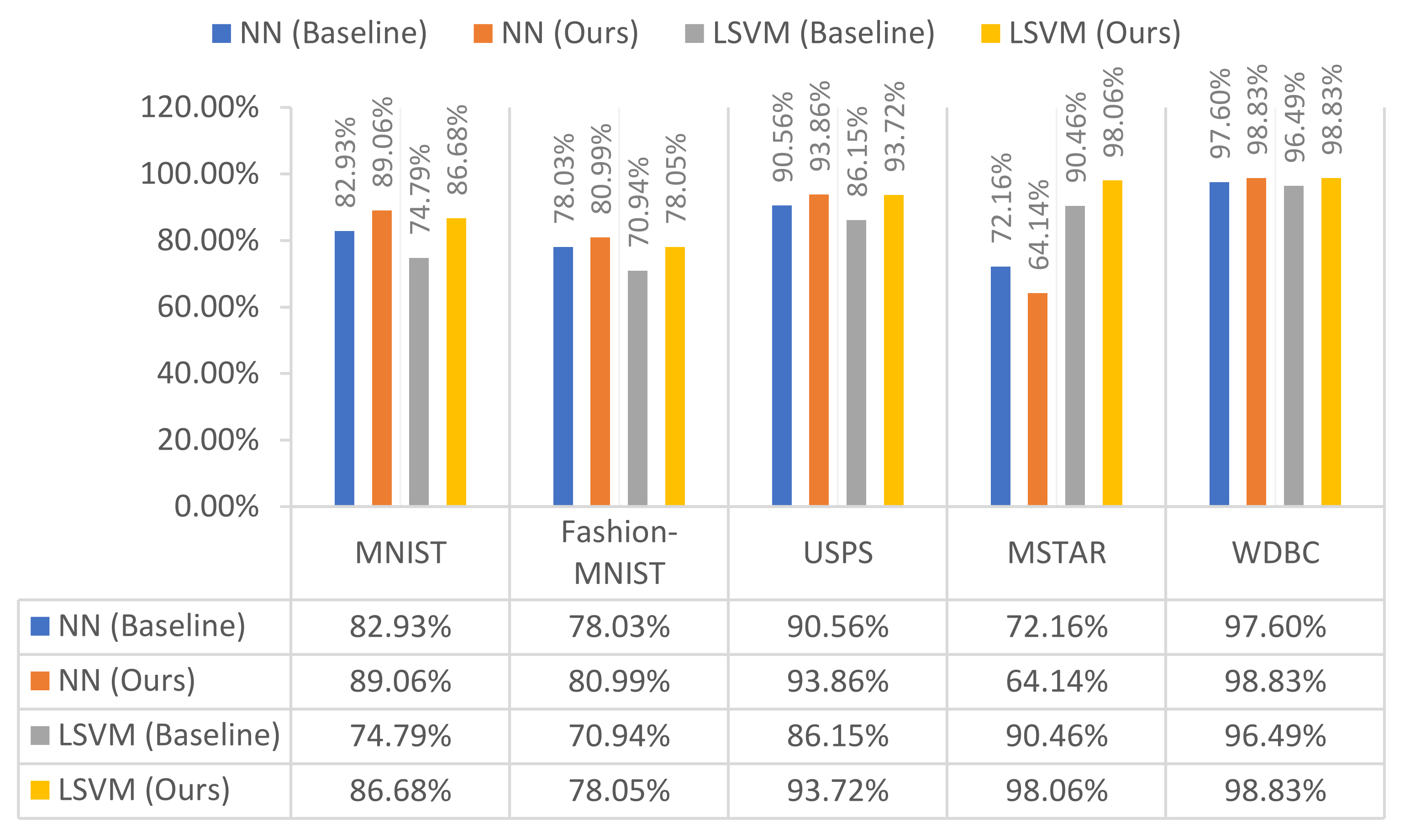
We devised an experiment where we employ our model before training a classifier to map both the training set and the test set. We then trained the classifier on the plain training set ($D^{Tr}$) augmented with the mapped training set ($\widehat{D^{Tr}}$) using our model, and we evaluated the classifier on the mapped test set ($\widehat{D^{Ts}}$). We compared our experiment with a baseline experiment where we trained the classifier on the plain training set ($D^{Tr}$) and evaluated it on the plain test set ($D^{Ts}$).

We deployed a neural network (NN) and a linear SVM models for the classification task. We used a linear SVM as a classifier because improving accuracy with a linear classifier demonstrates the linear separability enhancement of transformed data points. We measured the accuracy for both classifier models (NN and LSVM) and the loss for the NN model. Experiments were repeated 10 times independently and average accuracy and average loss was calculated over the 10 runs for each experiment and compare the obtained results of the baseline experiment against ours. Both experiments with both classifiers were run for the five datasets and results are listed in

Table 4. Classification results. $D^{Tr}$ is the original training set (without transformation) and {$D^{Tr}$, $\widehat{D^{Tr}}$} is the original training $D^{Tr}$ set augmented with the transformed (using our model) training set $\widehat{D^{Tr}}$. Bolded values indicate the best results achieved in each metric.

Dataset	Classifier	Train Set	Test Set	Average Accuracy	Average Loss
MNIST	NN	$D^{Tr}$	$D^{Ts}$	0.829278	0.588378
		$\{D^{Tr}$$, \widehat{D^{Tr}}$}	$\widehat{D^{Ts}}$	0.890600	0.423493
	LSVM	$D^{Tr}$	$D^{Ts}$	0.747853	-
		$\{D^{Tr}$$, \widehat{D^{Tr}}$}	$\widehat{D^{Ts}}$	0.866773	-
Fashion-MNIST	NN	$D^{Tr}$	$D^{Ts}$	0.780324	0.652228
		$\{D^{Tr}$$, \widehat{D^{Tr}}$}	$\widehat{D^{Ts}}$	0.809889	0.648123
	LSVM	$D^{Tr}$	$D^{Ts}$	0.709376	-
		$\{D^{Tr}$$, \widehat{D^{Tr}}$}	$\widehat{D^{Ts}}$	0.780488	-
USPS	NN	$D^{Tr}$	$D^{Ts}$	0.905552	0.328199
		$\{D^{Tr}$$, \widehat{D^{Tr}}$}	$\widehat{D^{Ts}}$	0.938645	0.245099
	LSVM	$D^{Tr}$	$D^{Ts}$	0.861530	-
		$\{D^{Tr}$$, \widehat{D^{Tr}}$}	$\widehat{D^{Ts}}$	0.937175	-
MSTAR	NN	$D^{Tr}$	$D^{Ts}$	0.721635	0.528935
		$\{D^{Tr}$$, \widehat{D^{Tr}}$}	$\widehat{D^{Ts}}$	0.641397	0.620295
	LSVM	$D^{Tr}$	$D^{Ts}$	0.904600	-
		$\{D^{Tr}$$, \widehat{D^{Tr}}$}	$\widehat{D^{Ts}}$	0.980579	-
WDBC	NN	$D^{Tr}$	$D^{Ts}$	0.976023	0.101761
		$\{D^{Tr}$$, \widehat{D^{Tr}}$}	$\widehat{D^{Ts}}$	0.988304	0.034921
	LSVM	$D^{Tr}$	$D^{Ts}$	0.964912	-
		$\{D^{Tr}$$, \widehat{D^{Tr}}$}	$\widehat{D^{Ts}}$	0.988304	-
	ESSC_LSE	$D^{Tr}$	$D^{Ts}$	0.949708	-
		$\{D^{Tr}$$, \widehat{D^{Tr}}$}	$\widehat{D^{Ts}}$	0.985965	-
	SESSC	$D^{Tr}$	$D^{Ts}$	0.954386	-
		$\{D^{Tr}$$, \widehat{D^{Tr}}$}	$\widehat{D^{Ts}}$	0.992398	-
	SESSC_LSE	$D^{Tr}$	$D^{Ts}$	0.971930	-
		$\{D^{Tr}$$, \widehat{D^{Tr}}$}	$\widehat{D^{Ts}}$	0.990058	-

and illustrated in Figure 4. From the results, one can observe that the accuracy of both the neural network and the linear SVM classifiers are enhanced in nearly all the datasets. Also, we can see that the LSVM classifier’s accuracies with our model are on par with the NN classifier which indicates that the linear separability is enhanced because of our model. We can observe that the SVM classifier outperforms the NN classifier on the MSTAR dataset in both settings, with and without our model. A plausible explanation for why the NN classifier performs poorly on such a dataset is that NN classifiers suffer when the input data dimensionality is high. This drawback of NN classifiers is relatively remedied when the number of training samples is adequately large relative to the number of parameters preventing the plausible overfitting [76]. This is unfortunately not available in our case of small datasets, especially the MSTAR dataset. On the other hand, SVM training requires a much smaller number of data samples as they rely on the support vectors which is a very small subset of the training samples. We also conducted experiments on classifiers used in [48] and added their results on the WDBC dataset in Table 4. The used classifiers were SESSC as a standalone classifier, ESSC_LSE, and SESSC_LSE (the ESSC and the SESSC clustering algorithms integrated with a fuzzy classifier, respectively). We can notice that again using our model to transform the test set improves their performance as other classifiers, which further proves the pluggable feature of our model.

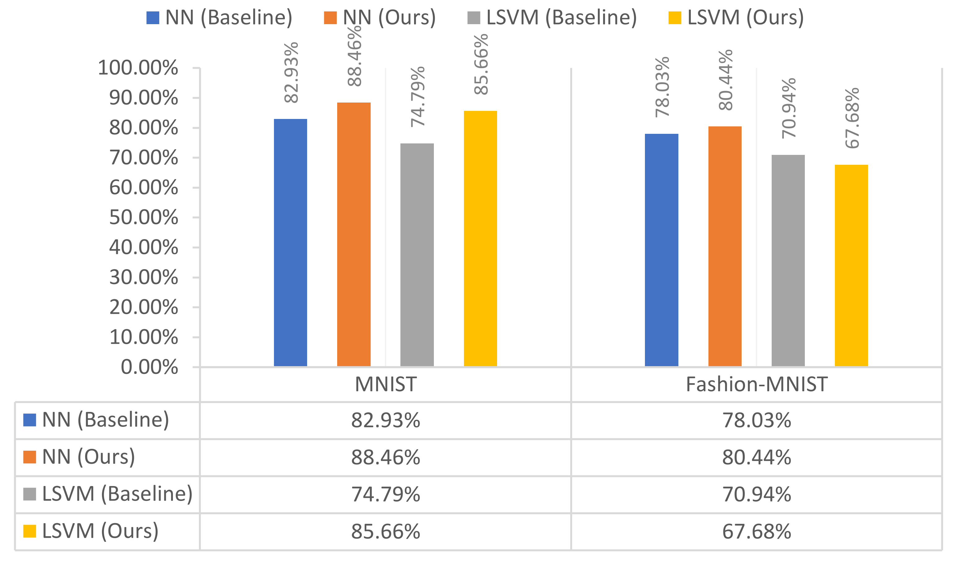
In addition to the proposed classification setting, we undertook a set of pilot experiments on a limited number of the used datasets. In Set-1 of the pilot experiments, we trained the classifier on only $D^{Tr}$ (without augmenting $\widehat{D^{Tr}}$) and tested its performance on the transformed test set $\widehat{D^{Ts}}$. Although our pilot experiment improved the classifier performance in most of the datasets, we found that training the classifier with the augmented set consistently gave better results over all datasets since augmentation increased the size of the training set which reduced the classifier overfitting. Also, adding the transformed samples to the training pool helps the classifier to achieve better decision boundaries relative to the transformed test samples $\widehat{D^{Ts}}$ as it was trained on the transformed training samples before, which makes it achieve better results. A summary of the pilot experiment results is presented in

Table 5. Set-1 pilot experiment results. $D^{Tr}$ is the original training set (without transformation), $D^{Ts}$ is the original unlabeled test set (without transformation), and $\widehat{D^{Ts}}$ is the transformed (using our model) unlabeled test set. Bolded values indicate the best results achieved in each metric.

Dataset	Classifier	Train Set	Test Set	Average Accuracy	Average Loss
MNIST	NN	$D^{Tr}$	$D^{Ts}$	0.829278	0.588378
		$D^{Tr}$	$\widehat{D^{Ts}}$	0.884564	0.409574
	LSVM	$D^{Tr}$	$D^{Ts}$	0.747853	-
		$D^{Tr}$	$\widehat{D^{Ts}}$	0.856637	-
Fashion-MNIST	NN	$D^{Tr}$	$D^{Ts}$	0.780324	0.652228
		$D^{Tr}$	$\widehat{D^{Ts}}$	0.804369	0.593578
	LSVM	$D^{Tr}$	$D^{Ts}$	0.709376	-
		$D^{Tr}$	$\widehat{D^{Ts}}$	0.676829	-

and Figure 5.

In Set-2 of the pilot experiments, we compared two options. Option 1 was using the reconstructions of the third module as input to the classifier versus the original input data (as demonstrated before). Option 2 was proceeding to the applied classifier with the output of the second module, which were the latent representations obtained from the regressors, versus using the latent representations obtained directly from the autoencoder. Results for semi-supervised clustering and classification are shown in

Table 6. Set-2 pilot experiment semi-supervised clustering setting results. $D^{Ts}$ is the original unlabeled test set (without transformation), $\widehat{D^{Ts}}$ is the transformed (using our model) unlabeled test set. $Z_{ts}$ and $\widehat{Z_{ts}}$ are the features extracted from the autoencoder of the original test set $D^{Ts}$ and the transformed test set $\widehat{D^{Ts}}$, respectively. Bolded values indicate the best results achieved in each metric.

Dataset	K-Means Init. Method	Option	Test Set	$Time$	$Inertia$	$H$	$C$	$V_{\beta }$	$ARI$	$AMI$	$S$
MNIST	K-Means++	Option1	$D^{Ts}$	119.802 s	42,141,554	0.421	0.443	0.432	0.322	0.421	0.058
			$\widehat{D^{Ts}}$	32.010 s	14,454,470	0.658	0.680	0.669	0.586	0.658	0.396
		Option2	$Z_{ts}$	19.931 s	14,528,156	0.537	0.544	0.541	0.418	0.537	0.063
			$\widehat{Z_{ts}}$	15.100 s	6,730,338	0.666	0.676	0.671	0.570	0.666	0.329
	Random	Option1	$D^{Ts}$	62.014 s	42,142,078	0.417	0.439	0.428	0.318	0.417	0.060
			$\widehat{D^{Ts}}$	31.006 s	14,454,470	0.658	0.680	0.669	0.586	0.658	0.381
		Option2	$Z_{ts}$	18.312 s	14,510,545	0.526	0.535	0.531	0.397	0.526	0.066
			$\widehat{Z_{ts}}$	11.168 s	6,730,342	0.666	0.676	0.671	0.570	0.666	0.329
	PCA-Based	Option1	$D^{Ts}$	14.302 s	42,142,060	0.417	0.439	0.428	0.317	0.417	0.055
			$\widehat{D^{Ts}}$	8.425 s	14,454,470	0.658	0.680	0.669	0.586	0.658	0.394
		Option2	$Z_{ts}$	4.908 s	14,510,560	0.526	0.535	0.531	0.397	0.526	0.062
			$\widehat{Z_{ts}}$	3.618 s	6,847,240	0.655	0.664	0.659	0.567	0.655	0.262
Fashion-MNIST	K-Means++	Option1	$D^{Ts}$	41.216 s	30,290,316	0.505	0.536	0.520	0.338	0.505	0.151
			$\widehat{D^{Ts}}$	24.270 s	7,065,023	0.705	0.707	0.706	0.636	0.705	0.505
		Option2	$Z_{ts}$	14.065 s	12,138,071	0.506	0.523	0.515	0.315	0.506	0.103
			$\widehat{Z_{ts}}$	9.982 s	4,670,369	0.674	0.677	0.676	0.588	0.674	0.325
	Random	Option1	$D^{Ts}$	44.563 s	30,243,539	0.493	0.518	0.505	0.348	0.493	0.137
			$\widehat{D^{Ts}}$	38.562 s	7,067,789	0.693	0.712	0.702	0.607	0.693	0.510
		Option2	$Z_{ts}$	18.293 s	12,179,589	0.510	0.524	0.517	0.331	0.510	0.084
			$\widehat{Z_{ts}}$	10.308 s	4,670,369	0.674	0.677	0.676	0.588	0.674	0.355
	PCA-Based	Option1	$D^{Ts}$	10.170 s	30,820,962	0.488	0.503	0.495	0.344	0.488	0.131
			$\widehat{D^{Ts}}$	8.454 s	8,803,305	0.675	0.690	0.682	0.587	0.675	0.479
		Option2	$Z_{ts}$	3.447 s	12,274,965	0.514	0.530	0.522	0.361	0.514	0.100
			$\widehat{Z_{ts}}$	2.250 s	5,529,373	0.644	0.663	0.653	0.531	0.643	0.329

and

Table 7. Set-2 pilot experiment classification setting results. Bolded values indicate the comparison result between the two options. $D^{Tr}$ is the original training set (without transformation) and {$D^{Tr}$, $\widehat{D^{Tr}}$} is the original training $D^{Tr}$ set augmented with the transformed (using our model) training set $\widehat{D^{Tr}}$. {$Z_{tr}$, $\widehat{Z_{tr}}$} is the features extracted from the autoencoder of the original training set $D^{Tr}$ augmented with the extracted features of the transformed training set $\widehat{D^{Tr}}$, respectively.

Dataset	Classifier	Option	Train Set	Test Set	Average Accuracy	Average Loss
MNIST	NN	Option1	$D^{Tr}$	$D^{Ts}$	0.829278	0.588378
		Option2	$Z_{tr}$	$Z_{ts}$	0.817143	0.728606
		Option1	$\{D^{Tr}$$, \widehat{D^{Tr}}$}	$\widehat{D^{Ts}}$	0.890600	0.423493
		Option2	$\{Z_{tr}$$, \widehat{Z_{tr}}$}	$\widehat{Z_{ts}}$	0.881613	0.415675
	LSVM	Option1	$D^{Tr}$	$D^{Ts}$	0.747853	-
		Option2	$Z_{tr}$	$Z_{ts}$	0.817158	-
		Option1	$\{D^{Tr}$$, \widehat{D^{Tr}}$}	$\widehat{D^{Ts}}$	0.866773	-
		Option2	$\{Z_{tr}$$, \widehat{Z_{tr}}$}	$\widehat{Z_{ts}}$	0.736704	-
Fashion-MNIST	NN	Option1	$D^{Tr}$	$D^{Ts}$	0.780324	0.652228
		Option2	$Z_{tr}$	$Z_{ts}$	0.782837	0.770872
		Option1	$\{D^{Tr}$$, \widehat{D^{Tr}}$}	$\widehat{D^{Ts}}$	0.809889	0.648123
		Option2	$\{Z_{tr}$$, \widehat{Z_{tr}}$}	$\widehat{Z_{ts}}$	0.808163	0.728820
	LSVM	Option1	$D^{Tr}$	$D^{Ts}$	0.709376	-
		Option2	$Z_{tr}$	$Z_{ts}$	0.763546	-
		Option1	$\{D^{Tr}$$, \widehat{D^{Tr}}$}	$\widehat{D^{Ts}}$	0.780488	-
		Option2	$\{Z_{tr}$$, \widehat{Z_{tr}}$}	$\widehat{Z_{ts}}$	0.800102	-

, respectively. Bolded values indicate the best results obtained in each metric except for Inertia where bolded value indicate the best results obtained for each option separately as Inertia is not a normalized metric. The results show that Option 1 is slightly better than Option 2 in most cases in both semi-supervised and supervised settings. In addition, the reconstruction option has the added privilege of not interfering with any subsequent machine learning task. Because the output is of the same dimensionality and nature of the input data, (i.e., no changes are needed for the baseline classification and clustering model setups).

In addition, to further prove the effectiveness of our proposed method, we have provided a comparison with different conventional methods that work on the improvement of classification accuracy of the two naturally small datasets used in this research (WDBC and MSTAR). First, we compared the WDBC dataset to other existing methods that improve the classification accuracy over the dataset using different techniques, mostly feature selection. The WDBC dataset was first normalized and then split into 70–30% training and testing sets. The comparison results are shown in

Table 8. The WDBC dataset comparison results of the proposed method with other methods. The results are sorted in descending order. Bolded values are the results obtained from this study.

Method	Classification Accuracy
Rahman et al. [77]	99.40%
Proposed Method + SESSC	99.23%
Proposed Method + LSVM	98.83%
Yoon et al. [78]	98.80%
Zhang et al. [79]	98.36%
Murugan et al. [80]	98.19%
Nekkaa et al. [81]	97.88%
Aalaei et al. [82]	97.30%
Mafarja et al. [83]	97.10%
Azhagusundari et al. [84]	73.78%

. As can be seen from the table, our proposed method achieves the second highest accuracy which exhibits the model’s effectiveness on this dataset.

We also compared our MSTAR three-target classification accuracy result (98.06%) with other research done on classification accuracy enhancement on the same dataset. We compared with some conventional methods that do not employ data augmentation such as [85] that uses a joint sparse representation (JRS) model, [86] which makes use of phase and amplitude as well as image data, a sparse representation classifier, and Riemannian manifolds, Euclidean distance restricted autoencoder [87], and a hierarchical recognition system that is based on a constrained restricted Boltzmann machine (RBM) [88]. In addition, we included a method that uses data augmentation (deep learning method based on visual cortical system [89]). The comparison results presented in

Table 9. The MSTAR three-target dataset comparison results of the proposed method with other methods. The results are sorted in descending order. Bolded value is the result of this study.

Method	Classification Accuracy
Proposed Method + LSVM	98.06%
Ni et al. [89] (With Data Augmentation)	96.70%
Dong et al. [86]	96.10%
Cui et al. [88]	95.31%
Deng et al. [87]	94.14%
Zhang et al. [85]	93.20%
Ni et al. [89] (Without Data Augmentation)	92.10%

show that the LSVM using our model achieves a comparable accuracy to other research results; also, it is worth noting the effect of data augmentation on classification accuracy such as in [89] where using data augmentation enhances the classification accuracy by 4.6%.

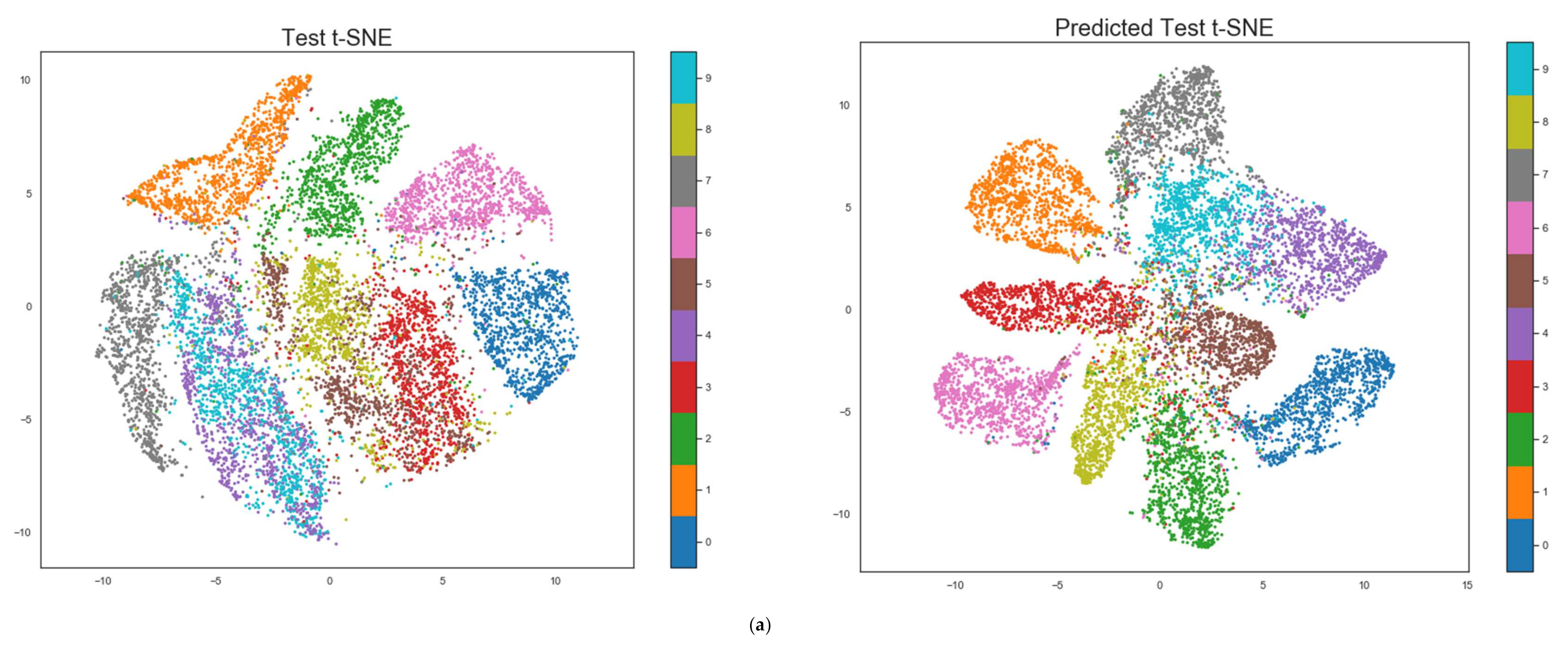
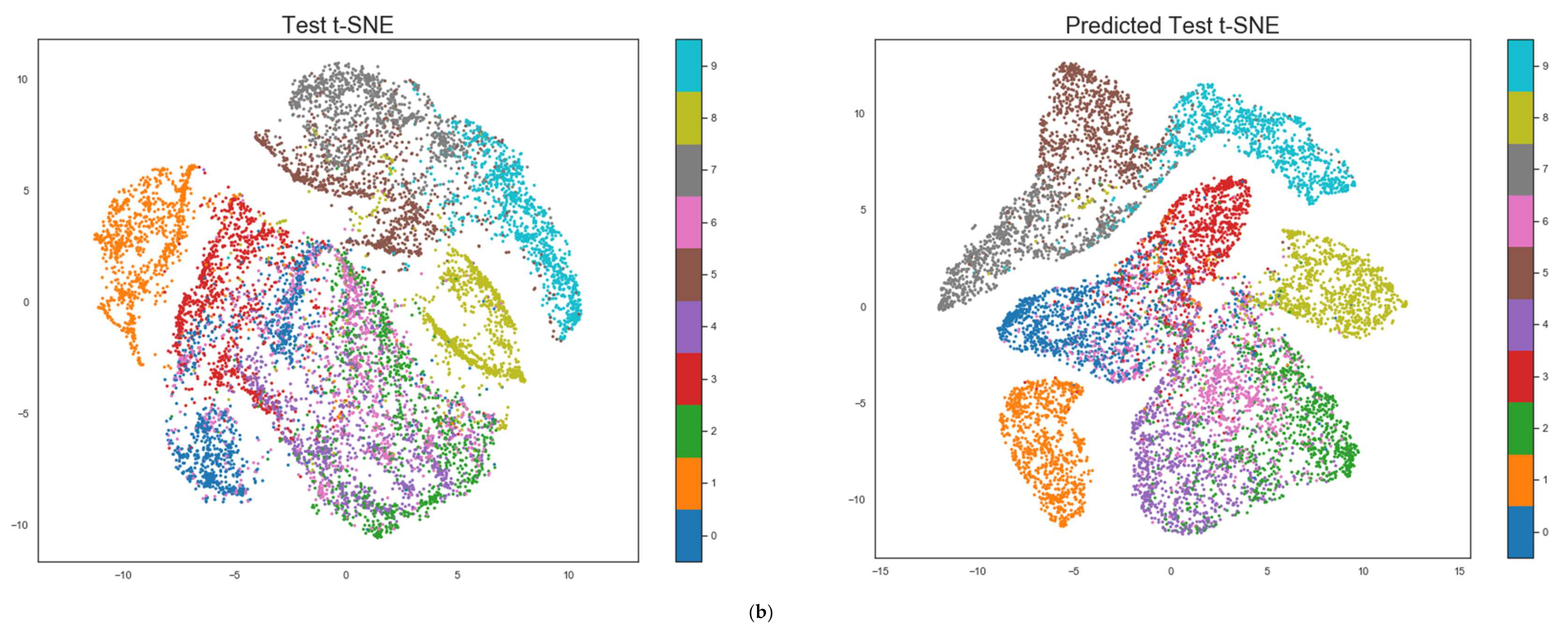
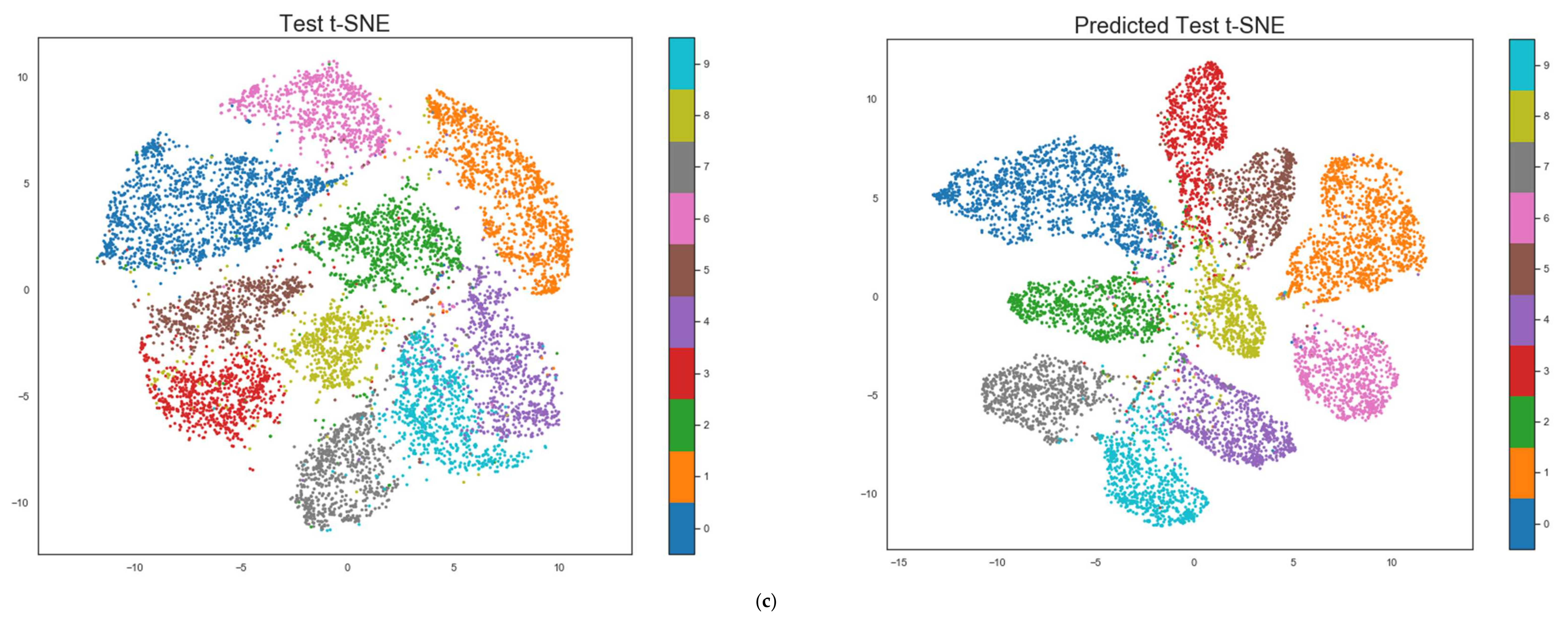
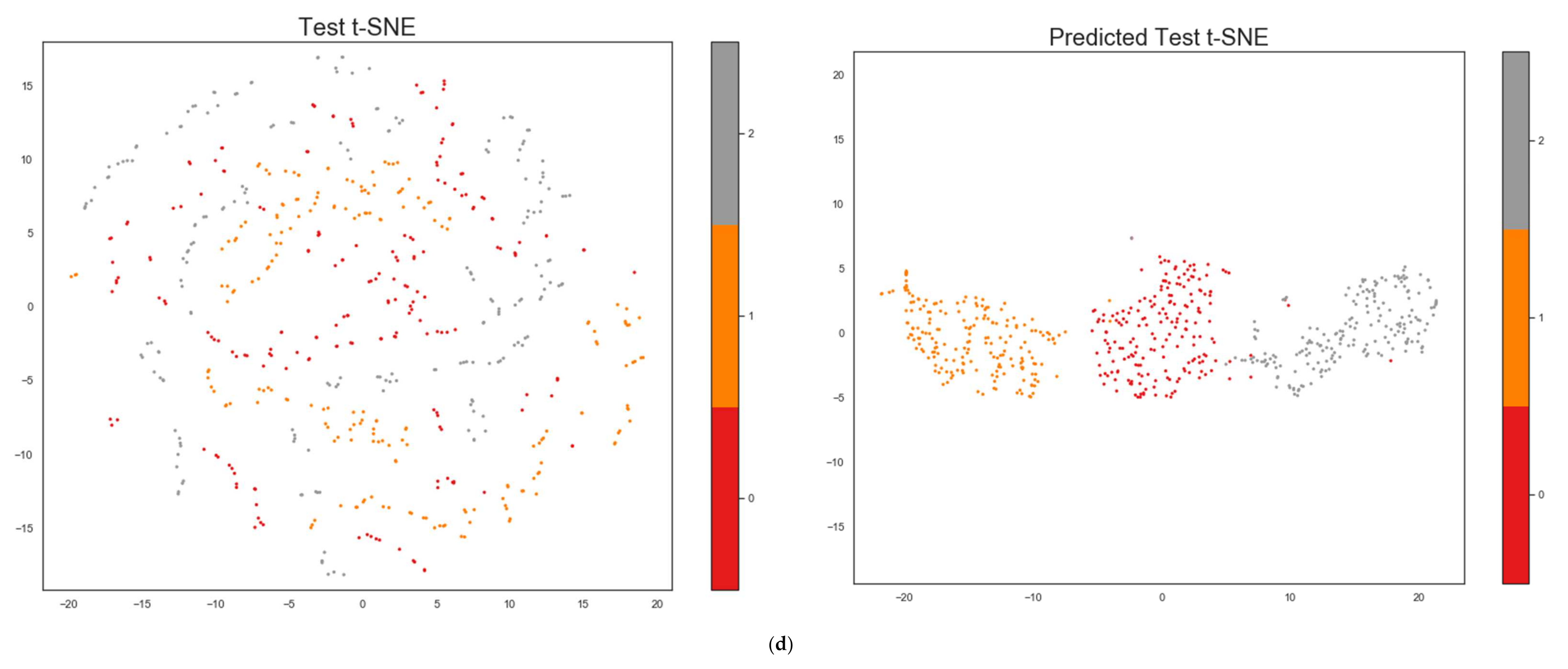
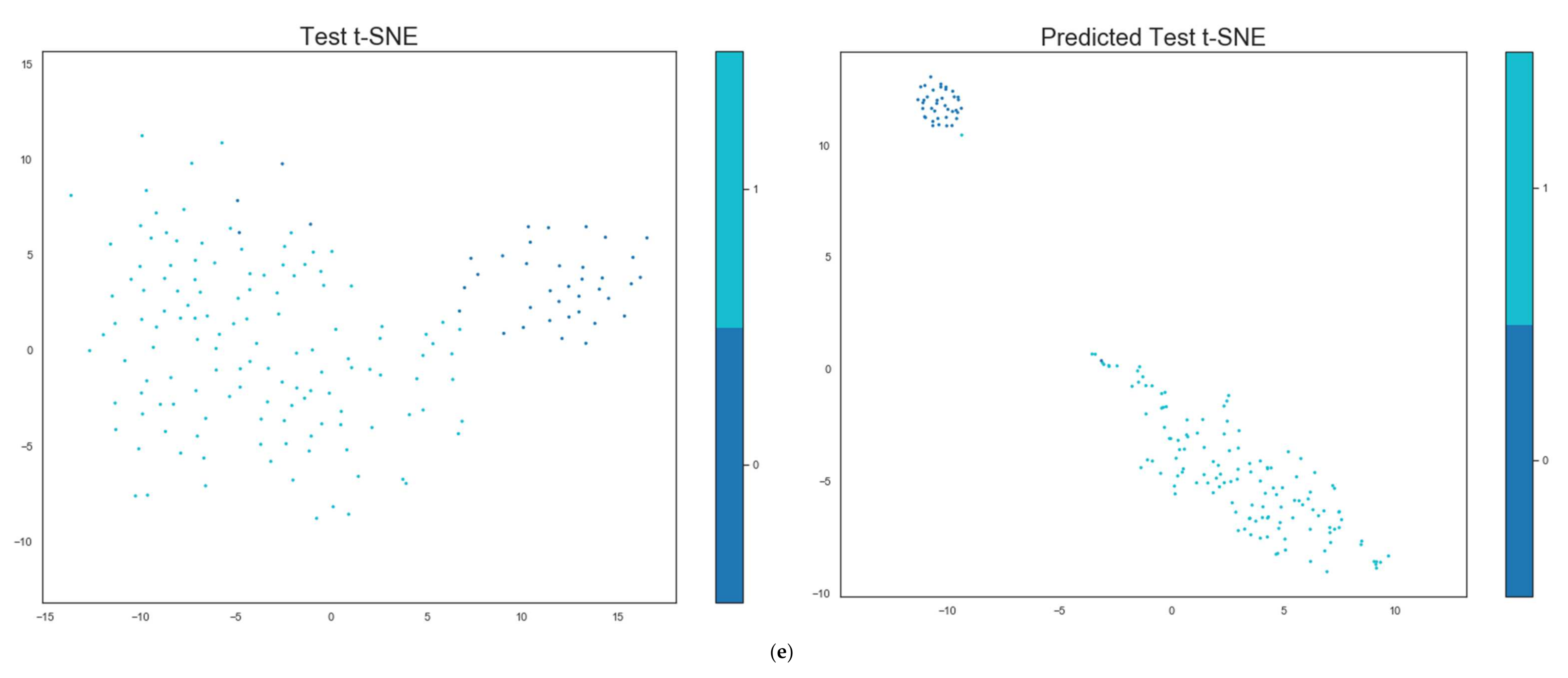
Besides the quantitative results that demonstrate our model’s ability to improve the compactness and separability properties, we show qualitative results through visualizing the mapped features in the feature space using t-SNE [90]. Figure 6 depicts the t-SNE of the plain test set vs. the mapped test set for the five datasets. One can observe that the classes are more separable and compact, especially overlapped classes as, for example, shown by the digits 4 and 9 in the MNIST dataset (highlighted in red circles).

4. Conclusions

This paper proposes a framework that has the potential to improve the compactness and separability properties of data points, which consistently boosts the performance of any off-the-shelf classifier, or a semi-supervised clustering model. We have utilized the generative capacity of autoencoders to reconstruct data points, thus preserving the original input feature space. This characteristic of our proposed framework makes it easily pluggable before a classifier model (not limited by a specific classifier type) or semi-supervised clustering model. We have also utilized an array of MLP regressors for mapping the latent representation of the input samples to approximations of the centroids of the classes. We conducted experiments on five different datasets (MNIST, Fashion-MNIST, USPS, MSTAR, and WDBC) to demonstrate the results of our proposed method. We concluded that plugging our model as a preprocessing step gives better results in all the datasets in both classification and semi-supervised clustering tasks. We also compared the proposed method to other existing methods on enhancing the classification accuracy over the WDBC and MSTAR datasets. We illustrated the importance of augmenting small datasets with the produced approximation of the centroids of the classes and how it further improves the classifier results.