Investigating Explainability Methods in Recurrent Neural Network Architectures for Financial Time Series Data

Abstract

Statistical methods were traditionally primarily used for time series forecasting. However, new hybrid methods demonstrate competitive accuracy, leading to increased machine-learning-based methodologies in the financial sector. However, very little development has been seen in explainable AI (XAI) for financial time series prediction, with a growing mandate for explainable systems. This study aims to determine if the existing XAI methodology is transferable to the context of financial time series prediction. Four popular methods, namely, ablation, permutation, added noise, and integrated gradients, were applied to a recurrent neural network (RNN), long short-term memory (LSTM), and a gated recurrent unit (GRU) network trained on S&P 500 stocks data to determine the importance of features, individual data points, and specific cells in each architecture. The explainability analysis revealed that GRU displayed the most significant ability to retain long-term information, while the LSTM disregarded most of the given input and instead showed the most notable granularity to the considered inputs. Lastly, the RNN displayed features indicative of no long-term memory retention. The applied XAI methods produced complementary results, reinforcing paradigms on significant differences in how different architectures predict. The results show that these methods are transferable in the financial forecasting sector, but a more sophisticated hybrid prediction system requires further confirmation.

1. Introduction

Artificial intelligence (AI) is increasingly becoming an integral part of society, and is applied in fields ranging from finance to healthcare and computer vision [1,2,3]. However, there is an inverse relationship between explainability in a system and its predictive accuracy [4]. Consequently, neural networks and deep learning, which offer the highest accuracy for tasks such as natural language processing and computer vision, are also the least interpretable. Equally, their inherent complexity and nonlinear nature enable such models to learn abstract patterns whilst leading to difficulties in explaining their predictions. As a result, researchers have classed such methods as being a “black box”, which runs the risks of perpetuating computer-based discrimination and bias [5]. Furthermore, in the worst-case scenario, failing to understand how an AI system may function could lead to physical harm as AI becomes further integrated into society [6]. Recognising the necessity of explainable AI (XAI) has seen a concerted effort by governments to implement laws concerning the implementation of explainable prediction systems [7].

Notably, XAI has seen significant use and advancement in computer vision and natural language processing, since it allows one to contrast how machines and humans learn. Opaque models, such as neural networks, are those requiring post hoc analyses in order to achieve explainability. Such post hoc analyses can further be divided into model-agnostic and model-specific [8,9]. Currently, the Shapley additive explanations (SHAP) and local interpretable model-agnostic explanations (LIME) values are foremost choices when it comes to agnostic XAI methods [10,11]. Practitioners commonly use these methods to generate counterfactual explanations that describe the necessary changes required in an input to change a classification [12]. While LIME and SHAP are desirable for their model-agnostic property, researchers have also observed success among model-specific XAI methods.

Recent advances in time series XAI methods focus on convolutional neural networks (CNN) applications. The XCM algorithm developed by Fauvel et al. provides insights behind feature importance through time and feature attribution maps in various health data [13]. This algorithm boasts granularity in both global and local explainability and is based on gradient-weighted class activation mapping (Grad-CAM) [14]. Additionally, Viton et al. similarly incorporated the use of a CNN to generate heatmaps to describe feature and time importance surrounding the decline of patients in health datasets [15]. Both methods demonstrate the practicality of CNN in determining feature importance in deep classification networks. However, these methods prove ineffective for financial time series forecasting. The methods are either not applicable to time series data or are directed towards classification algorithms, further highlighting the need for XAI methods for financial forecasting models. In devising such an algorithm, insight can be gained from examining XAI methods used in other fields.

Ablation is one of the first local explainability methods used in computer vision. Ablation infers image pixel importance by measuring the change in prediction when removing information from a region [16]. Similar to LIME, ablation is a local method that explains a specific prediction for a given input. However, ablation carries the disadvantage that the size and shape of the ablation pattern may lead to false positive and false negative in determining importance among features. Furthermore, the ablation pattern may fail to account for feature interactions [17]. The integrated gradients approach uses backpropagation of attributions of the image against a blank baseline to improve the ablation method. Similar to the blanked region in ablation, this baseline means to represent a state of no information. By noting the change in gradients between the baseline and the standard input and scaling against the input, it allows the identifications of informative features and, in doing so, removes the noise generated by the ablation method [18]. In contrast to these two methods, global explainability methods seek to explain which factors are essential for all predictions of a given system. The permutation method is such a method where the relative importance is determined based on the degree of change experienced in all predictions after single feature values are randomised [19].

Researchers have made less progress in explainable financial time series forecasting despite the diversity and improvement of explainability methods [20]. The slow progress in XAI research in time series forecasting stems from the previous lack of necessity, as inherently explainable statistical methods see preferential use over machine learning methods [21,22]. The delayed uptake of XAI methods in financial forecasting is apparent when considering the limited recently published methods pertaining to regression rather than classification problems [23,24]. Furthermore, existing time series XAI methods may not apply to financial forecasting; here, the aim of XAI is often to determine if models, prone to backtest overfitting, are fitting patterns that are random noise [25]. Among the machine learning techniques for forecasting, practitioners often employ RNN architectures [26,27]. This preference is because they perform reasonably for sequential data, despite in many instances being overshadowed by exponential smoothing and autoregressive methods [28,29]. However, recent results suggest that an ensemble of purely deep learning methods provide a more accurate means of prediction, which has led to an increased usage of neural-network-based forecasting strategies [30,31]. As it stands, financial time series forecasting lags other fields in explainability in the number of available methods and use in industry, making application of these state-of-the-art methods difficult in conforming to current XAI governance policies [20].

The lack of progress in explainable forecasting raises the question of whether existing XAI methodologies are transferable to the financial time series forecasting context or if novel methods are needed. In addressing this question, the research presented here aims to establish a baseline for XAI in time series forecasting using existing methods in the hope of guiding future efforts into more accurate and context-specific XAI methods. In doing so, this study will support the uptake of increasingly accurate “black box” machine-learning forecasting methods by providing additional means to comply with XAI policies.

This paper explores the feasibility of using established explainability methods, namely ablation, permutation, random noise, and integrated gradients, within the context of financial prediction and RNN architectures. Specifically, the baseline RNN, LSTM, and a GRU form the focus of this study. The results presented here demonstrate that existing XAI techniques are transferable to financial time series forecasting RNN architectures, providing insight into how each model makes predictions.

The presented analysis provides evidence for the applicability among existing XAI methods in financial time series forecasting, providing robust complementary results. Furthermore, we have outlined an alteration to the random noise method more applicable to recurrent neural network architectures. Collectively, these results form a baseline for future research aimed at developing methods specific to explainable time series forecasting machine learning strategies.

2. Materials and Methods

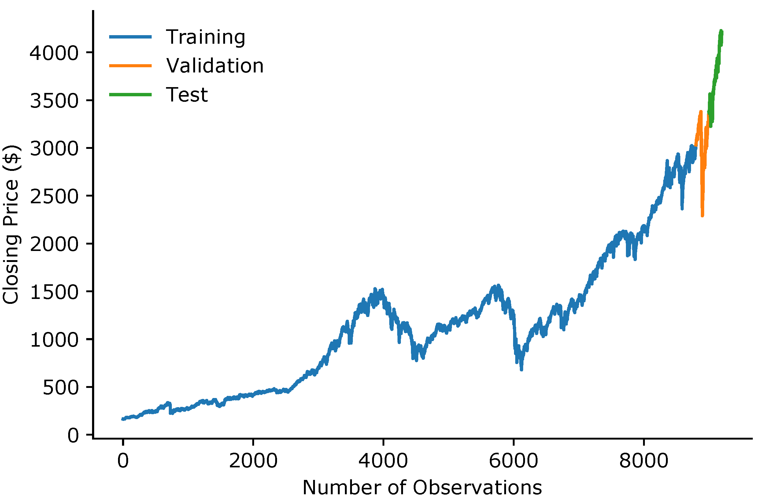
2.1. Dataset and Processing

We constructed the multivariate time series ${\mathbf{T}}_{l;f}$ from the daily S&P 500 between 2 December 1984 and 28 May 2021, excluding weekends, spanning $l=9197$ days. Each day contains $f=6$ features representing the opening, closing, adjusted closing, maximum price, minimum price, and volume traded for the day for each asset. Subsequently, the trend was removed through seasonal and trend decomposition using local regression (LOESS). The augmented Dickey–Fuller test confirmed if the time series was stationary before it underwent global normalization [32].

Additionally, as shown in Figure 1, the data were split into training, validation, and test dataset, where the validation and test datasets constituted the last 400 data points, split evenly between them. Furthermore, the last 99 values of the training dataset were prepended to the validation set to allow for the prediction of the first validation value. The inclusion of the preceding 99 values of the validation set was repeated in the test dataset to allow for the same predictions.

2.2. Models

The study used three different recurrent neural network architectures as models to investigate explainability methods: a standard RNN, a GRU, and an LSTM. Hyperparameters (# hidden states, # layers(cells), dropout and alpha) were optimised using Adam, minimising the mean-squared error on the validation set [33,34]. As shown in Figure 2, the networks follow the same general structure. The models used $w=92$ time steps as an input window, representing a financial quarter. The models forecast the closing price $\widehat{y}$ at a horizon $h=7$ days in the future.

We trained the models for 30 epochs with minibatches of size 3000. After that, we evaluated model performance using the symmetric mean absolute percentage error (SMAPE):

$$\frac{2}{n}\sum _{i=1}^n\frac{|Y_i-{\widehat{Y}}_i|}{|Y_i|+|{\widehat{Y}}_i|}$$

(1)

where $Y_i$ is the actual value and ${\widehat{Y}}_i$ is the predicted value over n predictions. Despite the differences in the parameters among the models, the models were comparable in accuracy, as shown in

Table 1. Hyperparameters and test accuracy for the various RNN architectures.

Model	Hidden States	Layers (# Cells)	Dropout	Alpha	Test Accuracy (SMAPE)
RNN	64	1	0.000	0.005	1.83
GRU	128	2	0.065	0.010	1.81
LSTM	128	2	0.050	0.008	1.81

.

2.3. Ablation

Ablation studies use regions of noninformation to determine significant data points in an input. In RNNs, zeroing of input can be achieved through forward filling with the average of prior inputs. The rationale for using the average is that an RNN exploits prior information in the time series. Therefore, replacing a single input value with the average of the previous cells removes any information supplied by those cells as seen in Figure 3. A single data point would be ablated and fed into the model, whereby predictions would be made by sliding over the single ablated feature value (Algorithm 1 and Figure 3). For a given multivariate time series ${\mathbf{T}}_l$ of length l, a region $\mathbf{A}$ exists, which can be ablated at point p, given that there are $w-1$ values that precede the value and an additional $w-1$ values that follow it. It follows the understanding that there must be a sufficient number of entries preceding the ablated value, whilst still allowing the RNN to slide over the time series, generating the errors. Specifically, in this study, using models that take in $w=92$ values and have a 7-day forecast horizon($h=7$), $\mathbf{A}$ spans the central 108 values. The method produces w pairwise errors $\mathbf{e}$, calculated by taking the absolute value of the differences between the ablated and non-ablated predictions as the RNN slides over the ablated data. The algorithm returns the average percentage pairwise error for all the inputs into the RNN.

Algorithm 1: Ablation Algorithm.

2.4. Integrated Gradients

The integrated gradients approach assigns importance to features as attributions. It achieves this by considering the gradients of an output with respect to its input whilst desaturating the data to a predefined baseline [18]. A baseline represents a state of no information for the model prediction. Gradients that mark a large change in predictive accuracy are determined and scaled against the input by integrating between the baseline and the original data. Following the same reasoning used for the ablation method, the baseline used in the study replaced each value with the average of the previous 91 entries. In doing so, the model only receives information regarding the average of the previous time step, thereby receiving no new information other than a trend.

2.5. Added Noise

A variant of random noise was implemented on the trained networks to test which cells in the network contribute most to predictions. The noisy time series, ${\mathbf{X}}_{Noise}$, was constructed by adding 1% noise to all features f iteratively in ${\mathbf{T}}_{l,f}$ so that following unrolling, the same cell in the RNN model received additional noise for each prediction (Algorithm 2). This approach ensured that the added noises were localised to a single position in the RNN model, whereas the ablation method leveraged the model sliding over the ablation to infer importance. The calculated SMAPE between the resulting prediction, ${\widehat{\mathbf{y}}}_{Noise}$, and original prediction, $\widehat{\mathbf{y}}$, inferred the degree to which each cell contributed to the prediction.

Algorithm 2: Noise Algorithm.

2.6. Permutation

This method entails permuting each feature by randomly replacing each value with another value that preceded it in the time series. Thereby ensuring that the model is not exposed to any future information when making a prediction. Following the permutation of a single feature, the SMAPE was calculated between the permuted and original predictions (Algorithm 3). Each feature was permuted 300 times to account for the stochastic nature of permutation. A simple linear regression, fitting the one-hot-encoded (OHE) permuted features to the SMAPE error inferred feature importance. Specifically, the magnitudes of the regression coefficient determined the feature importance.

2.7. Hardware and Software

All three models were implemented using the Pytorch (v1.8.1) library within a Python (v3.8.8) environment [35]. The data were scraped and preprocessed using the pandas-datareader (v0.80), scipy (v1.6.2) and statsmodel (v0.12.2) libraries, respectively [36,37]. The Captum (0.3.1) library was implemented with the integrated gradients method [38]. Custom scripts that incorporated patsy (v0.5.1) and statsmodels generated results for the ablation, permutation, and noise methods. Visualisation was performed using a combination of matplotlib (v3.3.4) and seaborn (v0.11.1) [39,40]. A 64-bit system incorporating an Intel Core i7-7700HQ CPU with 16GB RAM and a NVIDIA Geforce GTX 1050 GPU with 4GB internal RAM performed the model training and analysis. Due to restrictions in GPU memory requirements, the GRU and LSTM analysis could only run on the CPU.

Algorithm 3: Permutation Algorithm.

3. Results

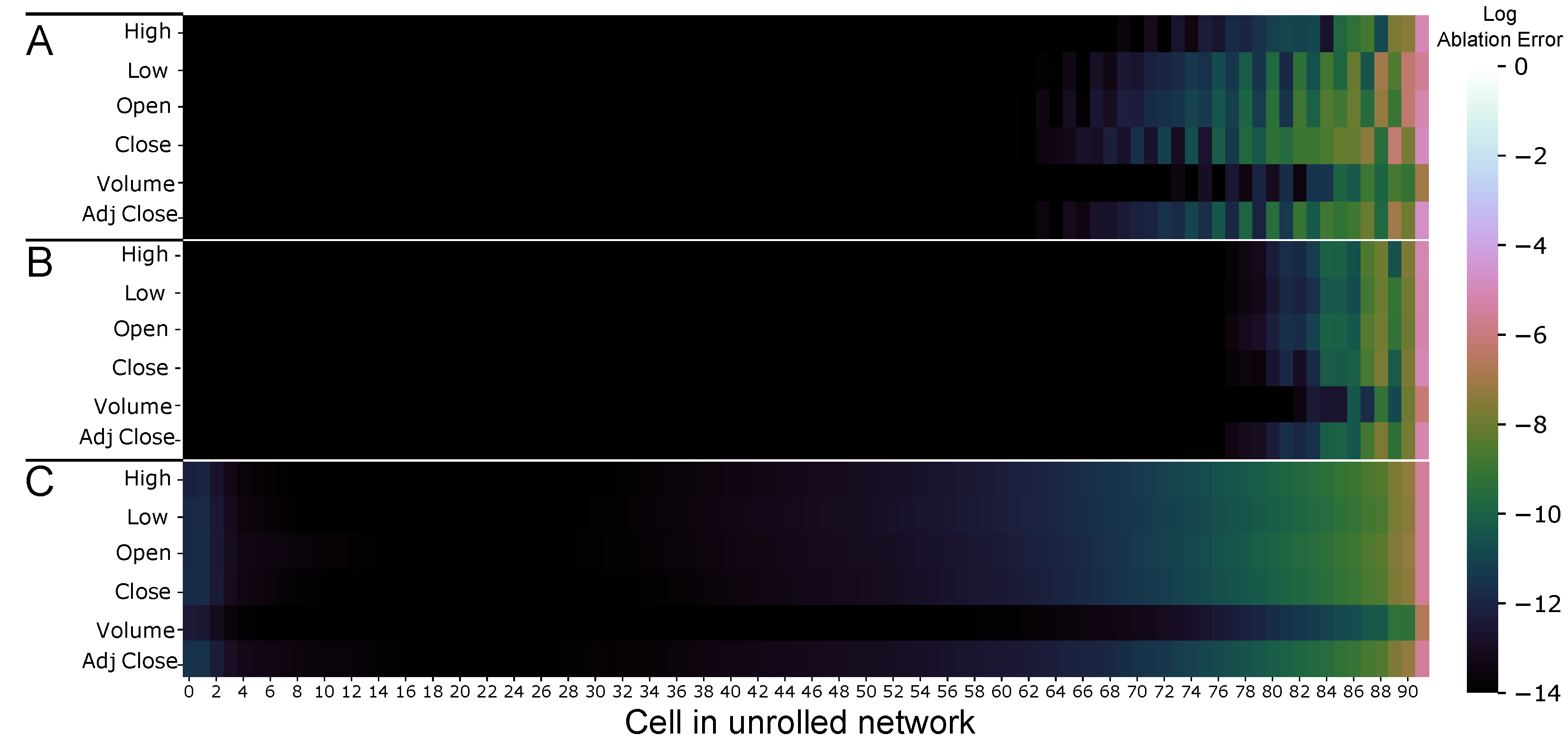
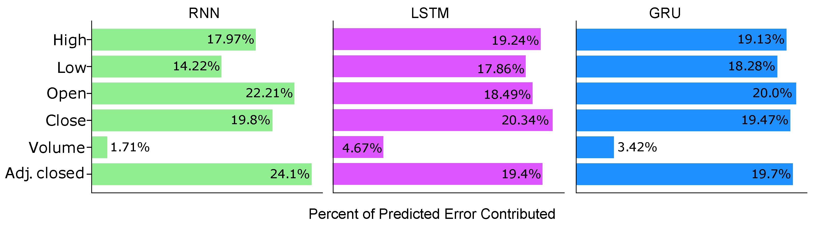
3.1. Ablation

Ablation can be considered a more straightforward form of integrated gradients: the technique removes information from a feature, and the change in prediction is measured. We can then use the magnitude of the predictive error to infer a feature’s importance. If a feature is noninformative to the prediction, ablating it would fail to produce a large change in prediction, leading to a near-zero error. Following feature importance, a unifying feature between models is that the most informative cells lie at the last few inputs (cells 90–92). Feature importance decays, albeit at different rates, moving backwards through the model. Specifically, the GRU network considers the most features in making predictions, with most of the uninformative inputs situated in cells 4–38 as seen in Figure 4. In contrast, the LSTM shows the least number of informative features, which most are present from the 78th cell. Interestingly, the RNN presents with an alternating banding pattern of features importance from the 60th cell onward. Notably, volume was the only feature that showed the smallest change following ablation in all three models.

3.2. Integrated Gradients

Integrated gradients have become a popular and intuitive method to measure the correlations between the input features and correct prediction. The magnitude of the attribution pertains to how strongly the input correlates to the prediction. In contrast, the sign relates to whether the correlation is positive or negative. A value close to 0 represents a feature with close to no influence on the prediction. In contrast, a high positive value would suggest that the input feature is positively associated with the correct prediction. However, in regression, the signs of the attributes represent regions within the neural networks responsible for increasing (+) or decreasing (−) the prediction, whilst the magnitude refers to the scale of change.

There were both commonalities between the models as well as model-specific features. Notably, the magnitude of the attributions for volume was consistently lower than the attributions for any other feature in a given day, shown in Figure 5. In addition, all three models demonstrated their largest magnitudes clustered towards the last inputs. Interestingly, the patterns of negative attributions presented differently in each model. The RNN model demonstrated an alternating pattern between positive and negative attributions, reminiscent of the banding pattern seen in Figure 4 and Figure 6. This result is contrasted against the LSTM, which had negative attributions localised at the front and the GRU, with negative attributions in the back half (0–40). Furthermore, the LSTM displayed fewer negative attributions than the RNN and the GRU. Lastly, it should be noted that the overall magnitudes found in the GRU model were higher than both the RNN and LSTM, particularly at the early inputs (cells 0–46).

3.3. Added Noise

To determine which cells, and by extension which days were most important to the prediction, a defined level of noise (1%) was added to all inputs in a particular cell. Complementing the ablation results, it is further evidence that almost all the predictive power lies in the last three (90–92) cells, as seen in Figure 6. Furthermore, the decay of importance between models is more clearly visible, where the LSTM shows the most significant decay in importance whilst GRU shows the slowest change. However, it is interesting to note that the same banding pattern present in the RNN ablation results in Figure 4 is also present in Figure 6. Notably, the LSTM shows a banding pattern, but to a lesser extent, between the 87–91th cells. Interestingly, the GRU is the only three to demonstrate a recovery in the magnitude of the error at cells 0–3.

3.4. Permutation

The focus of the permutation methods was to determine which feature contributes the most to the prediction for each RNN architecture. Interestingly, all three models assigned the lowest priority to the volume of traded stock, whilst there was no single feature with the highest priority between the three models, as shown in Figure 7. In addition, there was considerable similarity between feature importance between both GRU and LSTM networks, suggesting that their optimal predictions require each to consider the remaining four features equally. However, this is not unexpected considering that the normalised data for these four features show slight variations. In contrast, the RNN showed the most differences in where it placed importance in its features. The RNN appeared to emphasise the adjusted closing price and the opening rather than the high and low price for stocks.

4. Discussion

4.1. Input Importance

Feature importance provides information to model users on where the learned model focuses when making a prediction. The ablation and integrated gradients methods share this function but perform this differently, leading to complementary results (Figure 4 and Figure 5). However, a notable difference is that the integrated gradients method provides a greater sensitivity than the ablation method since all inputs are assigned an attribution, and the sign provides additional information. Despite deriving more information from attributions, it is notable that the results derived from the ablation method are less abstract. Indeed, the results from the ablations represent the log percentage change in the SMAPE error following ablation of an input, providing tangible understanding to the results. For instance, the black regions in the ablation results are absent in the integrated gradients method, showing practically where the regions of nonimportance lie in the input. Notably, the choice of the baseline is vital as this will considerably alter the results for the integrated gradients method. Subsequently, this discussion considers the baseline whilst interpreting the attributions. Given that XAI forecasting is an emerging field, it is uncertain if there is a better alternative to the baseline used in this study. The conclusions derived from the integrated gradients method are made cautiously and relative to the baseline.

The RNN demonstrated the most irregularity of the results regarding input importance compared to the LSTM and GRU (Figure 4 and Figure 5A). Notably, these irregularities presented as alternating bands of low and high importance. This banding pattern was prevalent in both the magnitudes and signs of the attributions. By considering both the model properties and understanding behind attributions, these results suggest that the function of this pattern is to fine-tune the prediction. The RNN derives most of its meaning from the last three days of input (cells 90–92), whereby all subsequent inputs alternate between adjusting the prediction up and down from the moving average, whilst these adjustments decay in magnitude. This banding pattern is also present in the permuted results (Figure 6). This behaviour suggests that the RNN is randomly adjusting predictions rather than applying focus to specific areas in the data, thus supporting the paradigm that RNNs are unable to learn long-term information. Given this information, the results suggested that the RNN model could provide comparable performance with a smaller input size.

The LSTM architecture has successfully demonstrated its ability to learn long-term patterns in data [41]. Despite this, the LSTM network in this study assigns very little importance to data preceding the 78th cell. There are a few possibilities that could explain this. It may signal a lack of memory from the system, or it may reveal that the model is deliberately forgetting long-term information in order to improve the prediction. The LSTM ablation errors show similarities with those of both the GRU and RNN. Similar to the RNN, the LSTM displays a considerable noise surrounding the most recent inputs but lacks a distinctive banding pattern. Furthermore, the LSTM network demonstrates the spectrum decay of importance present in the GRU network, particularly between the 76–84th day. This decay suggests that this LSTM model displays the ability to learn, as this decay signals the network is retaining past information through the transduction of the cell state through the network. However, the LSTM long-term memory retention appears to be less critical in prediction than in the GRU.

A possible reason is that the sequence length (92) may be insufficient for the LSTM to learn long-term patterns adequately. Given that the LSTM performs better with longer and more complex sequences, the LSTM may rely more on its granularity in remembering information when provided a smaller input size [42]. Unlike the GRU, the LSTM can fine-tune the contents of its memory through the output gate, meaning that the predictive strength of the LSTM, in this context, is derived from how it applies importance explicitly to each input rather than long-term patterns. This idea is further supported when considering the attributions of the LSTM (Figure 5). The LSTM demonstrates the least number of negative attributions, and they are all localised towards the end of the network meaning these inputs are critical in reducing the magnitude of the prediction whilst considering relatively few inputs. Consequently, the LSTM is considering fewer data points of relatively high importance to adjust the prediction down to the correct level. Interestingly, while the 92nd cell confers most of the information to the prediction, it also is the cell that contains most of the negative attributions, excluding the open feature. This result implies that the LSTM functions by primarily considering the opening price, at the 92nd cell, to raise the prediction whilst considering the remaining features to create an upper ceiling to the prediction.

The GRU, much like the LSTM, displays the ability to learn long-term patterns; however, it displays a more simplified architecture [43]. Notably, the GRU in this study demonstrates evidence of learning long-term patterns as it displays consistently higher errors throughout the sequence (Figure 4, Figure 5 and Figure 6). Further supporting the notion of memory in GRUs, the results demonstrate that the GRU uniquely places greater attention on early network inputs. Given that GRUs combine the input and forget gate, creating the update gate, GRUs are only able to act on the entire contents of their memory when remembering past information [43]. Subsequently, GRUs demonstrate less precision in forgetting past information compared to LSTM. Therefore, the results suggest the GRU model relies on remembering more past information while the LSTM leverages its precision in forgetting past information to achieve comparable levels of accuracy. Interestingly, the GRU assigns increased importance to the early cells (0–2), suggesting the use of attention in the GRU in making predictions. This attention shows that the GRU has learned that the start of a financial quarter confers mores information to the future prediction than what occurs during the middle portion. Furthermore, when considering the signs of the attributions, it is clear that most of the attributions increase the prediction, with an initial few inputs serving to lower the prediction (Figure 5C). The positioning and magnitudes of negative attributions suggest that the initial inputs, where the GRU places attention, serve as a fine-tuning mechanism. In contrast, the LSTM remembers less information while considering a few high importance features to modulate prediction. Interestingly, the magnitudes of the first and last attributions in the region of negative attribution are smaller than those in the centre. This observation suggests that the GRU specifies the regions that reduce prediction when the magnitude of the attribution drops below a specific threshold.

4.2. Feature Importance

The results show that the volume of traded stocks had little to no effect in the predictions of all three of the models (Figure 7). The potential reason is that volume only refers to the number of stocks traded within a given day, not necessarily the price. The volume for a given stock could increase following a spike in stock price, indicating investors’ interest in buying the stock. Equally, the volume may also increase following the decrease of a stock, which indicates that investors are selling a given stock following the reduction in stock price. Consequently, volume taken in isolation does not provide a strong correlation to the price of a stock at closing.

Notably, all three models are cognisant of the lack of correlation between volume and closing stock price and have primarily disregarded volume when making predictions (Figure 7). The GRU and the LSTM place higher importance on volume compared to the RNN, and by considering the attributions, the reason becomes clear (Figure 5). In the LSTM, volume importance comes from the negative attributions, whereby 45% of negative attributions fall in the volume feature. In comparison, the GRU focuses on the first few cells (0–4), which contain a region of negative attributions present in the volume feature. While the LSTM uses the most recent inputs to create the upper predictive ceiling, the GRU uses the most distant inputs, where it places attention for its predictive ceiling. This observation around attributions and attention may explain why the RNN largely disregards the volume data: it cannot apply attention in long-term patterns or precisely regulate information retention. Overall, there are striking similarities between the feature importance for the GRU and LSTM compared to the RNN. This similarity is present despite the attributions displaying considerably different modes of prediction (Figure 5). It is unlikely that the ability to retain long-term information, as seen with LSTM and GRU neural networks, is responsible given that the RNN shows greater retention than the LSTM (Figure 4 and Figure 6). Instead, it is more likely that both models lay within the same local minima following training using the same deterministic seed.

5. Conclusions

The overarching goal of this research was to determine if existing XAI methods were transferable to financial time series prediction models. All four presented methods provided complementary results despite testing different aspects of the network, providing a robust means in understanding how each of the three models came about their prediction. Collectively, these results provided insight behind where models place importance on input features and revealed contrasting strategies of prediction fine-tuning between architectures. These results suggest that the principles that form the basis of the explainability methods are applicable in financial time series forecasting and can provide an understanding of their complex architectures. An important limitation of this study is that the methods applied here were not tested on a comprehensive set of architectures, opting for the three standard RNN models instead. The performance of these methods may not apply to all deep learning strategies, as it relies on visualisation to derive meaning. A further limitation is that the methods may not be a suitable fit for CNNs, which are on occasion employed in the finance sector [44,45]. Furthermore, whilst the different error metrics provided an understanding for different aspects of the network, they may not prove intuitive to the average person seeking to benefit from explainable AI. Given these limitations, the recommendation is that future studies should expand to see if such methods apply in deep forecasting strategies and other popular architectures such as CNN. A further recommendation is the development of less abstract metrics to impart more practical information regarding model mechanisms.

References

- Tjoa, E.; Guan, C. A survey on explainable artificial intelligence (xai): Toward medical xai. IEEE Trans. Neural Netw. Learn. Syst. 2020, 32, 4793–4813. [Google Scholar] [CrossRef] [PubMed]
- Rudin, C. Algorithms for interpretable machine learning. In Proceedings of the 20th ACM SIGKDD International Conference on Knowledge Discovery and Data Mining, New York, NY, USA, 24–27 August 2014; p. 1519. [Google Scholar]
- van Zyl, T.L. Machine Learning on Geospatial Big Data. In Big Data: Techniques and Technologies in Geoinformatics; CRC Press: Boca Raton, FL, USA, 2014; p. 133. [Google Scholar]
- Angelov, P.P.; Soares, E.A.; Jiang, R.; Arnold, N.I.; Atkinson, P.M. Explainable artificial intelligence: An analytical review. Wiley Interdiscip. Rev. Data Min. Knowl. Discov. 2021, 11, e1424. [Google Scholar] [CrossRef]
- Parikh, R.B.; Teeple, S.; Navathe, A.S. Addressing bias in artificial intelligence in health care. JAMA 2019, 322, 2377–2378. [Google Scholar] [CrossRef] [PubMed]
- Caruana, R.; Lou, Y.; Gehrke, J.; Koch, P.; Sturm, M.; Elhadad, N. Intelligible models for healthcare: Predicting pneumonia risk and hospital 30-day readmission. In Proceedings of the 21th ACM SIGKDD International Conference on Knowledge Discovery and Data Mining, Sydney, NSW, Australia, 10–13 August 2015; pp. 1721–1730. [Google Scholar]
- Goodman, B.; Flaxman, S. European Union regulations on algorithmic decision-making and a “right to explanation”. AI Mag. 2017, 38, 50–57. [Google Scholar] [CrossRef] [Green Version]
- Bach, S.; Binder, A.; Montavon, G.; Klauschen, F.; Müller, K.R.; Samek, W. On pixel-wise explanations for non-linear classifier decisions by layer-wise relevance propagation. PLoS ONE 2015, 10, e0130140. [Google Scholar] [CrossRef] [PubMed] [Green Version]
- Dieber, J.; Kirrane, S. Why model why? Assessing the strengths and limitations of LIME. arXiv 2020, arXiv:2012.00093. [Google Scholar]
- Lundberg, S.M.; Lee, S.I. A unified approach to interpreting model predictions. In Proceedings of the 31st International Conference on Neural Information Processing Systems, Long Beach, CA, USA, 4–9 December 2017; pp. 4768–4777. [Google Scholar]
- Riberio, M.T.; Singh, S.; Guestrin, C. Why Should I Trust You? Explaining the Predictions of Any Classifier. In Proceedings of the 22nd ACM SIGKDD International Conference on Knowledge Discovery and Data Mining, San Francisco, CA, USA, 13–17 August 2016. [Google Scholar]
- Confalonieri, R.; Coba, L.; Wagner, B.; Besold, T.R. A historical perspective of explainable Artificial Intelligence. Wiley Interdiscip. Rev. Data Min. Knowl. Discov. 2021, 11, e1391. [Google Scholar] [CrossRef]
- Fauvel, K.; Lin, T.; Masson, V.; Fromont, É.; Termier, A. XCM: An Explainable Convolutional Neural Network for Multivariate Time Series Classification. Mathematics 2021, 9, 3137. [Google Scholar] [CrossRef]
- Selvaraju, R.R.; Cogswell, M.; Das, A.; Vedantam, R.; Parikh, D.; Batra, D. Grad-cam: Visual explanations from deep networks via gradient-based localization. In Proceedings of the IEEE International Conference on Computer Vision, Venice, Italy, 22–29 October 2017; pp. 618–626. [Google Scholar]
- Viton, F.; Elbattah, M.; Guérin, J.L.; Dequen, G. Heatmaps for Visual Explainability of CNN-Based Predictions for Multivariate Time Series with Application to Healthcare. In Proceedings of the 2020 IEEE International Conference on Healthcare Informatics (ICHI), Oldenburg, Germany, 30 November–3 December 2020; pp. 1–8. [Google Scholar]
- Meyes, R.; Lu, M.; de Puiseau, C.W.; Meisen, T. Ablation studies in artificial neural networks. arXiv 2019, arXiv:1901.08644. [Google Scholar]
- Covert, I.; Lundberg, S.; Lee, S.I. Understanding global feature contributions with additive importance measures. arXiv 2020, arXiv:2004.00668. [Google Scholar]
- Sundararajan, M.; Taly, A.; Yan, Q. Axiomatic attribution for deep networks. In Proceedings of the International Conference on Machine Learning, Sydney, NSW, Australia, 6–11 August 2017; pp. 3319–3328. [Google Scholar]
- Kopitar, L.; Cilar, L.; Kocbek, P.; Stiglic, G. Local vs. Global Interpretability of Machine Learning Models in Type 2 Diabetes Mellitus Screening. In Artificial Intelligence in Medicine: Knowledge Representation and Transparent and Explainable Systems; Springer: Berlin/Heidelberg, Germany, 2019; pp. 108–119. [Google Scholar]
- Kenny, E.M.; Delaney, E.D.; Greene, D.; Keane, M.T. Post-hoc explanation options for XAI in deep learning: The Insight centre for data analytics perspective. In Proceedings of the International Conference on Pattern Recognition, Virtual Event, 10–15 January 2021; Springer: Berlin/Heidelberg, Germany, 2021; pp. 20–34. [Google Scholar]
- Hyndman, R.J.; Koehler, A.B.; Snyder, R.D.; Grose, S. A state space framework for automatic forecasting using exponential smoothing methods. Int. J. Forecast. 2002, 18, 439–454. [Google Scholar] [CrossRef] [Green Version]
- Hyndman, R.J.; Khandakar, Y. Automatic time series forecasting: The forecast package for R. J. Stat. Softw. 2008, 27, 1–22. [Google Scholar] [CrossRef] [Green Version]
- Nguyen, T.T.; Le Nguyen, T.; Ifrim, G. A Model-Agnostic Approach to Quantifying the Informativeness of Explanation Methods for Time Series Classification. In Lecture Notes in Computer Science, Proceedings of the International Workshop on Advanced Analytics and Learning on Temporal Data, Ghent, Belgium, 18 September 2020; Springer: Cham, Switzerland, 2020; pp. 77–94. [Google Scholar]
- Delaney, E.; Greene, D.; Keane, M.T. Instance-based counterfactual explanations for time series classification. In Lecture Notes in Computer Science, Proceedings of the International Conference on Case-Based Reasoning, Salamanca, Spain, 13–16 September 2021; Springer: Cham, Switzerland, 2021; pp. 32–47. [Google Scholar]
- Bailey, D.H.; Borwein, J.; Lopez de Prado, M.; Salehipour, A.; Zhu, Q.J. Backtest overfitting in financial markets. Automated Trader 2016, 1–8. Available online: https://www.davidhbailey.com/dhbpapers/overfit-tools-at.pdf (accessed on 10 December 2021).
- Sezer, O.B.; Gudelek, M.U.; Ozbayoglu, A.M. Financial time series forecasting with deep learning: A systematic literature review: 2005–2019. Appl. Soft Comput. 2020, 90, 106181. [Google Scholar] [CrossRef] [Green Version]
- Laher, S.; Paskaramoorthy, A.; Van Zyl, T.L. Deep Learning for Financial Time Series Forecast Fusion and Optimal Portfolio Rebalancing. In Proceedings of the 2021 IEEE 24th International Conference on Information Fusion (FUSION), Sun City, South Africa, 1–4 November 2021; pp. 1–8. [Google Scholar]
- Makridakis, S.; Spiliotis, E.; Assimakopoulos, V. The M4 Competition: 100,000 time series and 61 forecasting methods. Int. J. Forecast. 2020, 36, 54–74. [Google Scholar] [CrossRef]
- Mathonsi, T.; van Zyl, T.L. Prediction Interval Construction for Multivariate Point Forecasts Using Deep Learning. In Proceedings of the 2020 7th International Conference on Soft Computing & Machine Intelligence (ISCMI), Stockholm, Sweden, 14–15 November 2020; pp. 88–95. [Google Scholar]
- Makridakis, S.; Spiliotis, E.; Assimakopoulos, V. The M5 accuracy competition: Results, findings and conclusions. Int. J. Forecast. 2020, 32, 8026–8037. [Google Scholar] [CrossRef]
- Mathonsi, T.; van Zyl, T.L. A Statistics and Deep Learning Hybrid Method for Multivariate Time Series Forecasting and Mortality Modeling. Forecasting 2022, 4, 1–25. [Google Scholar] [CrossRef]
- Said, S.E.; Dickey, D.A. Testing for unit roots in autoregressive-moving average models of unknown order. Biometrika 1984, 71, 599–607. [Google Scholar] [CrossRef]
- Kingma, D.P.; Ba, J. Adam: A method for stochastic optimization. arXiv 2014, arXiv:1412.6980. [Google Scholar]
- Srivastava, N.; Hinton, G.; Krizhevsky, A.; Sutskever, I.; Salakhutdinov, R. Dropout: A simple way to prevent neural networks from overfitting. J. Mach. Learn. Res. 2014, 15, 1929–1958. [Google Scholar]
- Paszke, A.; Gross, S.; Massa, F.; Lerer, A.; Bradbury, J.; Chanan, G.; Killeen, T.; Lin, Z.; Gimelshein, N.; Antiga, L.; et al. Pytorch: An imperative style, high-performance deep learning library. Adv. Neural Inf. Process. Syst. 2019, 32, 8026–8037. [Google Scholar]
- Seabold, S.; Perktold, J. Statsmodels: Econometric and statistical modeling with python. In Proceedings of the 9th Python in Science Conference, Austin, TX, USA, 28 June–3 July 2010; Volume 57, p. 61. [Google Scholar]
- Virtanen, P.; Gommers, R.; Oliphant, T.E.; Haberland, M.; Reddy, T.; Cournapeau, D.; Burovski, E.; Peterson, P.; Weckesser, W.; Bright, J.; et al. SciPy 1.0: Fundamental algorithms for scientific computing in Python. Nat. Methods 2020, 17, 261–272. [Google Scholar] [CrossRef] [PubMed] [Green Version]
- Kokhlikyan, N.; Miglani, V.; Martin, M.; Wang, E.; Alsallakh, B.; Reynolds, J.; Melnikov, A.; Kliushkina, N.; Araya, C.; Yan, S.; et al. Captum: A unified and generic model interpretability library for pytorch. arXiv 2020, arXiv:2009.07896. [Google Scholar]
- Hunter, J.D. Matplotlib: A 2D graphics environment. Comput. Sci. Eng. 2007, 9, 90–95. [Google Scholar] [CrossRef]
- Waskom, M.L. Seaborn: Statistical data visualization. J. Open Source Softw. 2021, 6, 3021. [Google Scholar] [CrossRef]
- Gers, F.A.; Schmidhuber, E. LSTM recurrent networks learn simple context-free and context-sensitive languages. IEEE Trans. Neural Netw. 2001, 12, 1333–1340. [Google Scholar] [CrossRef] [Green Version]
- Trinh, T.; Dai, A.; Luong, T.; Le, Q. Learning longer-term dependencies in rnns with auxiliary losses. In Proceedings of the International Conference on Machine Learning, Vancouver, BC, Canada, 30 April–3 May 2018; pp. 4965–4974. [Google Scholar]
- Chung, J.; Gulcehre, C.; Cho, K.; Bengio, Y. Empirical evaluation of gated recurrent neural networks on sequence modeling. arXiv 2014, arXiv:1412.3555. [Google Scholar]
- Hoseinzade, E.; Haratizadeh, S. CNNpred: CNN-based stock market prediction using a diverse set of variables. Expert Syst. Appl. 2019, 129, 273–285. [Google Scholar] [CrossRef]
- Livieris, I.E.; Pintelas, E.; Pintelas, P. A CNN–LSTM model for gold price time-series forecasting. Neural Comput. Appl. 2020, 32, 17351–17360. [Google Scholar] [CrossRef]