Review

Time-Lapse Electrical Resistivity Tomography (TL-ERT) for Landslide Monitoring: Recent Advances and Future Directions

Institute of Methodologies for Environmental Analysis, National Research Council of Italy (CNR-IMAA), C.da S.Loja, I-85050 Tito, PZ, Italy
*
Author to whom correspondence should be addressed.
Appl. Sci. 2022, 12(3), 1425; https://doi.org/10.3390/app12031425
Submission received: 15 November 2021 / Revised: 19 January 2022 / Accepted: 27 January 2022 / Published: 28 January 2022
(This article belongs to the Special Issue Advances in Applied Geophysics)

Abstract

:
To date, there is a growing interest for challenging applications of time-lapse electrical resistivity tomography (TL-ERT) in Earth sciences. Tomographic algorithms for resistivity data inversion and innovative technologies for sensor networks have rapidly transformed the TL-ERT method in a powerful tool for the geophysical time-lapse imaging. In this paper, we focus our attention on the application of this method in landslide monitoring. Firstly, an overview of recent methodological advances in TL-ERT data processing and inversion is presented. In a second step, a critical analysis of the main results obtained in different field experiments and lab-scale simulations are discussed. The TL-ERT appears to be a robust and cost-effective method for mapping the water-saturated zones, and for the identification of the groundwater preferential pathways in landslide bodies. Furthermore, it can make a valuable contribution to following time-dependent changes in top-soil moisture, and the spatio-temporal dynamics of wetting fronts during extreme rainfall events. The critical review emphasizes the limits and the advantages of this geophysical method and discloses a way to identify future research activities to improve the use of the TL-ERT method in landslide monitoring.

1. Introduction

Electrical resistivity tomography (ERT) is a robust and well-consolidated method for near-surface geophysics, with a wide spectrum of applications in the geological, engineering and environmental sciences. This geoelectrical method provides 2D and 3D resistivity images of the subsurface; the basic principle is Ohm’s law and the experimental data are the voltage signals produced by the direct electrical currents (f = 0 Hz) injected into the subsoil and filtered by the artificial noise. Technological advances (i.e., multi-channel arrays, innovative sensors) and novel tomographic algorithms for data inversion have rapidly transformed ERT in one of the most popular geophysical methods. Furthermore, the extreme variability of the resistivity parameter (different order of magnitude, from 1–10 Ohm⋅m of clayey materials to 105 Ohm⋅m of granite rocks) makes it possible to use the ERT method in many geological environments [1,2,3,4].
The ERT method can also be applied to study the time-dependent changes of the resistivity pattern of the subsoil: we used the analysis of 2D and 3D static resistivity images of the subsurface to the process the time-series of resistivity images (time-lapse approach or 4D tomography). The first laboratory and experimental works on time-lapse electrical resistivity tomography (TL-ERT or 4D-ERT) method date back to the period 1995–2005, when they were mainly devoted to monitor the injection of salt water in soil and aquifers [5,6,7,8]. The results of these controlled experiments stimulated the study of the complex relationship between resistivity values and hydraulic parameters.
Since these pioneering activities and seminal papers, the attention of the scientific community to the TL-ERT method has increased considerably, with exponential behavior in the yearly number of articles published in top-leading journals. In the last 20 years, more than 200 papers have been published on ISI journals (Figure 1).
The TL-ERT method found an impressive number of applications crossing different disciplines, from hydrogeology [9,10,11,12] to agriculture [13,14,15,16], from engineering geology [17,18,19,20] to geohazards [21,22,23,24], from CO2 storage [25] to the study of the effects of the climate changes on soil and near subsurface [26,27,28,29].
Here, we focus our attention on the application of the TL-ERT method for landslide monitoring. In the last years, climate change and the occurrence of frequent extreme meteorological events have contributed to the triggering of landslide phenomena, with considerable effects on the economic and social life of the affected areas [30,31,32]. Indeed, the number of cases in which these phenomena involved strategic infrastructures (e.g., bridges, railways, highways) as well as civil housing and commercial activities [33,34,35], sometime causing fatalities [36,37], has considerably grown.
Taking this into account, the need to develop early warning systems allowing officials to monitor the variation of specific subsoil parameters responsible for triggering landslides has become more pressing [38,39,40]. Alongside the more classic monitoring systems, based on the use of purely geotechnical sensors, such as inclinometers, piezometers, etc., innovative systems based on indirect measures such as geophysical ones [41] have begun to be experimented with. Geophysical methods allow the measure of physical parameters, whose variation often depends on the variation of parameters directly related to the triggering of landslides (for example the water content, the porosity of the rock, etc.). The ERT method can be considered one of the most widely applied geophysical methods in the study of landslides. Many examples of 2D and 3D ERT applications (Figure 2) for the geometric characterization of the landslide body, the identification of the sliding surface, and the localization of areas with higher water content, are reported in the literature [42,43,44].
Recent technological improvements, which have allowed acquisition time to speed up in order to obtain many measurements and develop innovative algorithms for data inversion, have made it possible to test the ERT method and monitor landslides.
Indeed, considering the dependence of the electrical resistivity on the water content and the role that the latter plays in the triggering of landslides, repeated resistivity measurements over time along defined profiles (TL-ERT) can be carried out with the aim of monitoring, for example, the water content variations in the first subsoil levels and to try to define triggering thresholds.
Compared to other fields of application, the use of the TL-ERT in landslide monitoring can be considered recent. The geological complexity of the investigated phenomenon still requires additional experimentations and the development of petrophysical laws that allow quantitative correlation between the electrical resistivity values and the hydrologic parameters directly involved in the triggering of landslides.
In this paper, a selected list of papers extracted by the WOS database for the period 2010 up to now, concerning the TL-ERT method and its application for landslide monitoring, have been considered. The main goals of this work are: (i) to perform an overview of the recent methodological advances in TL-ERT data processing and inversion; (ii) to identify the limits and the advantages of this method when it is applied in monitoring hydrogeological phenomena; (iii) to perform a critical analysis with the identification of future directions for the research activity on this topic.
The work has been organized as follows. In the first step, the basic principles and the algorithms for data inversion of the TL-ERT method are briefly summarized. In a second step, a systematic overview of the main results obtained with this method in a selected list of field-scale experiments for landslide monitoring is carried out. Finally, some gaps and future methodological and technological trends are identified and discussed.

2. The TL-ERT Method: Data Processing and Inversion

2.1. Basic Principles

The TL-ERT method is based on the analysis of a dataset of 2D or 3D resistivity images obtained at different time intervals: it combines 2 or 3 spatial dimensions with a temporal dimension (4D ERT). The TL-ERT or 4D ERT method adopts multi-electrode arrays and the data acquisition procedures already used for the classical 2D and 3D ERT surveys, but the acquisition is generally controlled by a remote system, and it is repeated over time. The main experimental errors associated with the TL-ERT measurements are connected to the presence of man-made electrical noises, galvanic contact changes, electrode corrosion, and low signal-to-noise ratio in voltage signals (well-known sources of errors in 1D, 2D and 3D ERT measurements). The stacking techniques and algorithms for spectral analysis are generally used for extracting the weak voltage signals generated by the current injection into the subsurface, also in the condition of low signal-to-noise ratio [1,4,42]. However, it is necessary to consider other time-related errors connected to temperature and galvanic changes, such as rain precipitation and variations of electrode spacings due to surface ground movements [45].
As it concerns the interpretation and the inversion of the 4D ERT experimental data, the simpler and more common approach is based on the analysis of the differences between the resistivity images independently inverted during the acquisition phase (independent approach). However, the time-lapse of the resistivity images can easily produce an amplification of the inversion artifacts [46].
Another largely applied method is the difference inversion of the ERT data [47]. The Occam algorithm was modified to allow the inversion of the differences between the background or reference resistivity images and the other 3D resistivity images obtained at a different time. The resistivity obtained by the inversion of background data serves as a priori model in the difference inversion. The method allows a rapid convergence of the inversion process and reduces the errors due the field array configurations.
A ratio inversion was proposed by Daily 1992 [48], in which the inversion is performed using the ratio between two successive ERT measurements multiplied with a resistivity value representing a homogenous subsurface model. An alternative approach is the cascaded inversion: this method uses the inversion result of the initial dataset as the starting and reference model for the inversion of the subsequent datasets [49].
Another critical error affecting the interpretation of the TL-ERT data is the assumption of the time-invariant (static) subsurface model during the acquisition phase. This hypothesis is realistic for slow phenomena, but in field experiments we could observe rapid changes of the subsurface model (i.e., the migration of a fluid in a fractured material). To overcome this problem, Kim et al. (2009) [50] introduced a subsurface resistivity model that is continuously changed over the time, the model is completely defined in the space-time domains, and the inversion algorithm considers all data available (Full 4D TL-ERT data inversion). To reduce the computing time and to stabilize the inversion procedure, some regularization criteria are generally introduced.

2.2. Novel Algorithms for Data Processing and Inversion

After these seminal works, the TL-ERT method has found an impressive and large spectrum of applications, and many authors have proposed new methods for TL-ERT data analysis and inversion [4]. In past years, the number of papers on this topic has constantly grown. Here, an overview of selected papers published during the last ten years is presented.
Doetsch et al., 2010 [51], proposed a structural joint inversion using cross-gradient constraints of the time-lapse GPR and ERT data. They analyzed synthetic and experimental data collected during a water injection experiment. The structure is imposed when the updates of the model, with respect to the background, is in the same or opposite directions. Synthetic and experimental tests confirmed the capacity of the structural joint inversion to better describe the plumes geometry, with respect to the single individual inversion.
Herckenrath et al., 2011 [52] investigated the possibility to calibrate the hydrogeophysical inversion with the time domain electromagnetic (TDEM) and ERT data. A geophysical model was simultaneously inverted with a groundwater model by coupling the groundwater and geophysical parameters. Jardani et al., 2013 [53] used a stochastic joint inversion of resistivity and self-potential data integrated with in-situ measurements of hydrogeological parameters. The main results of the inversion revealed that incorporating the self-potential data improves the estimate of hydraulic conductivity.
Camporese et al., 2015 [54] analyzed the performance of coupled and uncoupled inversion approaches in the reconstruction of heterogeneous saturated hydraulic conductivity patterns. The comparison was carried out in the framework of a model inversion based on the ensemble Kalman filter. The results highlighted some advantages of the coupled approach, but it requires massive computational resources.
The joint inversion of geophysical data and the coupled inversion of hydrogeophysical data are extremely complex issues and challenging scientific problems, for this reason, there are not many papers about the joint inversion of the TL-ERT data with other geophysical measurements. Furthermore, there is a growing interest in the studies on hydrogeophysical and petrophysical relationships.
Many works are focused on improving and modifying the full 4D inversion algorithm based on the regularization in space and time [50]. Hayley et al., 2011 [55], introduced the concept of simultaneous inversion. They proposed two different approaches: in the first one, the inversion of two consecutive ERT datasets was performed under a single optimization procedure and constraints, to ensure that the changes from one time to another were smooth; in the second method, the inversions were performed simultaneously and constraints of smoothness and closeness to a reference model were applied to the difference image produced.
Karaoluis et al., 2011 [56] modified the method for the full 4D inversion based on the regularization in space and time. They introduced the concept of the 4D active time-constrained (4D-ATC) inversion. The main feature of the modified algorithm is that it allows the time regularization to vary between different time steps depending on the degree of spatial resistivity changes occurring among different monitoring stages. As a result, the 4D-ATC algorithm uses all the benefits of the 4D algorithm, but also introduces increased flexibility in terms of temporal regularization, which can help in focusing on the dynamic resistivity changes. In a successive work, Karaoluis et al., 2014 [57], proposed an inversion scheme based on distributed and non-uniform parameters, considering the time-related noise and the reduction of the sensitivity in ERT measurements as purely random.
Other improvements were based on the concept of the adaptive approach and the use of minimum gradient in TL-ERT data inversion. Wilkinson et al., 2015 [58] proposed, for the first time, an adaptive survey technique for geoelectrical monitoring. A static algorithm was modified for increasing the resolution within target zones; during the time-dependent period from the image analysis, the zones were interested by the resistivity changes, and the resolution within these zones in the successive ERT acquisition increased. Nguyen et al., 2016 [59] introduced the concept of the minimum gradient support (MGS) in the TL-ERT data inversion. This parameter was selected using the value of the TL-ERT data root mean square misfit and the first iteration of the inversion procedure.
Some recent works are mainly devoted to the development of innovative algorithms for considering and removing the influence of artifacts and errors in the TL-ERT inversion procedure.
Liu et al., 2017 [60] approached the problems related to the propagation of the false anomalies in the initial model and their propagation in the successive TL-ERT inversions, and the assumption of the uniform sensitivity to resistivity variations. They introduced a temporal gradient to enhance the vertical and/or horizontal variation of the model parameters, and normalized the observations before inversion.
Lesparre et al., 2017 [61] analyzed the problems related to the quantification of the errors in the TL-ERT data inversion. Their approach was based on the analysis of the differences between normal and reciprocal measurements (i.e., swapping of the energizing and measuring electrodes) acquired at different time. They extended the concept of the static error formed by a linear combination of the systematic and random components [7], the results emphasized the necessity to better evaluate the errors in the time-lapse resistivity monitoring independently by the algorithm inversion.
Tso et al., 2017 [62] organized an overview of the main methodologies for removing and minimizing the influence of the experimental errors in the ERT inversion algorithms. They extended the standard error model based on the linearity with the transfer resistance introducing a grouping variable based on the electrode number used for the experimental measurements. This new linear mixed model (LME) was tested using lab and field data, improving the quality of the ERT images.
Other works focus their attention on errors due to the presence of an irregular surface topography in the area interested by the field measurements [17], and the acquisition schemes with electrodes installed in the boreholes [63].
Furthermore, there are some studies based on the use of the classical Kalman Filter, Bayesian Markov chain, Monte Carlo simulation and clustering procedures for the TL-ERT data analysis and inversion. Notwithstanding these methods are largely applied in geophysics, there is a limited number of applications on the time-dependent geoelectrical monitoring. Saibaba et al., 2014 [64], introduced the Kalman filtering approach to analyze the TL-ERT data. This model is useful in practical applications in which data is acquired at a rapid rate, and when changes in subsequent states are small and can be approximated by a random process.
Oware et al., 2019 [65] developed a novel method for the TL-ERT data inversion using a Bayesian Markov chain Monte Carlo (McMC) technique. The approach was based on the parametrization of the Bayesain inversion model in terms of the optimal bases, which allows a sparse representation of the desired features leading to dimensionality reduction and Monte Carlo simulations tuned to the physics of the targeted process. The method was tested during a heat-tracer experiment. Delforge et al., 2021 [66] proposed the time clustering method as a tool for the post-inversion of the TL-ERT data. The authors tested three different algorithms (K-means, hierarchical agglomerative clustering, and Gaussian Mixture Model) on raw ERT data analyzing the role of the spatial constraints and evaluating the robustness of the method.
Recently, there has been growing attention on the development of open sources software and codes, and the use of parallel computing to reduce the time required for geophysical data inversion. As it concerns the TL-ERT data, Johnson et al., 2017 [67] used open-source codes to simulate spatio-temporal changes of subsurface resistivity. The module PFLOTRAN-E4D operating in parallel modality was applied to reconstruct the bulk electrical conductivity from a subsurface flow and transport simulation code. At each step of the iterative process, a tomographic image is simulated using the bulk electrical conductivity model. This multi-physics approach appears of great interest for the availability of open-source codes.
Rucker et al., 2017 [68] introduced an open-source framework for the inversion of a hydro-geophysical dataset. A pyGIMLi (Python Library for Inversion and Modelling in Geophysics) was implemented for solving the minimization problem with a Gauss–Newton algorithm for any forward operator. The method was used for incorporating hydrological and petrophysical constraints in the ERT data inversion. Blanchy et al., 2020 [69] introduced the open-source code RESIPy for the inversion of resistivity and induced polarization data. The code can also be used for the analysis of TL-ERT data. It is formed by three different layers: (i) the first one is composed of inversion codes R2, R3t and CR2 and a software to generate triangular meshes; (ii) the second layer is composed of Python API, containing processing routines for filtering and error modeling; (iii) the last is composed of routines for graphical application mainly devoted to data visualization.
Liu et al., 2020 [70] proposed a method for the fast inversion of the 4D ERT data that considers the problems related to the rapid changes in the resistivity subsurface model. Generally, the ERT inversion is time consuming, and during the period necessary for the data inversion a resistivity change in the subsurface could occur. The algorithm subdivided an entire data set into a multiple subset of data, that were dynamically substituted in the equations for data inversion. In this process, the regularization coefficients are adjusted; furthermore, a GPU parallel algorithm is used for the TL-ERT data inversion.
Finally, in Table 1 we summarize the different methods adopted for TL-ERT data inversion. At each class is associated a list of the selected works previously discussed. Of course, the list is not exhaustive, and does not include all of the published papers.

3. Landslide Monitoring

Landslide investigation is one of the more consolidated applications of the ERT method. The main contributions of the static 2D and 3D ERT (Figure 2) tomographic methods regard the delineation of the geometry of the landslide bodies and the identification of high water content areas [42,44,71]. As it concerns the landslide monitoring, the TL-ERT method represents an optimal tool to investigate the triggering factors of mass-movements related to water infiltration, and soil moisture’s temporal and spatial changes. In fact, the time series of the resistivity images are strongly influenced by the time-dependent changes of water content in soil and subsoil.
Lebourg et al., 2010 [72] performed a field experiment at the Vence landslide (France), considered as a translational landslide, including 1.2 × 10⁶ m3 of material. They measured rainfall precipitation for three months, including water level and resistivity values, and investigated the possible correlations between these parameters. The study was carried out using raw data (apparent resistivity values) without any inversion, the results pointed out the strong negative correlations between the rainfall events and the resistivity correlation factor, and between the piezometric elevation and the resistivity average.
Travelletti et al., 2012 [73] carried out another field experiment at the Laval landslide (France). Starting from a non-saturated condition near the surface, the TL-ERT measurements were performed during water infiltration within clay-shale material. They observed a reduction of resistivity values (18%) with an asymptotic value in correspondence to steady state flow conditions. The inversion of the TL-ERT data was carried using different methods [2,49], and the results highlighted possible preferential flows near the landslide toe in the steady stationary flow (Figure 3). Other field experiments planned for landslide investigations in Taiwan and Italy are reported in Lee et al., 2012, Luongo et al., 2012, and Quagliarini et al., 2017 [74,75,76].
Gunn et al., 2013 [77] investigated the complex geological environment of the Whitby Mudstone Formation, one of the highest landslide densities in the United Kingdom. They studied the landslide phenomena at Hollin Hill in North Yorkshire that includes shallow, retrogressive rotational, and translation movements. A permanent station able to perform time-lapse ERT observations was installed for monitoring the soil moisture pattern near the surface: the results allowed the authors to study the role of hydrogeological processes in triggering earth flows.
Gance et al., 2016 [78] installed a permanent 4D-ERT system at the Super-Sauze clayey landslide (France). They performed a statistical analysis to investigate possible relationships between the rainfall characteristics, the soil hydrological observations and the soil electrical resistivity response (Figure 4). The results highlighted the influence of the temperature in ERT measurements due to the heat exchange between the groundwater, the vadose zone water and the rainwater that hides the variations of resistivity due to variations in the soil water content. Another quite similar experiment was carried out in a landslide area in southwestern China, to map the pathways of rainwater infiltration in the slipping zones (Xu et al., 2016) [79].
Palis et al., 2017 [80] applying electrical resistivity tomography (daily acquisition), rainfall records (since 2006) and boreholes monitoring groundwater level (since 2009), carried out a 9.5-year multiparametric survey on the “Vence” (France) landslide. The aim of the survey was to understand fluid circulations within the unstable slope. ERT data were analyzed by using an automated clustering analysis enabled to isolate the ERT section into three groups of apparent resistivity values (Figure 5). The comparison between the variations of these cluster behaviors in time with the variations of groundwater levels on site, allowed the authors to locate distinct hydrogeological units. The authors showed that the qualitative information on the variability of the slope hydrogeological behavior could help improve the conversion of resistivity data into hydrologic quantities.
Zieher et al., 2017 [81] performed a spray irrigation experiment in a selected Alpine zone interested by shallow landslides. A sequence of 2D ERT images were obtained during the irrigation period. Furthermore, they installed a grid of time-domain reflectometry sensors at different depths for measuring water content, and used a linear diffusion model for simulating the time-dependent variations of the pore pressure. The results allowed them to detect the negative resistivity changes associated with the vertical progressing water. Unfortunately, the measurements and the model were not able to investigate the small-scale variations in pore pressure that may facilitate the triggering of shallow landslides.
Hojat et al., 2019 [82] carried out a laboratory-scale experiment to simulate the rainfall triggering of shallow landslides. They used the TL-ERT and time-domain reflectometry methods to monitor water infiltration and to evaluate the volumetric water content. After a calibration of the Archie’s equation, the ERT images were transformed in water saturated maps. The results of the controlled experiment highlighted that the landslide body becomes unstable at zones where the water saturation exceeds 45%, and the instability phenomena could occur at the boundaries between areas with different water saturations.
Ivanov et al., 2020 [83] approached the study of shallow landslides in a mountain landscape mainly triggered by rainfall extreme events. They designed and implemented a landslide simulator, and a dataset of 20 land mass failures induced by water infiltration were described and analyzed. Both hydrogeological and TL-ERT measurements were performed. The time series of the ERT images were used for mapping the waterfront time-dependent changes during three different rainfall simulations: (i) temporal increase in the rainfall intensity; (ii) constant rainfall intensity and (iii) two sequences for rainfall events. The results of downscaled experiments confirmed that the rainfall intensity, the hydraulic conductivity and the soil moisture gradient controlled the stability, while rainfall intensity and duration were the main predictors of the shallow soil slips. Furthermore, their results could be useful for implementing procedures for the validation of the rainfall thresholds.
Boyd et al., 2021 [84] investigated one of the more critical problems that generally occur in the ERT monitoring of shallow landslides. It is common to observe low changes in the geometry of the electrode array due to ground movements. In a field experiment carried out at Hollin Hill site (UK), the variations of the distances between the electrodes were detected with topographic methods (UAV surveys and global position measurements) and considered in the TL-ERT inversion (Figure 6).

4. Discussion

This review helps to highlight the strengths and weaknesses of the TL-ERT method in the study of landslide areas, by considering both the technological aspects of instrumentation and data acquisition, and the phase of data analysis and processing.
As shown by the papers analyzed in the previous section, the main and robust contributions of the TL-ERT method in the study of landslides concern the monitoring of rainwater infiltration in the shallow subsurface, and the estimation of the spatial and temporal changes in soil moisture and water content in the top soils and shallow layers of the unstable slope, respectively. In many cases, authors tried to define significant correlations between rainfall, soil hydrological characteristics, and resistivity values [72,78,80]. The quantitative analysis of such correlations has always represented a challenge for the scientific community. Very often, the TL-ERT measurements have been integrated and compared with meteorological and hydrological data and, sometimes, with TDR measurements or other geophysical data [81,82]. The comparison and integration of data coming from different techniques allow the overcoming of some specific limitations of each single method. The results of the integration highlight the capability of TL-ERT to give quantitative information about the water content and to map a preferential pathway for water infiltration. This capability makes the TL-ERT method useful in the future for better evaluating the water saturation effects in the estimation of the rainfall thresholds in landslide early-warning systems.
The analyzed papers also confirmed that it is not possible to generalize the results obtained for every geological and geomorphological context. In order to make the landslide monitoring effective by applying the TL-ERT method, an appropriate and correct geological model must be adopted. As reported by other authors, the petrophysical models used to transform resistivity values in hydrological parameters are site-specific [81,85], and cannot be used to define resistivity thresholds applicable for the activation of landslides in any geological environment. The main evolution of the petrophysical relationships reported in the literature has regarded the change of the number of phases to be considered in the model [86]. Indeed, unlike what is claimed by the petrophysics, the rock formations are unconsolidated, and not composed of a continuous solid phase, but of different phases. So, starting from the one phase (pore water) model proposed by Archie’s Law [87], to interpret the electrical properties acquired in different sedimentary contexts, multi-phase models have been considered [88].
Despite the attention paid by the scientific community, the numerous developed petrophysical relationships are still difficult to apply in the study of landslide areas. Often, they require calibration with other parameters (i.e., soil temperature, porosity, water content, etc.) that are not always available or measurable, requiring laboratory analysis for their definition. For this reason, authors working in landslide areas often prefer to consider the raw data and carry out a statistical analysis of them.
All the discussed applications were carried out almost exclusively in rural areas, i.e., in areas where the logistical conditions for data acquisition were favorable, and in which the quality of the data was generally high due to the absence of environmental noise sources. Working in rural areas offers some advantages, such as easier positioning of the instrumentation and planning of continuous acquisition over time (the electrodes can be embedded in the ground for long periods without creating problems for the normal activities of a community). The absence of buried objects and underground utilities, that could affect the flow of current in the subsoil, and the good electrode/terrain coupling mean that the acquired data are not very noisy, and do not require high filtering actions. Despite these, many authors, to avoid the appearance of the artifacts in the final image, prefer to analyse the apparent resistivity data, instead of applying inversion algorithms.
As described in paragraph two, in the last ten years an impressive number of papers concerning novel algorithms for resistivity data processing and inversion have been published. However, there are a limited number of cases in which these algorithms have been applied to analyze the TL-ERT data measured in field-experiments carried out for studying landslides. Probably, the use of these mathematical methods is quite complicated when applied to experimental data characterized by large variability in spatial and temporal domains, and affected by a high-level of anthropic noise. The TL-ERT data inversion must also consider the effect of the temperature in the first layers of the subsoil and, in active landslides, the effect of the electrode’s movement. Corrective formulas have been introduced for both critical issues [78,84].
A gap between the quality of the algorithms that are currently available for the TL-ERT data inversion and the methods routinely applied in the interpretation of the experimental resistivity data is quite evident. The use of advanced methods for data processing and inversion will disclose the possibility to apply the TL-ERT method in the monitoring of landslides occurred in urban areas and complex geological slopes.
Except for a few studies [80,85], all the acquisitions were carried out along 2D longitudinal profiles. This still represents a limitation of the method, as the investigated object has a 3D structure. Unfortunately, making 3D acquisitions is not easy and requires the use of manageable instruments. Other reviews [4,42] have already highlighted this aspect, referring, as a possible solution, to the use of separate current injections and voltage measuring systems, but also to the experimentation of technologies that minimize the number of cables (smart sensors and web-based services for wireless sensor networks). Considering the difficulties that characterize 3D acquisition in landslide areas, it is well understood that these difficulties increase if we want to realize a 3D time-lapse ERT.
Other weaknesses identified by the critical analysis of the works presented in the previous paragraph concern the TL-ERT’s difficulty in investigating deep subsoil layers in landslide bodies. The ERT method can investigate shallow (0–20 m) and deep layers (>50 m) in landslide bodies, but there are no experimental tests in which the time-lapse monitoring systems have been able to obtain information about the resistivity patterns in deep environments. Generally, the amplitude of the time-dependent changes of resistivity values are higher in shallow layers, and strongly decrease in deep environments; however, the possibility to detect weak perturbations in the resistivity patterns of deep environments (50–100 m) could be very interesting and challenging. In the future, the design of TL-ERT monitoring systems to obtain a time series of 3D resistivity images with an investigation range of 0–100 m could open new research opportunities.

5. Conclusions

Two very significant aspects emerge from the analysis of the papers published in the period 2010–2020 on the theoretical developments and related applications of the TL-ERT method. The first concerns the enormous development of innovative methodologies for the processing and interpretation of data acquired with the TL-ERT method, while the second resides in the wide and growing spectrum of applications of this method in landslide monitoring.
The TL-ERT method appears particularly suitable for studying the variations, both in the spatial and temporal domain, of water content in the most superficial layers of the soil in landslide bodies. It can also provide a useful contribution to the identification of preferential ways for the infiltration of fluids. In the future, this activity could make a significant contribution in early warning systems for landslides induced by extreme weather events by also applying the TL-ERT method to evaluate the water saturation effects in the estimation of the rainfall thresholds.
However, it will be necessary to investigate the complex relationships between resistivity and hydrogeological parameters. From the analysis of the results obtained, the use of innovative mathematical and statistical methods in interpreting the experimental results still appears to be limited. This aspect is fundamental in making the insertion of this method more robust in advanced and widespread monitoring systems. Finally, the TL-ERT method should also be applied for deeper geophysical investigations.

Author Contributions

Conceptualization, V.L. and A.P.; methodology, V.L. and A.P.; writing—original draft preparation, V.L. and A.P.; writing—review and editing, V.L. and A.P. All authors have read and agreed to the published version of the manuscript.

Funding

This research was carried out in the framework of the projects OT4CLIMA “Advanced EO technologies for studying Climate Change impacts on the environment” (D.D. 2261 of 6.9.2018, MUR PON R&I 2014–2020 program) and MITIGO “Mitigazione dei rischi naturali per la sicurezza e la mobilità delle aree montuose del Sud Italia” (ARS01_00964, MUR PON R&I 2014–2020 Program).

Institutional Review Board Statement

Not applicable.

Informed Consent Statement

Not applicable.

Acknowledgments

The authors thank Rocchino Caivano for the technical support in the bibliography classification and organization using the WoS database.

Conflicts of Interest

The authors declare no conflict of interest.

References

  1. Koefoed, O. Geosounding Principles 1: Resistivity Sounding Measurements; Elsevier: Amsterdam, The Netherlands, 1979. [Google Scholar]
  2. Loke, M.H.; Barker, R.D. Rapid least-squares inversion of apparent resistivity pseudosections using a quasi-Newton method. Geophys. Prospect. 1996, 44, 131–152. [Google Scholar] [CrossRef]
  3. Loke, M.H.; Barker, R.D. Practical techniques for 3D resistivity surveys and data inversion. Geophys. Prospect. 1996, 44, 499–523. [Google Scholar] [CrossRef]
  4. Loke, M.H.; Chambers, J.E.; Rucker, D.F.; Kuras, O.; Wilkinson, P.B. Recent developments in the direct-current geoelectrical imaging method. J. Appl. Geophys. 2013, 95, 135–156. [Google Scholar] [CrossRef]
  5. Binley, A.; Henry-Poulter, S.; Shaw, B. Examination of solute transport in an undisturbed soil column using electrical resistance tomography. Water Resour. Res. 1996, 32, 763–769. [Google Scholar] [CrossRef]
  6. Slater, L.; Binley, A.; Brown, D. Electrical imaging of fractures using groundwater salinity change. Ground Water 1997, 35, 436–442. [Google Scholar] [CrossRef]
  7. Slater, L.; Binley, A.; Versteeg, R.; Cassiani, G.; Birken, R.; Sandberg, S. A 3D ERT study of solute transport in a large experimental tank. J. Appl. Geophys. 2002, 49, 211–229. [Google Scholar] [CrossRef]
  8. Kemna, A.; Vanderborght, J.; Kulessa, B.; Vereecken, H. Imaging and characterisation of subsurface solute transport using electrical resistivity tomography (ERT) and equivalent transport models. J. Hydrol. 2002, 267, 125–146. [Google Scholar] [CrossRef]
  9. Earon, R.; Riml, J.; Wu, L.W.; Olofsson, B. Insight into the influence of local streambed heterogeneity on hyporheic-zone flow characteristics. Hydrogeol. J. 2020, 28, 2697–2712. [Google Scholar] [CrossRef]
  10. Paz, M.C.; Alcala, F.J.; Medeiros, A.; Martinez-Pagan, P.; Perez-Cuevas, J.; Ribeiro, L. Integrated MASW and ERT Imaging for Geological Definition of an Unconfined Alluvial Aquifer Sustaining a Coastal Groundwater-Dependent Ecosystem in Southwest Portugal. Appl. Sci. 2020, 10, 5905. [Google Scholar] [CrossRef]
  11. Folch, A.; del Val, L.; Luquot, L.; Martinez-Perez, L.; Bellmunt, F.; Le Lay, H.; Rodellas, V.; Ferrer, N.; Palacios, A.; Fernandez, S.; et al. Combining fiber optic DTS, cross-hole ERT and time-lapse induction logging to characterize and monitor a coastal aquifer. J. Hydrol. 2020, 588, 125050. [Google Scholar] [CrossRef]
  12. Palacios, A.; Ledo, J.J.; Linde, N.; Luquot, L.; Bellmunt, F.; Folch, A.; Marcuello, A.; Queralt, P.; Pezard, P.A.; Martinez, L.; et al. Time-lapse cross-hole electrical resistivity tomography (CHERT) for monitoring seawater intrusion dynamics in a Mediterranean aquifer. Hydrol. Earth Syst. Sci. 2020, 24, 2121–2139. [Google Scholar] [CrossRef]
  13. Rao, S.; Lesparre, N.; Orozco, A.F.; Wagner, F.; Javaux, M. Imaging plant responses to water deficit using electrical resistivity tomography. Plant Soil 2020, 454, 261–281. [Google Scholar] [CrossRef]
  14. Fishkis, O.; Noell, U.; Diehl, L.; Jaquemotte, J.; Lamparter, A.; Stange, C.F.; Burke, V.; Koeniger, P.; Stadler, S. Multitracer irrigation experiments for assessing the relevance of preferential flow for non-sorbing solute transport in agricultural soil. Geoderma 2020, 371, 114386. [Google Scholar] [CrossRef]
  15. De Carlo, L.; Battilani, A.; Solimando, D.; Caputo, M.C. Application of time-lapse ERT to determine the impact of using brackish wastewater for maize irrigation. J. Hydrol. 2020, 582, 124465. [Google Scholar] [CrossRef]
  16. Blanchy, G.; Watts, C.W.; Richards, J.; Bussell, J.; Huntenburg, K.; Sparkes, D.L.; Stalham, M.; Hawkesford, M.J.; Whalley, W.R.; Binley, A. Time-lapse geophysical assessment of agricultural practices on soil moisture dynamics. Vadose Zone J. 2020, 19, e20080. [Google Scholar] [CrossRef]
  17. Bievre, G.; Oxarango, L.; Gunther, T.; Goutaland, D.; Massardi, M. Improvement of 2D ERT measurements conducted along a small earth-filled dyke using 3D topographic data and 3D computation of geometric factors. J. Appl. Geophys. 2018, 153, 100–112. [Google Scholar] [CrossRef]
  18. Jodry, C.; Lopes, S.P.; Fargier, Y.; Sanchez, M.; Cote, P. 2D-ERT monitoring of soil moisture seasonal behaviour in a river levee: A case study. J. Appl. Geophys. 2019, 167, 140–151. [Google Scholar] [CrossRef] [Green Version]
  19. Masi, M.; Ferdos, F.; Losito, G.; Solari, L. Monitoring of internal erosion processes by time-lapse electrical resistivity tomography. J. Hydrol. 2020, 589, 125340. [Google Scholar] [CrossRef]
  20. Srivastava, S.; Pal, S.K.; Kumar, R. A time-lapse study using self-potential and electrical resistivity tomography methods for mapping of old mine working across railway-tracks in a part of Raniganj coalfield, India. Environ. Earth Sci. 2020, 79, 332. [Google Scholar] [CrossRef]
  21. Di Giuseppe, M.G.; Troiano, A. Monitoring active fumaroles through time-lapse electrical resistivity tomograms: An application to the Pisciarelli fumarolic field (Campi Flegrei, Italy). J. Volcanol. Geotherm. Res. 2019, 375, 32–42. [Google Scholar] [CrossRef]
  22. Tso, C.H.M.; Johnson, T.C.; Song, X.H.; Chen, X.Y.; Kuras, O.; Wilkinson, P.; Uhlemann, S.; Chambers, J.; Binley, A. Integrated hydrogeophysical modelling and data assimilation for geoelectrical leak detection. J. Contam. Hydrol. 2020, 234, 103679. [Google Scholar] [CrossRef] [PubMed]
  23. Peskett, L.; MacDonald, A.; Heal, K.; McDonnell, J.; Chambers, J.; Uhlemann, S.; Upton, K.; Black, A. The impact of across-slope forest strips on hillslope subsurface hydrological dynamics. J. Hydrol. 2020, 581, 124427. [Google Scholar] [CrossRef]
  24. Bouvier, C.; Adamovic, M.; Ayral, P.A.; Brunet, P.; Didon-Lescot, J.F.; Domergue, J.M.; Spinelli, R. Characterization of subsurface fluxes at the plot scale during flash floods in the Valescure catchment, France. Hydrol. Processes 2021, 35, e14144. [Google Scholar] [CrossRef]
  25. Zhou, Q.L.; Yang, X.J.; Zhang, R.; Hosseini, S.A.; Ajo-Franklin, J.B.; Freifeld, B.M.; Daley, T.M.; Hovorka, S.D. Dynamic Processes of CO2 Storage in the Field: 1. Multiscale and Multipath Channeling of CO2 Flow in the Hierarchical Fluvial Reservoir at Cranfield, Mississippi. Water Resour. Res. 2020, 56, 2. [Google Scholar] [CrossRef]
  26. Mollaret, C.; Hilbich, C.; Pellet, C.; Flores-Orozco, A.; Delaloye, R.; Hauck, C. Mountain permafrost degradation documented through a network of permanent electrical resistivity tomography sites. Cryosphere 2019, 13, 2557–2578. [Google Scholar] [CrossRef] [Green Version]
  27. Conaway, C.H.; Johnson, C.D.; Lorenson, T.D.; Turetsky, M.; Euskirchen, E.; Waldrop, M.P.; Swarzenski, P.W. Permafrost Mapping with Electrical Resistivity Tomography: A Case Study in Two Wetland Systems in Interior Alaska. J. Environ. Eng. Geophys. 2020, 25, 199–209. [Google Scholar] [CrossRef]
  28. Kellerer-Pirklbauer, A.; Avian, M.; Benn, D.I.; Bernsteiner, F.; Krisch, P.; Ziesler, C. Buoyant calving and ice-contact lake evolution at Pasterze Glacier (Austria) in the period 1998–2019. Cryosphere 2021, 15, 1237–1258. [Google Scholar] [CrossRef]
  29. Scandroglio, R.; Draebing, D.; Offer, M.; Krautblatter, M. 4D quantification of alpine permafrost degradation in steep rock walls using a laboratory-calibrated electrical resistivity tomography approach. Near Surf. Geophys. 2021, 19, 241–260. [Google Scholar] [CrossRef]
  30. Guha-Sapir, D.; CRED (Centre for Research on the Epidemiology of Disasters). EM-DAT: The Emergency Events Database, Brussels, Belgium. Available online: https://www.emdat.be/ (accessed on 12 January 2022).
  31. Tiranti, D.; Cremonini, R. Editorial: Landslide Hazard in a Changing Environment. Front. Earth Sci. 2019, 7, 3. [Google Scholar] [CrossRef] [Green Version]
  32. Mateos, R.M.; Lopez-Vinielles, J.; Poyiadji, E.; Tsagkas, D.; Sheehy, M.; Hadjicharalambous, K.; Liscak, P.; Podolski, L.; Laskowicz, I.; Iadanza, C.; et al. Integration of landslide hazard into urban planning across Europe. Landsc. Urban Plan. 2020, 196, 10374. [Google Scholar] [CrossRef]
  33. Donnini, M.; Napolitano, E.; Salvati, P.; Ardizzone, F.; Bucci, F.; Fiorucci, F.; Santangelo, M.; Cadinali, M.; Guzzetti, F. Impact of event landslides on road networks: A statistical analysis of two Italian cases studies. Landslides 2017, 14, 1521–1535. [Google Scholar] [CrossRef]
  34. Del Soldato, M.; Di Martire, M.; Bianchini, S.; Tomas, R.; De Vita, P.; Ramondini, M.; Casagli, N.; Calcaterra, D. Assessment of landslide-induced damage to structures: The Agnone landslide case study (southern Italy). Bull. Eng. Geol. 2019, 78, 2387–2408. [Google Scholar] [CrossRef] [Green Version]
  35. Emberson, R.; Kirschbaum, D.; Stanley, T. New global characterisation of landslide exposure. Nat. Hazards Earth Syst. Sci. 2020, 20, 3413–3424. [Google Scholar] [CrossRef]
  36. Petley, D. Global patterns of loss of life from landslides. Geology 2012, 40, 927–930. [Google Scholar] [CrossRef]
  37. Froude, M.J.; Petley, D.N. Global fatal landslide occurrence from 2004 to 2016. Nat. Hazards Earth Syst. Sci. 2018, 18, 2161–2181. [Google Scholar] [CrossRef] [Green Version]
  38. Stahli, M.; Sattele, M.; Huggel, C.; McArdell, B.W.; Lehmann, P.; Van Herwijnen, A.; Berne, A.; Schleiss, M.; Ferrari, A.; Kos, A.; et al. Monitoring and prediction in early warning systems for rapid mass movements. Nat. Hazards Earth Syst. Sci. 2015, 15, 905–917. [Google Scholar] [CrossRef] [Green Version]
  39. Segoni, S.; Piciullo, L.; Gariano, S.L. Preface: Landslide early warning systems: Monitoring systems, rainfall thresholds, warning models, performance evaluation and risk perception. Nat. Hazards Earth Syst. Sci. 2018, 18, 3179–3186. [Google Scholar] [CrossRef]
  40. Guzzetti, F.; Ariano, S.L.; Peruccacci, S.; Brunetti, M.T.; Marchesini, I.; Rossi, M.; Melillo, M. Geographical landslide early warning systems. Earth-Sci. Rev. 2020, 200, 102973. [Google Scholar] [CrossRef]
  41. Jongmans, D.; Fiolleau, S.; Bievre, G. Geophysical Monitoring of Landslides: State-of-the Art and Recent Advances. In Understanding and Reducing Landslide Disaster Risk; Springer: Cham, Switzerland, 2021. [Google Scholar]
  42. Perrone, A.; Lapenna, V.; Piscitelli, S. Electrical resistivity tomography technique for landslide investigation: A review. Earth Sci. Rev. 2014, 135, 65–82. [Google Scholar] [CrossRef]
  43. Pazzi, V.; Morelli, S.; Fanti, R. A review of the advantages and limitations of geophysical investigations in landslide studies. Int. J. Geophys. 2019, 2019, 27. [Google Scholar] [CrossRef] [Green Version]
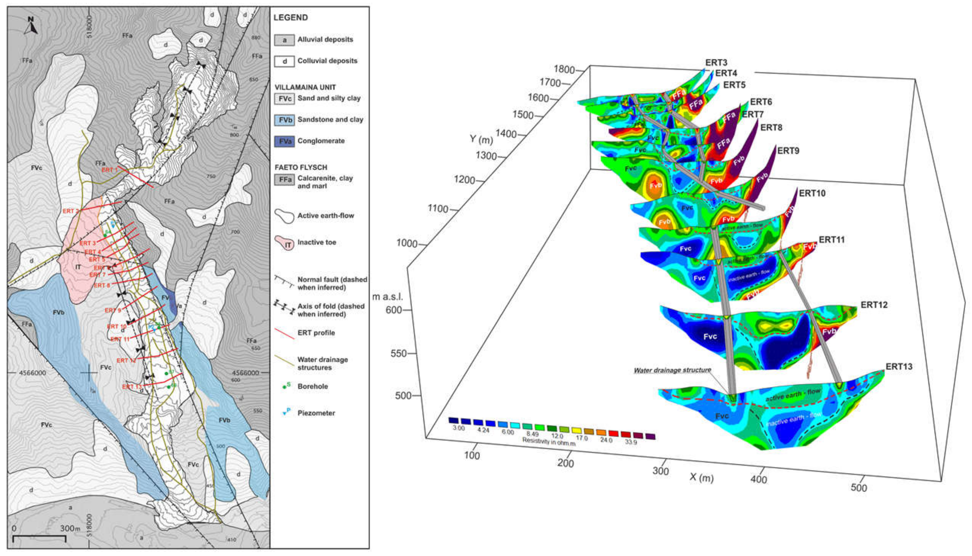
  44. Bellanova, J.; Calamita, G.; Giocoli, A.; Luongo, R.; Macchiato, M.; Perrone, A.; Uhlemann, S.; Piscitelli, S. Electrical resistivity imaging for the characterization of the Montaguto landslide (southern Italy). Eng. Geol. 2018, 243, 272–281. [Google Scholar] [CrossRef] [Green Version]
  45. Deceuster, J.; Kaufmann, O.; Van Camp, M. Automated identification of changes in electrode contact properties for long-term permanent ERT monitoring experiments. Geophysics 2013, 78, E79–E94. [Google Scholar] [CrossRef]
  46. Kim, J.H. Four dimensional inversion of dc resistivity monitoring data. In Proceedings of the Near Surface 2005-11th European Meeting of Environmental and Engineering Geophysics, Palermo, Italy, 4–7 September 2005; European Association of Geoscientists and Engineers: Houten, The Netherlands, 2005; p. A006. [Google Scholar]
  47. LaBrecque, D.J.; Yang, X. Difference inversion of ERT data: A fast inversion method for 3-D in situ monitoring. J. Environ. Eng. Geophys. 2001, 6, 83–89. [Google Scholar] [CrossRef]
  48. Daily, W.; Ramirez, A.; Labrecque, D.; Nitao, J. Electrical resistivity tomography of vadose water movement. Water Resour. Res. 1992, 28, 1429–1442. [Google Scholar] [CrossRef]
  49. Miller, C.R.; Routh, P.S.; Brosten, T.R.; McNamara, J.P. Application of Time-Lapse ERT Imaging to Watershed Characterization. Geophysics 2008, 73, G7–G17. [Google Scholar] [CrossRef] [Green Version]
  50. Kim, J.H.; Yi, M.J.; Park, S.; Kim, J.G. 4D inversion of DC monitoring data acquired over a dynamically changing earth model. J. Appl. Geophys. 2009, 68, 522–532. [Google Scholar] [CrossRef]
  51. Doetsch, J.; Linde, N.; Binley, A. Structural joint inversion of time-lapse crosshole ERT and GPR traveltime data. Geophys. Res. Lett. 2010, 37, L24404. [Google Scholar] [CrossRef]
  52. Herckenrath, D.; Fiandaca, G.; Auken, E.; Bauer-Gottwein, P. Sequential and joint hydrogeophysical inversion using a field-scale groundwater model with ERT and TDEM data. Hydrol. Earth Syst. Sci. 2013, 17, 4043–4060. [Google Scholar] [CrossRef] [Green Version]
  53. Jardani, A.; Revil, A.; Dupont, J.P. Stochastic joint inversion of hydrogeophysical data for salt tracer test monitoring and hydraulic conductivity imaging. Adv. Water Resour. 2012, 52, 62–77. [Google Scholar] [CrossRef]
  54. Camporese, M.; Cassiani, G.; Deiana, R.; Salandin, P.; Binley, A. Coupled and uncoupled hydrogeophysical inversions using ensemble Kalman filter assimilation of ERT-monitored tracer test data. Water Resour. Res. 2015, 51, 3277–3291. [Google Scholar] [CrossRef]
  55. Hayley, K.; Pidlisecky, A.; Bentley, L.R. Simultaneous time-lapse electrical resistivity inversion. J. Appl. Geophys. 2011, 75, 401–411. [Google Scholar] [CrossRef]
  56. Karaoulis, M.C.; Kim, J.H.; Tsourlos, P.I. 4D active time constrained resistivity inversion. J. Appl. Geophys. 2011, 73, 25–34. [Google Scholar] [CrossRef]
  57. Karaoulis, M.; Tsourlos, P.; Kim, J.H.; Revil, A. 4D time-lapse ERT inversion: Introducing combined time and space constraints. Near Surf. Geophys. 2014, 12, 25–34. [Google Scholar] [CrossRef] [Green Version]
  58. Wilkinson, P.B.; Uhlemann, S.; Meldrum, P.I.; Chambers, J.E.; Carriere, S.; Oxby, L.S.; Loke, M.H. Adaptive time-lapse optimized survey design for electrical resistivity tomography monitoring. Geophys. J. Int. 2015, 203, 755–766. [Google Scholar] [CrossRef] [Green Version]
  59. Nguyen, F.; Kemna, A.; Robert, T.; Hermans, T. Data-driven selection of the minimum-gradient support parameter in time-lapse focused electric imaging. Geophysics 2016, 81, A1–A5. [Google Scholar] [CrossRef]
  60. Liu, B.; Liu, Z.Y.; Li, S.C.; Fan, K.R.; Nie, L.C.; Zhang, X.X. An improved Time-Lapse resistivity tomography to monitor and estimate the impact on the groundwater system induced by tunnel excavation. Tunn. Undergr. Space Technol. 2017, 66, 107–120. [Google Scholar] [CrossRef]
  61. Lesparre, N.; Nguyen, F.; Kemna, A.; Robert, T.; Hermans, T.; Daoudi, M.; Flores-Orozco, A. A new approach for time-lapse data weighting in electrical resistivity tomography. Geophysics 2017, 82, E325–E333. [Google Scholar] [CrossRef]
  62. Tso, C.H.M.; Kuras, O.; Wilkinson, P.B.; Uhlemann, S.; Chambers, J.E.; Meldrum, P.I.; Graham, J.; Sherlock, E.F.; Binley, A. Improved characterisation and modelling of measurement errors in electrical resistivity tomography (ERT) surveys. J. Appl. Geophys. 2017, 146, 103–119. [Google Scholar] [CrossRef] [Green Version]
  63. Perri, M.T.; Barone, I.; Cassiani, G.; Deiana, R.; Binley, A. Borehole effect causing artefacts in cross-borehole electrical resistivity tomography: A hydraulic fracturing case study. Near Surf. Geophys. 2020, 18, 4. [Google Scholar] [CrossRef]
  64. Saibaba, A.K.; Miller, E.L.; Kitandis, P.K. A fast kalman filter for time-lapse electrical resistivity tomography. In Proceedings of the 2014 IEEE Geoscience and Remote Sensing Symposium, Quebec City, QC, Canada, 13–18 July 2014. [Google Scholar] [CrossRef]
  65. Oware, E.K.; Irving, J.; Hermans, T. Basis-constrained Bayesian Markov-chain Monte Carlo difference inversion for geoelectrical monitoring of hydrogeologic processes. Geophysics 2019, 84, A37–A42. [Google Scholar] [CrossRef]
  66. Delforge, D.; Watlet, A.; Kaufmann, O.; Van Camp, M.; Vanclooster, M. Time-series clustering approaches for subsurface zonation and hydrofacies detection using a real time-lapse electrical resistivity dataset. J. Appl. Geophys. 2021, 184, 104203. [Google Scholar] [CrossRef]
  67. Johnson, T.C.; Hammond, G.E.; Chen, X.Y. PFLOTRAN-E4D: A parallel open source PFLOTRAN module for simulating time-lapse electrical resistivity data. Comput. Geosci. 2017, 99, 72–80. [Google Scholar] [CrossRef] [Green Version]
  68. Rucker, C.; Gunther, T.; Wagner, F.M. pyGIMLi. An open-source library for modelling and inversion in geophysics. Comput. Geosci. 2017, 109, 106–123. [Google Scholar] [CrossRef]
  69. Blanchy, G.; Saneiyan, S.; Boyd, J.; McLachlan, P.; Binley, A. ResIPy, an intuitive open source software for complex geoelectrical inversion/modeling. Comput. Geosci. 2020, 137, 104423. [Google Scholar] [CrossRef]
  70. Liu, B.; Pang, Y.H.; Mao, D.Q.; Wang, J.; Liu, Z.Y.; Wang, N.; Liu, S.H.; Zhang, X.X. A rapid four-dimensional resistivity data inversion method using temporal segmentation. Geophys. J. Int. 2020, 221, 586–602. [Google Scholar] [CrossRef]
  71. Friedel, S.; Thielen, A.; Springman, S. Investigation of a slope endangered by rainfall-induced landslides using 3D resistivity tomography and geotechnical testing. J. Appl. Geophys. 2006, 60, 100–114. [Google Scholar] [CrossRef]
  72. Lebourg, T.; Hernandez, M.; Zerathe, S.; El Bedoui, S.; Jomard, H.; Fresia, B. Landslides triggered factors analysed by time lapse electrical survey and multidimensional statistical approach. Eng. Geol. 2010, 114, 3–4. [Google Scholar] [CrossRef]
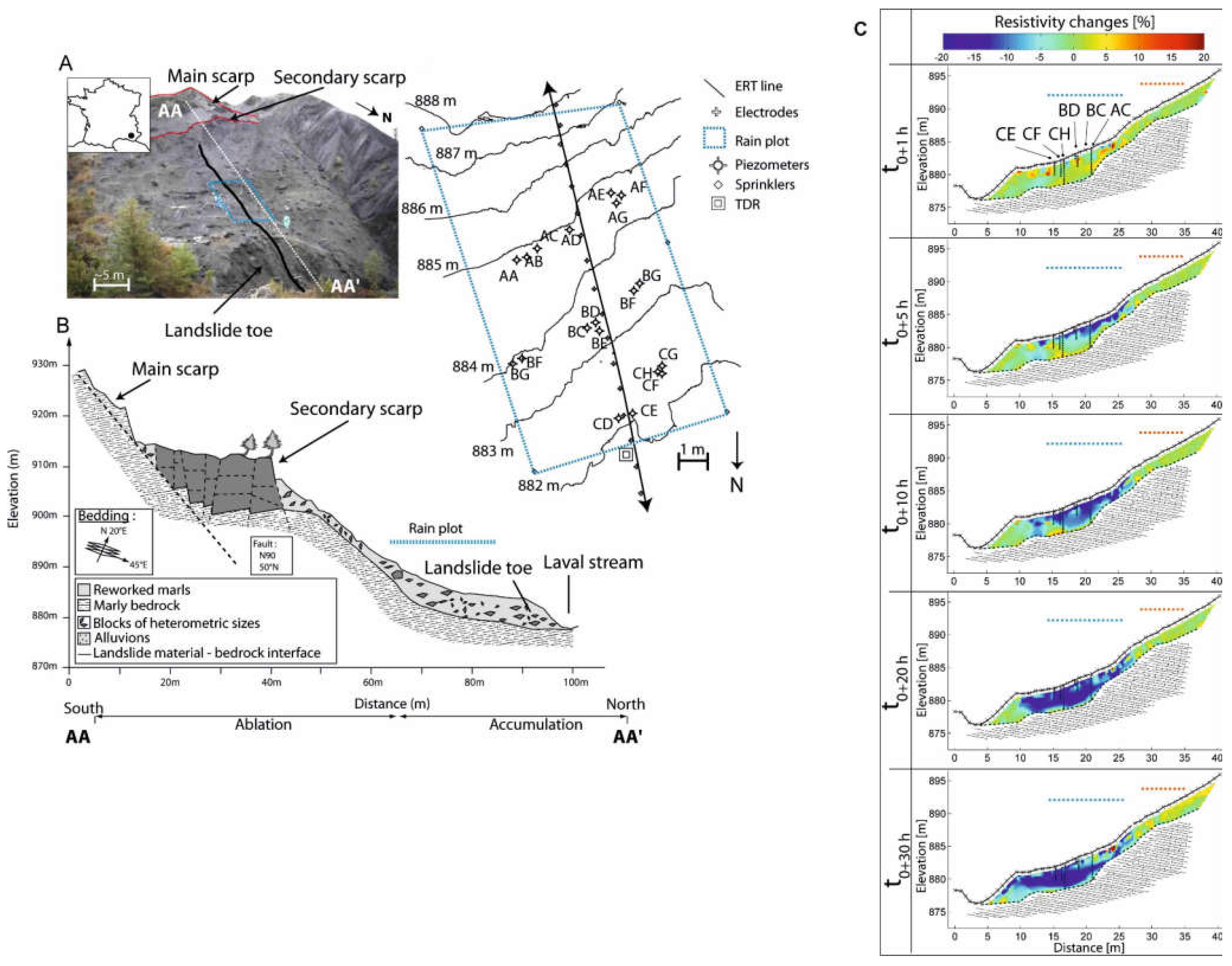
  73. Travelletti, J.; Sailhac, P.; Malet, J.P.; Grandjean, G.; Ponton, J. Hydrological response of weathered clay-shale slopes: Water infiltration monitoring with time-lapse electrical resistivity tomography. Hydrol. Processes 2012, 26, 2106–2119. [Google Scholar] [CrossRef]
  74. Lee, C.C.; Zeng, L.S.; Hsieh, C.H.; Yu, C.Y.; Hsieh, S.H. Determination of mechanisms and hydrogeological environments of Gangxianlane landslides using geoelectrical and geological data in central Taiwan. Environ. Earth Sci. 2012, 66, 1641–1651. [Google Scholar] [CrossRef]
  75. Luongo, R.; Perrone, A.; Piscitelli, S.; Lapenna, V. A Prototype System for Time-Lapse Electrical Resistivity Tomographies. Int. J. Geophysics. 2012, 2012, 176895. [Google Scholar] [CrossRef] [Green Version]
  76. Quagliarini, A.; Segalini, A.; Chelli, A.; Francese, R.; Giorgi, M.; Spaggiari, L. Joint Modelling and Monitoring on Case Pennetta and Case Costa Active Landslides System Using Electrical Resistivity Tomography and Geotechnical Data. In Advancing Culture of Living with Landslides; Mikoš, M., Casagli, N., Yin, Y., Sassa, K., Eds.; Springer: Cham, Switzerland, 2017. [Google Scholar] [CrossRef]
  77. Gunn, D.A.; Chambers, J.E.; Hobbs, P.R.N.; Ford, J.R.; Wilkinson, P.B.; Jenkins, G.O.; Merritt, A. Rapid observations to guide the design of systems for long-term monitoring of a complex landslide in the Upper Lias clays of North Yorkshire, UK. Q. J. Eng. Geol. Hydrogeol. 2013, 46, 323–336. [Google Scholar] [CrossRef]
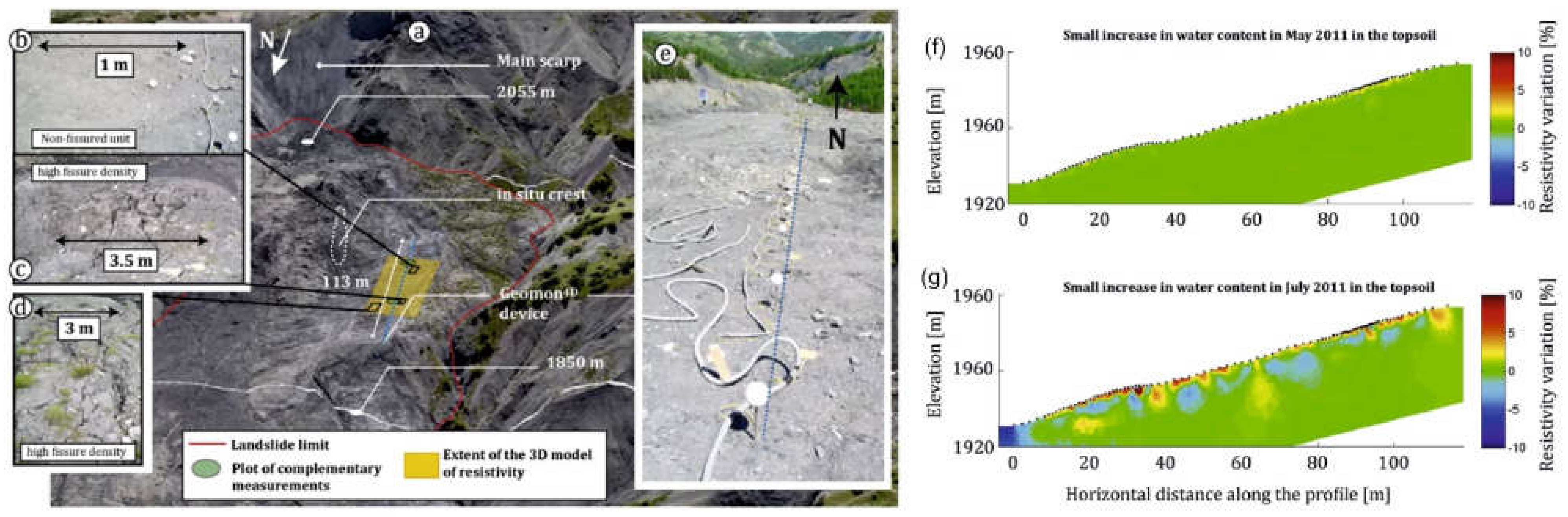
  78. Gance, J.; Malet, J.P.; Supper, R.; Sailhac, P.; Ottowitz, D.; Jochum, B. Permanent electrical resistivity measurements for monitoring water circulation in clayey landslides. J. Appl. Geophys. 2016, 126, 98–115. [Google Scholar] [CrossRef]
  79. Xu, D.; Hu, X.Y.; Shan, C.L.; Li, R.H. Landslide monitoring in southwestern China via time-lapse electrical resistivity tomography. Appl. Geophys. 2016, 13, 1–2. [Google Scholar] [CrossRef]
  80. Palis, E.; Lebourg, T.; Vidal, M.; Levy, C.; Tric, E.; Hernandez, M. Multiyear time-lapse ERT to study short- and long-term landslide hydrological dynamics. Landslides 2017, 14, 4. [Google Scholar] [CrossRef]
  81. Zieher, T.; Markart, G.; Ottowitz, D.; Romer, A.; Rutzinger, M.; Meissl, G.; Geitner, C. Water content dynamics at plot scale—Comparison of time-lapse electrical resistivity tomography monitoring and pore pressure modelling. J. Hydrol. 2017, 544, 195–209. [Google Scholar] [CrossRef]
  82. Hojat, A.; Arosio, D.; Ivanov, V.I.; Longoni, L.; Papini, M.; Scaioni, M.; Tresoldi, G.; Zanzi, L. Geoelectrical characterization and monitoring of slopes on a rainfall-triggered landslide simulator. J. Appl. Geophys. 2019, 170, 103844. [Google Scholar] [CrossRef]
  83. Ivanov, V.; Arosio, D.; Tresoldi, G.; Hojat, A.; Zanzi, L.; Papini, M.; Longoni, L. Investigation on the Role of Water for the Stability of Shallow Landslides-Insights from Experimental Tests. Water 2020, 12(4), 1203. [Google Scholar] [CrossRef] [Green Version]
  84. Boyd, J.; Chambers, J.; Wilkinson, P.; Peppa, M.; Watlet, A.; Kirkham, M.; Jones, L.; Swift, R.; Meldrum, P.; Uhlemann, S.; et al. A linked geomorphological and geophysical modelling methodology applied to an active landslide. Landslides 2021, 18, 2689–2704. [Google Scholar] [CrossRef]
  85. Mary, B.; Peruzzo, L.; Iván, V.; Facca, E.; Manoli, G.; Putti, M.; Camporese, M.; Wu, Y.; Cassiani, G. Combining Models of Root-Zone Hydrology and Geoelectrical Measurements: Recent Advances and Future Prospects. Front. Water 2021, 3, 767910. [Google Scholar] [CrossRef]
  86. Mollehuara Canales, R.; Kozlovskaya, E.; Lunkka, J.P.; Guan, H.; Banks, E.; Moisio, K. Geoelectric interpretation of petrophysical and hydrogeological parameters in reclaimed mine tailings areas. J. Appl. Geophys. 2020, 181, 104139. [Google Scholar] [CrossRef]
  87. Archie, G. The electrical resistivity log as an aid in determining some reservoir characteristics. Trans. AIME 1942, 146, 54–62. [Google Scholar] [CrossRef]
  88. Glover, P.W.J. A generalized Archie’s law for n phases. Geophysics 2010, 75, E247–E265. [Google Scholar] [CrossRef] [Green Version]
Figure 1. Yearly variations of the number of ISI articles concerning the topic “time-lapse ERT” spanning the period 2001–2020 (Source data: WoS database).
Applsci 12 01425 g001
Figure 2. (Left) Geological map of the Montaguto earth-flow (Campania region, southern Italy) with the location of direct and indirect investigations. Red lines: ERT profiles. Green line: water drainage structures. Green dot: borehole. Blue triangle: piezometers. (Right) Fence diagram showing the locations of the 2D ERT (ERT 3–ERT 13) within a 3D space (after [44]).
Applsci 12 01425 g002
Figure 3. (A) Laval landslide (ORE Draix, South French Alps) with location of the ERT line and of the equipment used for the rain experiment. (B) Cross section of the landslide. (C) Resistivity changes during the rain experiment (after [73]).
Applsci 12 01425 g003
Figure 4. The map above (a) shows the location of the investigations carried out on the Super-Sauze landslide (Southeast France). The slope is characterized by non-fissured unit (b) and areas affected by a high fissure density (c,d). The dashed blue line (e) indicates the position of the GEOMON 4D system. The images (f,g) illustrate the soil cooling effect due to the rainwater. The percentage change in soil electrical resistivity after a small rainfall event could be due to the difference between rain and initial soil temperature (after [78]).
Applsci 12 01425 g004
Figure 5. The map at the top reports the location of the survey carried out on the Vence landslide (south-eastern France), a simplified geological cross section (a) obtained along the sliding direction and the layout of the field survey carried out in the area. (b) Legend. The images below show (c) the variations of the daily median values of the three clusters of apparent resistivity measurements identified for the slope in the period 2006–2016, and (d) the accumulated rainfall index and groundwater level obtained by direct measurements in C6 and C20 for the same period (after [80]).
Applsci 12 01425 g005
Figure 6. (a) The baseline inverted image of the Hollin Hill landslide (southern Howardian Hills, UK) measured in May 2016; (b) surface resistivity in relation to a hill-shaded relief map from a UAV survey in May 2016. The six images on the right (ch) report an overview of elevation and electrode coordinate changes at Hollin Hill, as captured by terrestrial LiDAR (after [84]).
Applsci 12 01425 g006
Table 1. Simplified classification of the different approaches and methods adopted in the TL-ERT data processing and inversion. The scheme is based on the analysis of a selected list of papers published in the last ten years.
Main Classes of the Methods for the TL-ERT Data Analysis and InversionList of the Papers
Joint-inversion with other geophysical data and hydro-geophysical data.Doetsch et al., 2010
Herckenrath et al., 2013
Jardani et al., 2013
Camporese et al., 2015
Full 4D inversion, time and space active constraints, space and time regularization, algorithms based on the adaptive approaches and minimum gradients.Hailey et al., 2011
Karaoulis et al., 2011
Karaoulis et al., 2014
Wilkinson et al., 2015
Nguyen et al., 2016
Methods for minimizing the errors and the artifacts.Liu et al., 2017
Lesparre et al., 2017
Tso et al., 2017
Bievre et al., 2018
Perri et al., 2020
Clustering, Bayesian and other statistical approaches.Saibaba et al., 2014
Oware et al., 2019
Delforge et al., 2021
Open-source codes and HPC techniques.Johnson et al., 2017
Rucker et al., 2017
Blanchy et al., 2020
Liu et al., 2020
Publisher’s Note: MDPI stays neutral with regard to jurisdictional claims in published maps and institutional affiliations.

