Optically Pumped Magnetometer Measuring Fatigue-Induced Damage in Steel

Featured Application

Piezomagnetic fatigue testing of ferromagnetic specimens with highly sensitive optically pumped magnetometers as a method for early damage formation detection.

Abstract

Uniaxial fatigue testing of micro-mechanical metallic specimens can provide valuable insight into damage formation. Magnetic and piezomagnetic testing are commonly used for qualitative characterization of damage in ferromagnetic specimens. Sensitive and accurate measurements with magnetic sensors is a key part of such a characterization. This work presents an experimental setup to induce structural defects in a micro-mechanical fatigue test. Simultaneously, the resulting piezomagnetic signals are measured during the complete lifetime of the tested specimen. The key component is a highly sensitive optically pumped magnetometer (OPM) used to measure the piezomagnetic hysteresis of a small specimen whose structural defects can be analyzed on a small scale by other metallographic characterization methods as well. This setup aims to quantify the magnetic signatures of damage during the fatigue process, which could enable non-destructive mechanical testing of materials. This paper reports the initial results obtained from this novel micro-magneto-mechanical test setup for a ferritic steel specimen.

1. Introduction

Magnetic material testing methods are well-established for non-destructive testing (NDT) of materials or devices composed of steel, cast iron, or other ferromagnetic materials [1]. The fundamental principle involves an outer field $H$ applied to a ferromagnetic material to measure the response of the specimen to the exciting field $H$. This concept is utilized by some of the most frequently applied NDT techniques, such as magnetic flux leakage (MFL), magnetic Barkhausen noise (MBN), and more recently, metal magnetic memory (MMM) [2]. Using either one of these techniques as a kind of “magnetic microscope”, one can investigate the microstructure of ferromagnetic materials [3]. Additionally, these NDT techniques can routinely be applied to industrial in-line monitoring of manufacturing processes.

Alternatively, testing is possible based on the phenomenon of mechanical stresses altering the intrinsic magnetization state of ferromagnetic materials. This effect is the so-called magneto-mechanical Villari effect, which is also known as the magnetoelastic or piezomagnetic effect [4,5]. It was used to indirectly measure the fatigue state through the magnetic response of a ferromagnetic material exposed to cyclic loading [6]. In this scenario, a sensor is positioned in the specimens’ vicinity to measure the magnetic stray field originating from the specimen. Then, piezomagnetic hysteresis curves are used to identify early signs of fatigue damage in materials [7]. The shape of these hysteresis curves evolves continuously and to some extent irreversibly due to magnetic domain wall motion, their pinning at defect sites, and the generation/elimination of defects [8]. Relevant microscopic defects for such interactions include dislocations, grain boundaries, precipitates, and non-magnetic inclusions. However, stress concentrations associated with macroscopic plasticity traces and cracks also affect the magnetic stray field. Many attempts have been made to correlate the magnetic response of the material to the microstructural changes produced by fatigue, but the quantification of damage in the material remains a difficult challenge. To lay the groundwork, we combine highly sensitive quantum sensors with miniaturized specimens, which permits detailed microstructural investigation.

Previous work in this direction used specimens with rather large volumes under load ($V_{specimen}~$few cm³). This hampers a more detailed mechanistic understanding and its correlation to the magnetic response with damage because localized defect events, such as macroscopic crack initiation (typically a multiple of grain size), occur in larger volumes [9,10,11,12]. In contrast, we investigate magnetic stray fields originating from fatigue loading of mesoscale ferromagnetic specimens ($V_{specimen}~0.1$mm³). The smaller volume confines the fatigue process. Thus, damage will affect a more significant volume of the specimen and thereby be more visible in the piezomagnetic signal. Therefore, we propose the retrieval of more comprehensive magnetic information of the complete specimen volume by using optically pumped magnetometers (OPMs) [13]. The main objective is to exploit the high magnetic sensitivity of such sensors to find signs of materials’ fatigue before the formation of visible surface-residing cracks. The small volume of the mesoscale specimen produces only very faint magnetic signals that are only retrievable by high-sensitivity sensors, such as OPMs. Thus, this holds the potential to facilitate correlations between magnetic signals and localized damage events, such as plastic deformation, macroscopic crack initiation, and crack growth. The small specimen size also permits complementary characterization techniques across the whole specimen, e.g., electron backscatter diffraction or spatially resolved magnetometry [14], to reveal internal microstructural features. Furthermore, the small specimen sizes lead to comparatively high spatial resolution in computer tomography-based porosity analyses.

The technological development of OPMs has seen great progress in recent years, from their modest beginnings as large lamp pumped sensors [15], to the first miniaturized sensors in a laboratory [16] and the first commercial miniaturized sensors [17]. Based on these developments, several startup companies have started to sell OPMs. The most prominent application case of these commercial OPMs is magnetoencephalography (MEG) [18]. However, the exceptional characteristics of these sensors has led to work with either commercial or self-made sensors in fields, such as zero-field NMR spectroscopy [19], electro-chemical battery characterization [20], and materials testing [21]. The current OPM research in the field of materials testing has mainly concentrated on non-destructive measurement of metallic specimens [21]. In this work, we adopt the OPM technology for materials testing of ferromagnetic specimens under mechanical fatigue loading.

This paper is divided into three parts. First, we describe the mechanical and magnetic subsystems of the experimental apparatus. Then, we describe the relevant physical observables of the setup. Finally, we present the measurement results with this novel setup using a ferritic steel specimen.

2. Experimental Procedures

Several different types of OPMs are commercially available and they can be sorted into two main classes: zero-field OPMs and total-field OPMs. Zero-field OPMs achieve sensitivities below 50 fT/$\sqrt{\mathrm{Hz}}$ but require a very low environmental magnetic field $B$ (<50 nT) due to their limited measurement range. Total-field OPMs are less sensitive (<1 pT/$\sqrt{\mathrm{Hz}}$) but can operate in the Earths’ magnetic field. In this work, we use a commercial OPM to measure the variation of the magnetic field $B\left(t\right)$ of a ferromagnetic specimen, which is placed under a cyclic mechanical load controlled by a strain $\epsilon \left(t\right)$. 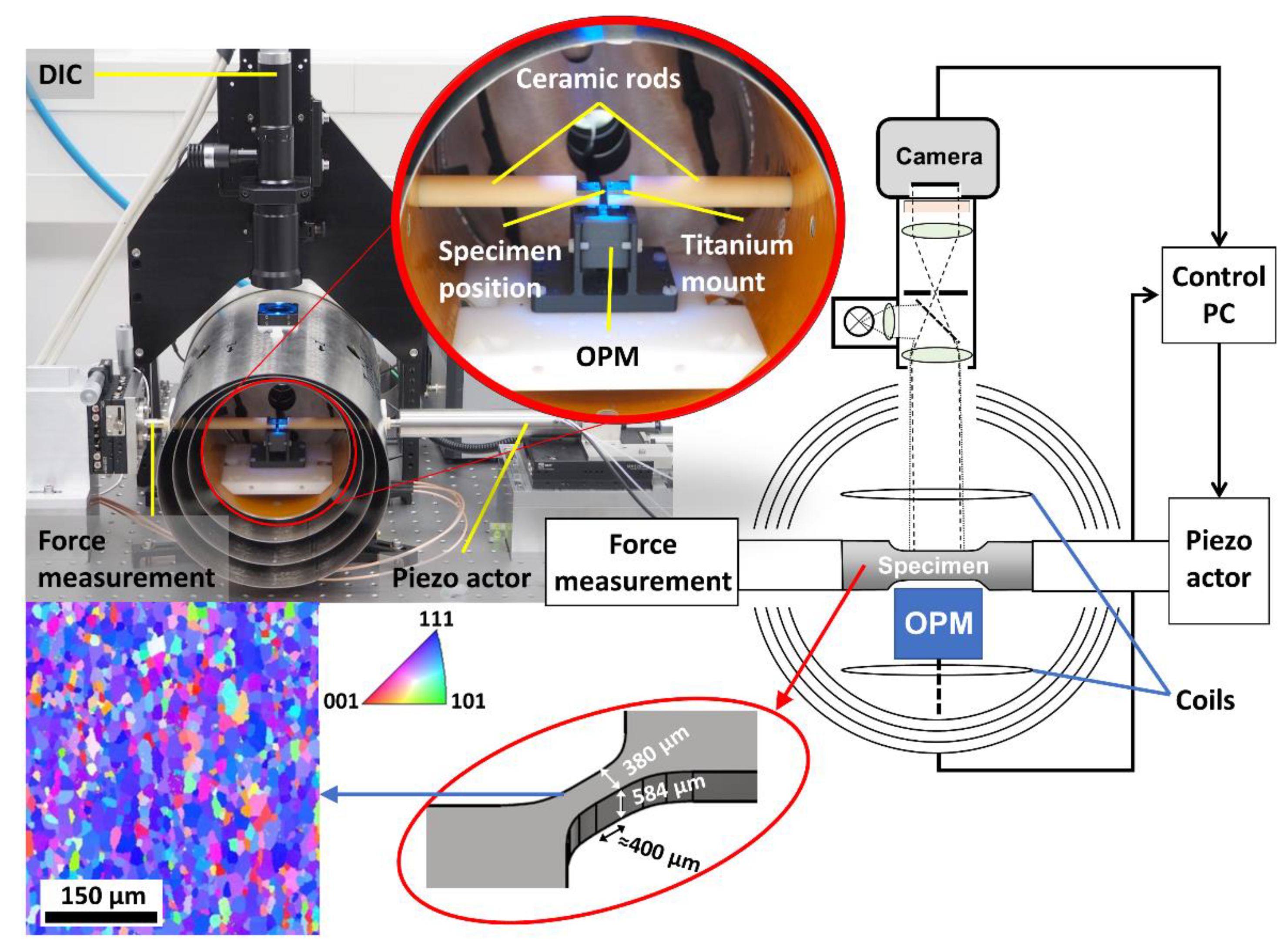The setup presented in Figure 1 uses a zero-field OPM, namely QZFM Gen2 from QuSpin (Louisville, US-CO). However, to exploit the full sensitivity of the OPM, ambient noise from various sources, such as piezoelectric sensors, actuators, or moving components close to the OPM, is suppressed to a level similar or lower than the sensitivity of the OPM. The main idea behind the setup is to mount the OPM and the mesoscopic specimen under test (SUT) in a magnetically shielded environment. The mechanical forces of the tensile testing setup are guided to the specimen by a construction employing only non-magnetic parts.

For this setup, we redesigned a micro-mechanical tensile testing device in such a way that the SUT and the OPM are mounted in proximity to each other inside a magnetic shield (Twinleaf, MS-1L, Plainsboro, US-NJ) [22]. The magnetic shield comprises four concentric cylindrical layers of mu-metal to isolate the OPM and the SUT from external electromagnetic fields. Mu-metal is a nickel-iron alloy, which features a very high permeability (${\mu }_r~ {10}^5$), which allows it to shield an environment from magnetic fields. An internal system of coils allows active compensation of residual magnetic fields to provide appropriate field strengths and homogeneity in the center of the mu-metal shield. A non-magnetic breadboard and sensor holder serve as a mount for the OPM. For uniaxial tensile testing, a piezoelectric actuator with a low stray field applies a cyclic mechanical load to the right end of the SUT. On the left, the resulting force F(t) is measured to calculate the engineering stress $\sigma \left(t\right)=F\left(t\right)/A$ using the initial cross-sectional area $A$ of the specimen.

The tensile testing machine accommodates two actuators, a linear motor (Physik Instrumente, M-238.5PL, Karlsruhe, Germany) and a piezo actuator (Physik Instrumente, P-216.90, Karlsruhe, Germany), imposing a tensile or compressive load on the SUT. Depending on the range of loading, displacements, and the necessary dynamics, either one of the loading modes can be employed. In the present work, load was applied solely with the piezo actuator. The load is conveyed to the SUT through load-carrying bars and dovetail clamps, which hold the SUT in place. The load is measured by a load cell (TE connectivity, XFTC-300-500, Schaffhausen, Switzerland), which has a dynamic range of 500 N. The load can be applied either under force-, displacement- or strain-controlled mode.

The measurement of strain on such a small specimen is a special challenge. Strain gauges are hardly applicable as they are large and produce magnetic fields through the resistance measurement of electric currents. Mechanical extensometers are too large as well and require significant pressure on the specimen surface to avoid slippage. Therefore, we used an optical real-time DIC system based on a Basler acA2040-180km camera with 2040 × 2040 pixel with a pixel pitch of 5.5 µm, allowing up to 1200 integral strain measurements per second on 2 subsets per image due to GPU evaluation [23]. To avoid magnetic perturbations from the camera electronics and LED illumination on the OPM sensor, both, the camera and lens, were mounted outside of the mu-metal shield as shown in Figure 1. To use the full resolution of 2000 pixels per line, a telecentric lens with coaxial illumination, a magnification of 1:3, and a working distance of at least 150 mm would be ideal. However, such lenses are scarce, and we used one with a magnification of 1:2 (VS-THV2-150CO/S), resulting in an object side resolution of 2.75 µm/pixel. The 2 subsets with a size of 51 × 51 pixel, i.e., the inner green squares in Figure 2a, measure integral strain. This is analogous to a mechanical extensometer placed at the beginning of the dovetails of the SUT at a distance of 469 pixels (1.3 mm). This gives the base length for integral strain measurement. The outer green squares in Figure 2a mark the search areas where path-independent correlation is possible. This allows for more robust strain-control. In combination with blue LED illumination (4W electrical power at 465 nm), a strain sampling rate of 600 Hz was achieved, which is sufficient for strain-controlled low-cycle fatigue tests (LCF) according to ASTM E606 [24]. In addition, the DIC system can be used to quantify effects, such as stress or strain concentrations, e.g., at crack tips, in full-field mode [25]. Furthermore, surface imaging facilitates the detection of surface protrusions and cracks with advanced computer vision techniques [26].

The ferritic steel specimen was extracted from cold-rolled sheets with the specimen axis pointing in the transversal direction. A strong crystallographic anisotropy is present because of this processing. The information on the alloy composition cannot be disclosed because of a confidentiality agreement. Static tensile tests on macroscopic specimen revealed a yield strength Rp__0,2 of 170 MPa. The mesoscale test specimens are fabricated with conventional wire erosion and micro wire erosion. Thus, specimen dimensions in the order of a few hundred micrometers can be obtained. At this scale, complementary characterizations by different techniques can be carried out for the whole volume of a specimen. Moreover, individual damage locations, such as early cracks, affect the load signal and the magnetic response in a pronounced manner, rendering the measurement more sensitive. In contrast to specimens with conventional macroscopic sizes, here the whole specimen volume can be monitored with the OPM without compromising the sensitivity. For full coverage of larger specimens, the specimen–sensor distance must be increased, which decreases the sensitivity of the magnetic measurement. The magnetic field variations in Figure 2 are on the level of only a few nT. This is significantly smaller than the magnetic fields produced by larger specimens [7,12]. Our aim with this approach is to fully exploit the sensitivity of OPMs to measure more details of the stray field of the specimen.

The workflow followed to operate this setup and to perform a full measurement on a specimen comprises the following steps:

(1)

Placing the specimen in the dovetail clamps of the titanium mount inside of the mu-metal shield;

(2)

Reducing environmental fields in the magnetic shield below 10 nT using the coil system shown in Figure 1;

(3)

Mechanical loading of the specimen by exerting a tension and compression force on the specimen;

(4)

Measuring a change in the magnetic field $B$ in the vicinity of the specimen using the readout of the OPM.

Apart from the tuned geometry, specimen buckling was prevented by specimen alignment. The lateral specimen holder alignment was confirmed using dedicated alignment markers in the holders while the vertical alignment was approximated by focusing on the support area of both holders.

3. Description of the Experimental Observables

The magnetic field $\overrightarrow{B}\left(t\right)$ at the magnetometers’ location is a sum of several contributions:

$$\overrightarrow{B}\left(t\right)={\mu }_0\left(\overrightarrow{H}\left(t\right)+\overrightarrow{M}\left(t\right)\right) ,$$

(1)

where $\overrightarrow{M}\left(t\right)$ is the macroscopic magnetization of the specimen and represents the observable of interest. The field $\overrightarrow{H}\left(t\right)$ is composed of the Earths’ magnetic field, magnetic fields generated by the coils of the setup, and other environmental sources.

In ferromagnetic materials without an external load, the magnetization $\overrightarrow{M}\left(t\right)$ exhibits a hysteresis due to irreversible pinning between domain walls, which are driven by the field $\overrightarrow{H}\left(t\right)$. Inhomogeneities in the crystal, such as dislocations, regions of inhomogeneous strain, and any precipitates or nonmagnetic inclusions within grains, contribute to the hysteresis behavior as well [8]. In piezomagnetic testing, the magnetization is changed by the additional application of a mechanical stress $\sigma$ via magnetoelastic coupling. This is the so-called Villari effect. The applied stress acts as a strong field $H$, shifting domain walls and causing similar pinning effects with dislocations [27]. Thus, the magnetization of a ferromagnetic specimen depends on the evolution of the mechanical parameters applied to the specimen as [28]:

$$\overrightarrow{M}\left(t\right)={{\displaystyle \int }}_V\overrightarrow{m}\left(\overrightarrow{x}, \sigma \left(\overrightarrow{x}, t\right),t\right)d\overrightarrow{x},$$

(2)

where $\sigma$ is the mechanical stress applied to the specimen and $\overrightarrow{m}$ the magnetic moment at location $\overrightarrow{x}$. If the applied field $\overrightarrow{H}\left(t\right)$ is constant, as can be achieved in this piezomagnetic testing setup, changes in $\overrightarrow{B}\left(t\right)$ are proportional to the magnetization $\overrightarrow{M}\left(t\right)$.

The present experimental setup aims to find early indicators of fatigue damage in materials. The setup produces both mechanical (F$-\epsilon$) hysteresis curves and piezomagnetic ($B-\epsilon$) hysteresis curves. An important aspect of such hysteresis curves is the area delimited by the curve [5]. By measuring the area delimited by these curves, we expect to be sensitive to the energy involved in the deformation process of the specimen. For a non-oriented ferromagnetic material with homogeneous magnetostriction, the magnetoelastic energy, $E_{\sigma }^e$, has the following proportionality:

$$E_{\sigma }^e\propto -\frac{2}{3}\lambda \sigma ,$$

(3)

where λ is the effective magnetostriction constant of the material and $\sigma =F/A$ is the uniaxial mechanical stress applied by a force $F$ to a specimen with cross-section $A$ [27]. Both the outer magnetic field $H$ and mechanical stress $\sigma$ cause domain wall motion in ferromagnetic materials. Specific points of interest on the piezomagnetic hysteresis are the so-called “Villari reversals” near the transitions from tensile to compressive stress. For uniaxial tensile stress, magnetic domains with moments parallel to the stress grow at the cost of those with perpendicular directions, whereas compressive stress increases domains with moments perpendicular to the stress. Therefore, significant amounts of domain wall motion and defect interaction can be expected at these points.

4. Test Results and Discussion

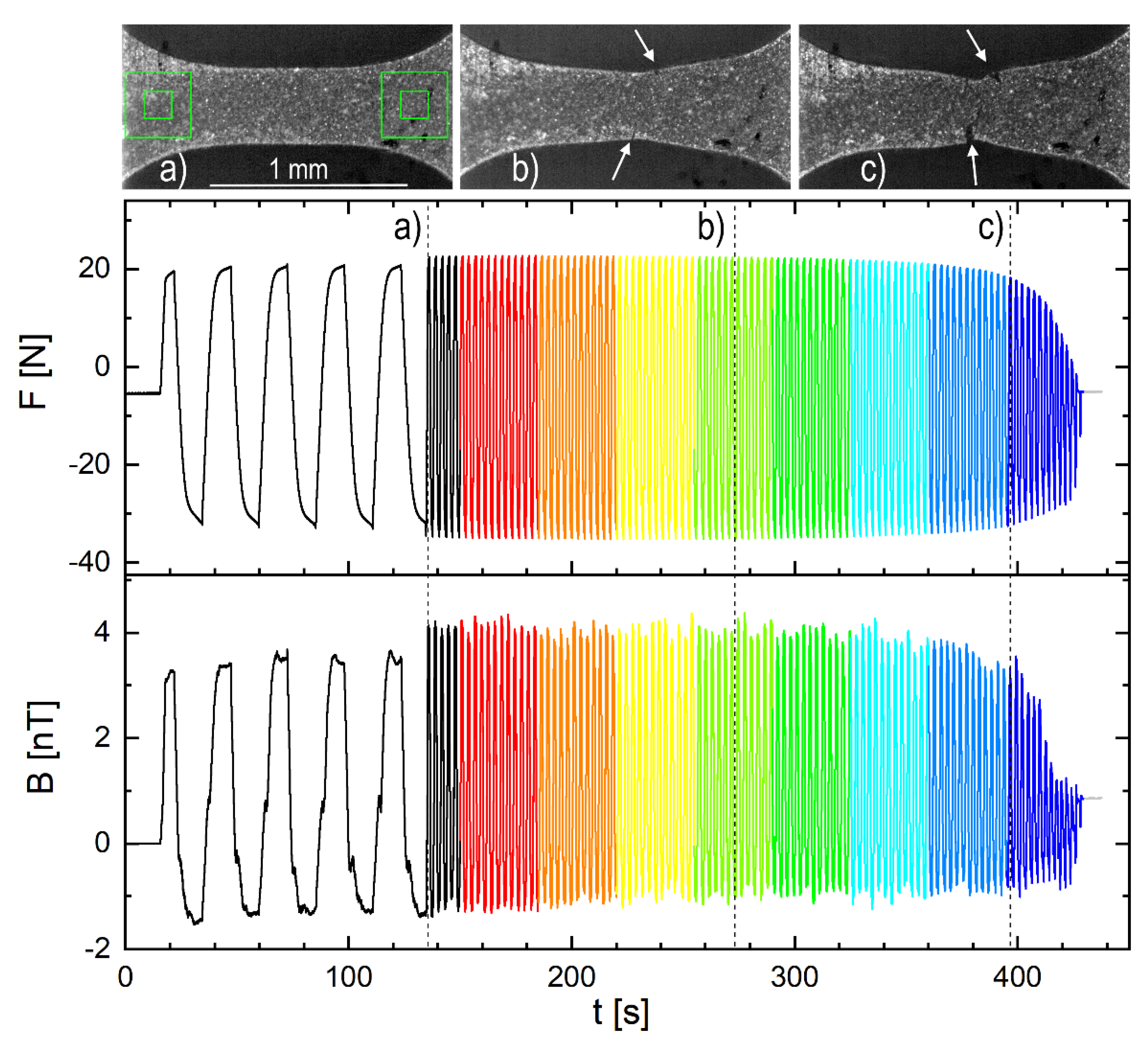
Figure 2 shows piezomagnetic signals together with optical DIC images from a strain-controlled low-cycle fatigue (LCF) experiment. A specimen made of ferritic steel was chosen since it produces a large magnetic signal. It has a cross-section of 0.22 mm² and the straight part of the target gauge is 400 µm long (detailed in Figure 1). The strain amplitude of ±1.5% results in a lifetime of 108 cycles. The magnetic time series in Figure 2 looks less smooth and less stable than the force time series. First, controlling the magnetic environment at an nT level becomes a challenge even with a multilayer mu-metal shield. Then, the magnetic time series contains richer information, which becomes clearer when represented as hysteresis curves in Figure 3. However, the general trend, where the signal becomes smaller as the specimen reaches failure, is clearly visible on both traces. The magnetic time series shows a significant shift around the zero crossing. This could be due to the fact that the specimen was not demagnetized before this measurement.

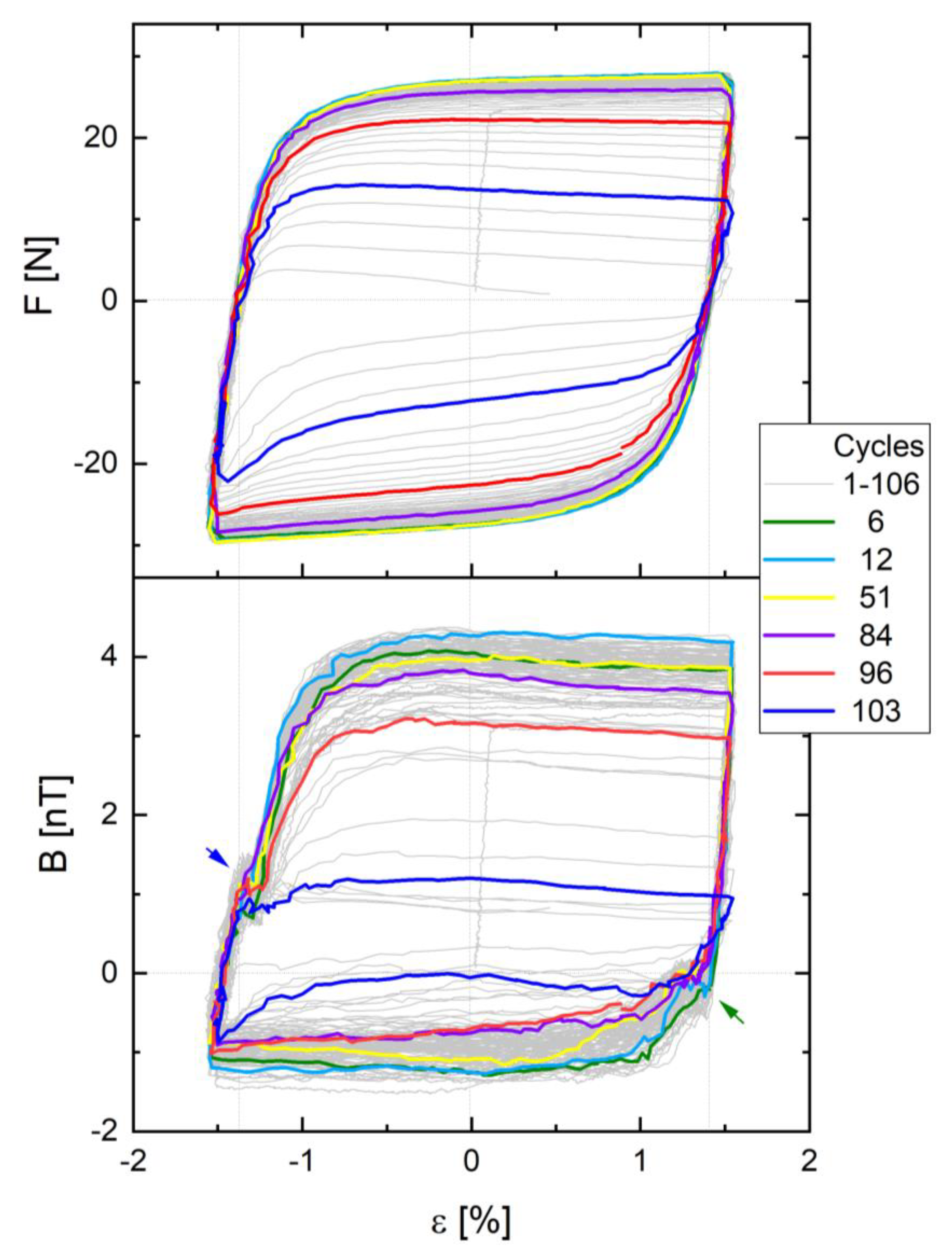
Figure 3 shows the hysteresis curves corresponding to the data displayed in Figure 2. These curves represent the main observables of the setup, which can be measured with our apparatus. The complete set of curves over cycles 1 to 106 is drawn in light grey and some of the curves are highlighted with colors. Cycle 6 corresponds to Figure 2a, cycle 51 to macroscopic crack initiation (Figure 2b), and cycle 96 to rapid crack growth (Figure 2c). At cycle 84, the force amplitude dropped by 5%, which is a common indicator for end-of-life. Cycle 103 is the last cycle before complete rupture. Until macroscopic crack initiation at cycle 51, the damage is assumed to be somewhat homogenous throughout the gauge section of the SUT. However, significant stress and defect concentrations occur near the crack tips during crack growth at cycle 96.

The shape and the area of the hysteresis curves evolve as the SUT undergoes fatigue. The mechanical (F$-\epsilon$) hysteresis is used more widely than the piezomagnetic ($B-\epsilon$) hysteresis. The mechanical hysteresis curves overlap until cycle 51 and remain fairly constant in size and shape until cycle 84, where rapid crack growth starts as shown in Figure 2c. This drop is presumably due to the fatigue-induced reduction of the specimens’ cross-section. The area delimited by the mechanical hysteresis curve is related to the energy for plastic deformation of the specimen. The rest of the energy is dissipated in the form of heat [29].

In contrast to the mechanical hysteresis, where almost all cycles have overlapping curves up to macroscopic crack initiation, the piezomagnetic curves clearly change their shape and size upon cycling. They reach the maximum area at cycle 12 and shrink continuously afterwards. In addition, the piezomagnetic curves exhibit distinct “dent” features near the zero-transitions of the force F (marked by the arrows in Figure 3). These “dent” features may be referred to as “Villari reversals”, where the subsequent slight decrease in the magnetic field is potentially associated with a change in the sign of the magnetostrictive constant. Under tensile stresses, domains magnetized parallel to the tensile direction grow, whereas compressive stress favors the growth of domains with perpendicular magnetization directions [4]. The positions of the Villari reversals contain information about the materials’ history and the irreversible interactions between domain walls and defects in the material. Therefore, monitoring the behavior of the Villari reversals is of particular interest as a potentially good indicator for early detection of defects generated or evolving with fatigue. The aim for the detection of early defect formation is to find a magnetic signature before macroscopic crack initiation at cycle 51.

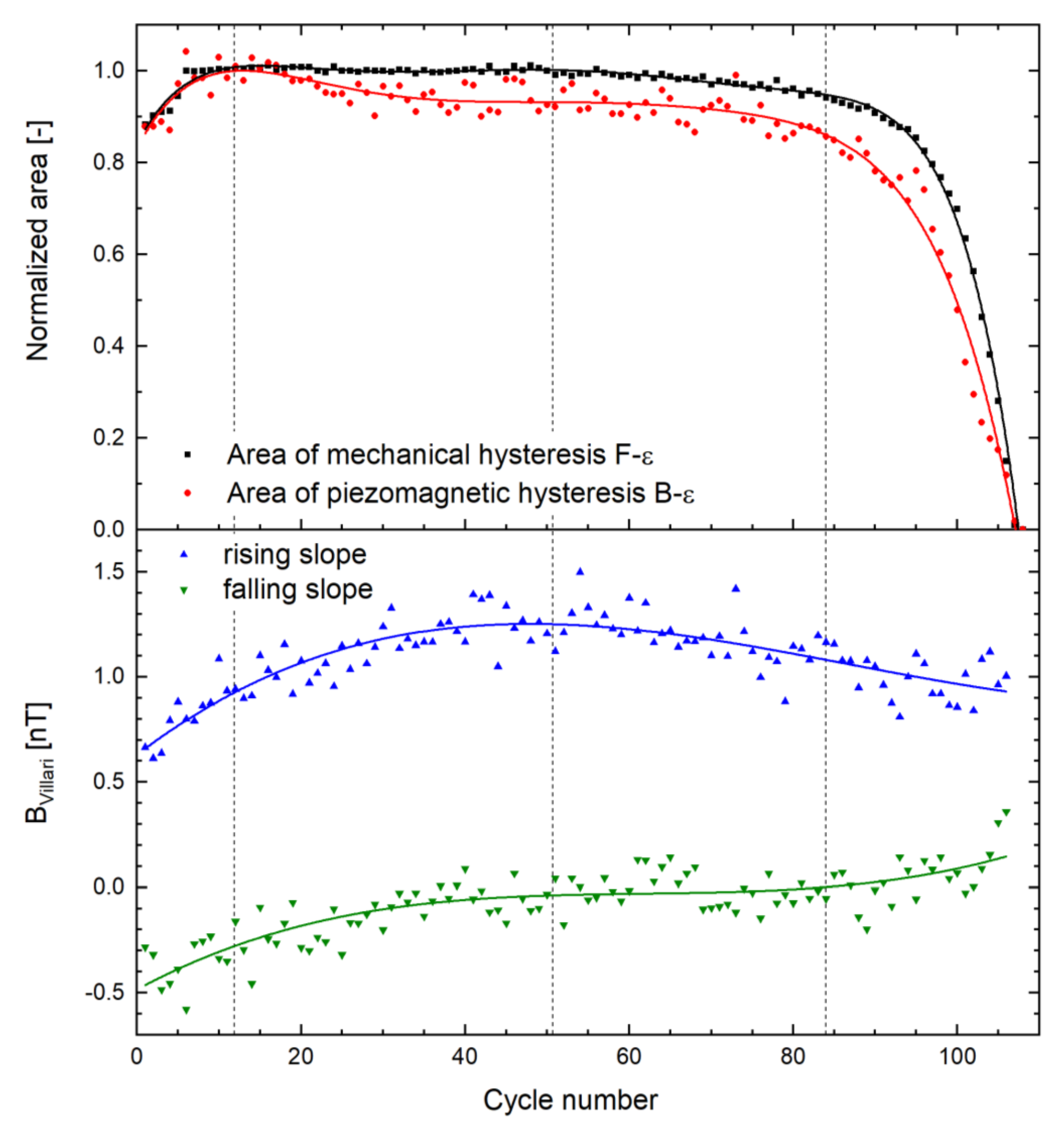
Figure 4 shows features that can be extracted from the data generated with this setup. We present the temporal evolution of 2 potential signatures derived from the hysteresis curves in Figure 3. On the top, the areas of the mechanical and the piezomagnetic curves are drawn. The dots and squares mark the values measured by integration of each cycle and the lines are fit with a seventh degree polynomial. As strain is a unitless quantity, the units of the areas are those of force F in case of the mechanical and of magnetic field B in case of the piezomagnetic curve. Therefore, they are normalized to their common maximum at cycle 12 (first dashed line) with values 1.46 N in the mechanical and 0.14 nT in the magnetic curve. Both curves rise in parallel in the first six cycles, which might be caused by some initial hardening. Alternatively, this might be due to the manual change in the frequency after cycle 5 since this comes along with an increase in the force amplitude. The area of the mechanical curve remains almost constant until cycle 84 (dashed line on the right), whereas the piezomagnetic curve drops between cycles 12 and 40. Afterwards, it exhibits a plateau and drops after cycle 84, i.e., in the range of rapid crack growth. Thus, it exhibits a much earlier reaction to fatigue-induced damage than the area of the mechanical curve.

The second potential signature of early damage detection is the magnetic field strength $B_{Villari}$ of the Villari reversals drawn on the bottom of Figure 4. The blue triangles pointing upwards are those on the rising slope (blue arrow on the left of the $B-\epsilon$ curves in Figure 3). The green triangles pointing downwards represent the corresponding reversals from the falling slopes (i.e., the compression half cycles) at the green arrow in Figure 3 (tail-reversal). Up to macroscopic crack initiation near cycle 51 (dashed line in the center), the value of $B_{Villari}$ increases for both slopes, potentially due to an increase in the defect density. Remarkably, they feature a different behavior after macroscopic crack initiation. The values from the rising slope exhibit a maximum whereas those from the falling slope increase throughout the experiment but manifest an inflection point at the macroscopic crack initiation. Thus, Villari reversals could be promising candidates for damage indicators before macroscopic crack initiation.

5. Conclusions and Outlook

This paper presents the first results from a novel experimental setup combining the generation of fatigue damage in a mesoscale specimen and retrieval of its piezomagnetic response through sensitive optically pumped magnetometers. The main advantage of this setup is the monitoring of the mechanical and especially the piezomagnetic signals with high precision and low environmental perturbations throughout the whole lifetime of the specimen under test.

The prerequisite to measuring small specimens is high-sensitivity quantum magnetometers. For a ferritic steel specimen with a cross-section of 0.22 mm² and a gauge length of 400 µm, the resulting magnetic field amplitude under plastic deformation was in the range of 5 nT. For a robust extraction of features, such as the magnetic field of the Villari reversals, environmental magnetic noise should be on the level of 1 pT. This was achieved by using a zero-field OPM in combination with a magnetic shield and a tailored non-magnetic loading unit. The stiffness of the loading unit permits testing of high-strength steels under compressive and tensile loads.

The reduced specimen volume could enable a better correlation between magnetic signals and localized damage events, such as plasticity or cracking, using complementary characterization techniques. For example, full-field DIC might be used for quantitative measurement of macroscopic crack initiation and electron backscatter diffraction can reveal internal microstructural features across the whole specimen. As the grain size of certain materials is on the order of a few hundred micrometers, investigations of individual grain boundaries become possible using the miniaturized specimen. Prospectively, even sub-surface damage, such as crack initiation at non-magnetic inclusions causing the so-called fisheye in high-strength steels, might become measurable in situ [30].

We compared the mechanical and piezomagnetic hysteresis over the entire lifetime of a ferritic steel specimen. The piezomagnetic curves showed more features than the mechanical curves. Therefore, we suggested two potential damage indicators, i.e., the area of the piezomagnetic hysteresis, such as in [5], and the magnetic field of the Villari reversals. Both responded earlier than the area of the mechanical hysteresis. In particular, the Villari reversals showed a significant increase before macroscopic crack initiation. Therefore, both might be used as early damage indicators. However, these indicators must be verified by complementary characterization and modeling [6,27,31]. On the other hand, these models also require validation, for which the setup proposed here opens new opportunities. Thereby, a broadened mechanistic understanding could be derived.